In this paper, we present an effective algorithm for solving the Poisson–Gaussian total variation model. The existence and uniqueness of solution for the mixed Poisson–Gaussian model are proved. Due to the strict convexity of the model, the split-Bregman method is employed to solve the minimization problem. Experimental results show the effectiveness of the proposed method for mixed Poisson–Gaussion noise removal. Comparison with other existing and well-known methods is provided as well.
Image acquisition is an ubiquitous technology, found for example in photography, medical imagery, astronomy, etc. Nevertheless, in almost all situations, the image-capturing devices are imperfect: some unwanted noise is added to the signal. Therefore, the obtained images are post-processed by numerical algorithms before being delivered to the users; those algorithms have to solve the image restoration problem.
In the image restoration problem, an original image u is corrupted by some random noise η, resulting in a noisy image f. Our task is to reconstruct u, knowing both f and the distribution of η. Of course, there is in general no way to find the exact image u; image restoration algorithms rather yield a good approximation of u, usually noted . To do so, they exploit a priori knowledge on the image u.
Various distributions have been considered for the noise, e.g. Gaussian (Rudin et al., 1992; Pham and Kopylov, 2015), Poisson (Chan and Shen, 2005; Le et al., 2007), Cauchy (Sciacchitano et al., 2015), as well as some mixed noise models, e.g. mixed Gaussian-Impulse noise (Yan, 2013), mixed Gaussian–Salt and Pepper noise (Liu et al., 2017), mixed Poisson–Gaussian (Calatroni et al., 2017; Pham et al., 2018; Tran et al., 2019).
A growing interest in Poisson–Gaussian probabilistic models has recently arisen (Chouzenoux et al., 2015). The mixture of Poisson and Gaussian noise occurs in several practical setups (e.g. microscopy, astronomy), where the sensors used to capture images have two sources of noise: a signal-dependent source which comes from the way light intensity is measured; and a signal-independent source which is simply thermal and electronic noise. Gaussian noise is just additive, so it cannot properly approximate the Poisson–Gaussian distributions observed in practice, which are strongly signal-dependent.
In general, the mixed Poisson–Gaussian noise model can be expressed as follows: where f is observed image, u is the unknown image, means that the image u is corrupted by Poisson noise, and is a Gaussian noise with zero mean and variance σ.
Recently, several approaches have been devoted to the mixed Poisson–Gaussian noise model (Foi et al., 2008; Jezierska et al., 2011; Lanza et al., 2014; Le Montagner et al., 2014). Many algorithms for denoising images corrupted by mixed Poisson–Gaussian noise have been investigated using approximations based on variance stabilization transforms (Zhang et al., 2007; Makitalo and Foi, 2013) or PURE-LET based approaches (Luisier et al., 2011; Li et al., 2018). Variational models based on the Bayesian framework have been also proposed for removing and denoising and deconvolution of mixed Poisson–Gaussian noise (Calatroni et al., 2017). This framework is perhaps a popular approach to mixed Poisson–Gaussian noise model. Authors in De Los Reyes and Schönlieb (2013) proposed a nonsmooth PDE-constrained optimization approach for the determination of the correct noise model in total variation image denoising. Authors in Lanza et al. (2014) focused on the maximum a posteriori approach to derive a variational formulation composed of the total variation (TV) regularization term and two fidelities. A weighted squared norm noise approximation was proposed for mixed Poisson–Gaussian noise in Li et al. (2015), or an efficient primal-dual algorithm was also proposed in Chouzenoux et al. (2015) by investigating the properties of the Poisson–Gaussian negative log-likelihood as a convex Lipschitz differentiable function. Recently, authors in Marnissi et al. (2016) proposed a variational Bayesian method for Poisson–Gaussian noise, using an exact Poisson–Gaussian likelihood. Similarily, authors in Calatroni et al. (2017) proposed a variational approach which includes an infimal convolution combination of standard data delities classically associated to one single-noise distribution, and a TV regularization as regularizing energy. Generally, image restoration by variational models based on TV can be a good solution to the mixed Poisson–Gaussian noise removal with the following formula (Calatroni et al., 2017; Pham et al., 2019): where f is the observed image, is a bounded domain, and is the set of positive functions from Ω to ; finally, are positive regularization parameters (see Chan and Shen, 2005, for details on this method).
However, in some cases, intermediate solutions of (2) obtained during the execution of algorithms may contain pixels with negative values. To avoid this problem, authors in Pham et al. (2018) proposed a modified scheme of gradient descent (MSGD) that guarantee positive values for each pixel in the image domain.
In this work, we focus on the model (2) and consider the following model: where f is the observed image, and are positive regularization parameters, is closed and convex, with being the space of functions with bounded variation; and finally is a continuous function in .
The function is used to control the intensity of the diffusion, which is an edge indicator for spatially adaptive image restoration (Barcelos and Chen, 2000). Typically, the function is chosen as follows: where l is a threshold value and , in which ∗ denotes the convolution with , i.e. the Gaussian filter with standard deviation σ.
The main contributions of this paper are the following. We give an elementary proof of the existence and uniqueness of model (3). Moreover, we check that the functional is convex, which enables us to use larger time-step parameters during gradient descent when solving (3). We introduce the influence function , which acts as an edge-detection function, to get the model (3) in order to improve the ability of edge preservation and to control the speed of smoothing. In addition, we propose a new method to solve (3) that perceptibly improves the quality of the denoised images. By changing the time-step parameter, users can either get faster denoising with comparable results to previous methods, or better quality denoising with comparable running times. Our method is a technical improvement over the split-Bregman algorithm. We report experimental results for the aforementioned method, for various parameters in the noise distribution. The quality of denoising is measured with the SSIM and PSNR metrics. If we tune the time-step parameter to get similar quality result as the original split-Bregman method, we get faster running times.
The rest of the paper is organized as follows. In Section 2, we describe the Poisson–Gaussian model and introduce the notation used in this work. In Section 3, we prove the existence and uniqueness of the solution. In Section 4, using the split-Bregman algorithm, we present the proposed optimization framework. Next, in Section 5, we show some numerical results of our proposed method and we compare them with the results obtained with other existing methods. Finally, some conclusions are drawn in Section 6.
Preliminaries
We recall the principle behind equation (2). Note that the contents of this section are not a rigorous proof; we simply provide a bit of context around the equation, why it was considered in the first place, and one possible reason for its practical efficiency. We also state our assumptions on both the initial image and the noise along the way.
Our goal is to recover the original image u, knowing the noisy image f. Our strategy is to find the image u which maximizes the conditional probability . Bayes’s rule gives: The probability density function of the observed image f corrupted by Gaussian noise (respectively, by Poisson noise ) is: where σ is the variance of the Gaussian noise. As we explained in the introduction, the two sources of noise are independent of each other, so the distribution of the mixed noise may be expressed as: We assume that the values of the pixels in the original image are independent, and that the noise is also independent on each pixel. (However, we do not assume that the noise and the original image are independent of each other.) Suppose that f has size , and let denote the domain of f. For i in I, we write the pixel of f at position i (and similarly the pixel of u at position i). Then, with . Maximizing is equivalent to minimizing , so let us compute the quantity : for some constant . In the above equation, u varies but f is constant. Since our goal is to minimize the whole expression, we can ignore the term altogether.
Now we assume that follows a Gibbs prior (Le et al., 2007): where z is a normalization factor. We need to make a couple of comments here. First, u is not a function , but rather a discrete array of pixels; thus the integral in that expression is going to be translated to a sum, while will be translated as a linear approximation. Second, this assumption appears to contradict the previous one, that the pixels of the original image are independent of one another. However, the assumption on is local: each pixel depends (weakly) on the neighbouring pixels only, so we do not lose much by assuming independence. This turns out to yield good results in practice (Chan and Shen, 2005).
We now have all the ingredients to maximize . By equation (4), this amounts to minimize the expression , so we can plug in equations (5) and (6) to get: and we can view this expression as a discrete approximation of the functional defined as: with and . (We multiplied by z, which is positive and constant, so the minimum is the same.) Intuitively, the last two terms are data fidelity terms, which ensure that the restored image u is not “too far” from the original image u (taking the distribution of the noise into account). By contrast, is a smoothness term, which guarantees that the reconstructed image is not too irregular (this is where our a priori knowledge on the original picture lies). The parameters and will have to be determined experimentally later on.
In the following sections, we introduce some theoretical results about the existence and uniqueness result for solution of (3).
Existence and Unicity of the Solution
Motivated by Aubert and Aujol (2008), Dong and Zeng (2013), we have the following existence and uniqueness results for the optimization problem (3). We prove that (3) has an unique solution in two steps: first, we show that is a convex functional; then, we show that has a lower bound. These two facts together imply the existence and uniqueness of the minimizer of .
The functional, where E is defined in (3), is strictly convex.
Let us set: . The first and the second order derivative of h are: and Since f is a positive, and , we have: , i.e. is strictly convex. Moreover, the TV regularization is convex, thence is also strictly convex. □
Let, then the problem (3) has an exactly one solutionand satisfying:
Let us denote that , and
Fixing and denoting the data fidelity term with h on , where
Easily, we have that the first order derivative of g satisfies:
The function g decreases if and increases if . Therefore, for every , we have
Hence, if , we have
Furthermore, from Kornprobst et al. (1999), we have: . Hence, . In the same way, we have: , where . Thence, we can assume , the sequence is bounded in .
Since is a minimizing sequence, we know that is bounded. Hence, also the regularization term is bounded and is bounded in .
There exists such that up to a subsequence, we have that converges weakly to and converges strongly to . We have is closed and convex. Using , the lower semicontinuity of the total variation and Fatou’s lemma, we get that is a minimizer of the problem (3). □
Numerical Method
Discretization Scheme
Our scheme allows to perform both deblurring and denoising simultaneously. To do so, we need to compute: where K is a blurring operator (convex), f is the observed image, is the set of positive functions defined over Ω with bounded total variation, and are positive regularization parameters. This functional is still strictly convex, because K is assumed to be convex.
The images we are handling are discrete, i.e. matrices of pixel values rather than functions from . Therefore we have to choose a discretization scheme for numerical computations. If u is a image, we write for the pixel at coordinates in u. We define the following quantities: where ε is a small positive number, added to avoid divisions by 0 in the implementation of the algorithms. Finding a minimum for the problem (2) can be achieved via the steepest gradient descent method The operator divergence is defined by where Thus, for a small parameter , a solution of the minimization problem (2) may be computed by When the time-step parameter becomes small, the convergence speed becomes so slow that larger images are proceeded with poor efficiency. There are many methods (Chambolle, 2004; Micchelli et al., 2011; Boyd et al., 2010) which can be used for the minimization problem in (2). In this paper, we extend the split-Bregman algorithm (Goldstein and Osher, 2009) to solve the minimization problem.
Proposed Algorithm
First, let us first review the split-Bregman algorithm (Goldstein and Osher, 2009). Suppose that we have a scalar γ and two convex functionals and ; and that we need to solve the following constrained optimization problem:
We convert (10) into an unconstrained problem: where ρ is a penalty parameter (a positive constant) and b is a variable related to the split-Bregman iteration algorithm (to be explicited later). The solution to problem (11) can be approximated by the split-Bregman Algorithm (Goldstein and Osher, 2009): Now we return to the problem (9). We define We set ; then, based on equation (11), the split-Bregman problem for (9) is defined as: where the parameters , and γ are positive, , and .
The split-Bregman method for solving (12) is described as follows:
There are three subproblems to solve: u, ν and d.
Subproblem 1. The u subproblem is a quadratic optimization problem, whose optimality condition reads: under considering periodic boundary conditions. Note that left-hand-side matrix in (13) includes a Laplacian matrix () and is strictly diagonally dominant. Following Wang et al. (2008), equation (13) can be solved efficiently with one fast Fourier transform (FFT) operation and one inverse FFT operation as: where and are the forward and inverse Fourier transform operators.
Subproblem 2. The optimality condition for the ν subproblem is given by This equation canbe rewritten as: The positive solution is given by where
Subproblem 3. The solution of the d subproblem can readily be obtained by applying the soft thresholding operator (see Micchelli et al., 2011). We can use shrinkage operators to compute the optimal values of and separately: The problem (16) is solved as:
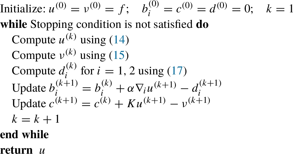
The algorithm. The complete method is summarized in Algorithm 1. We need a stopping criterion for the iteration; we end the loop if the maximum number of allowed outer iterations N has been carried out (to guarantee an upper bound on running time) or the following condition is satisfied for some prescribed tolerance ς: where ς is a small positive parameter. For our experiments, we set tolerance and .
Adaptive split-Bregman algorithm for solving the model (9).
Numerical Simulations
Implementation Issues
In this section, we show some numerical reconstructions obtained applying our proposed method for mixed Poisson–Gaussian noise. We compare our reconstructions with other images obtained other well known methods, such as TV- (Chambolle et al., 2010), the Modified scheme for Mixed Poisson–Gaussian model (MS-MPG) (Pham et al., 2018) and the Bregman method (Goldstein and Osher, 2009). All of the compared methods perform image denoising with their optimal parameters. For a fair comparison, the regularization parameters of both MS-MPG and our proposed are the same: , . We set , . The parameter σ in is set to 1. The threshold value l in the function and the parameters γ are chosen to keep the poise between noise removal and detail preservation capabilities.
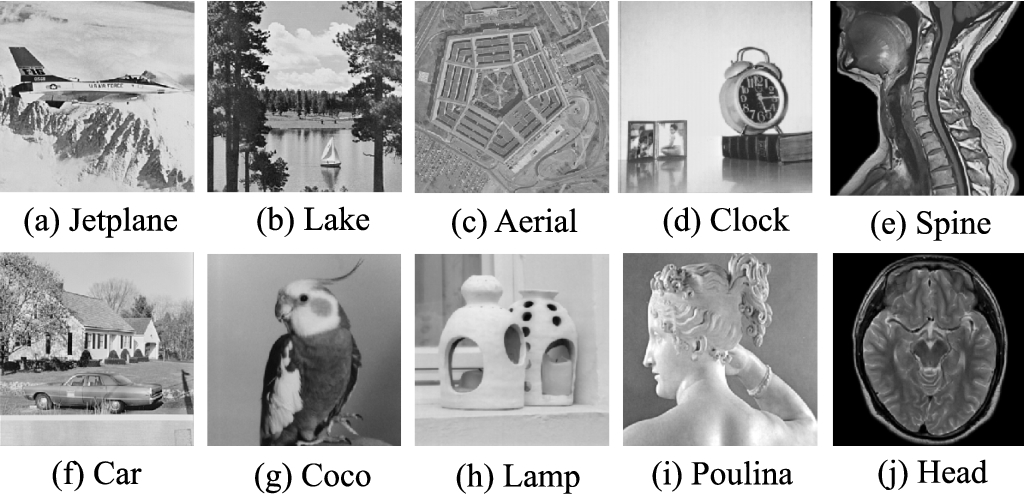
The test images1 are 8-bit gray scale standard images of size shown in Fig. 1.
Original images.
All the experiments were run on a machine with Core i7-CPU 2 GHz, SDRAM 4 GB-DDR III 2 Ghz, Windows 10 (64 bit), and implemented in MATLAB. To compare the efficiency of algorithms, we use the Peak Signal-to-Noise Ratio (PSNR) and the Structure Similarity Index (SSIM) (Wang and Bovik, 2006).
The first metric, PSNR (db), is defined by where are, respectively, the original image and the reconstructed (or noisy) image, is the maximum intensity of the original image, M and N are the number of image pixels in rows and columns.
The second metric, SSIM, is defined by where , are the means of u, , respectively; , their standard deviations; , the covariance of two images u and ; ; ; L is the dynamic range of the pixel values (255 for 8-bit grayscale images); and finally , are small constants.
Numerical Results and Discussion
Image Denoising
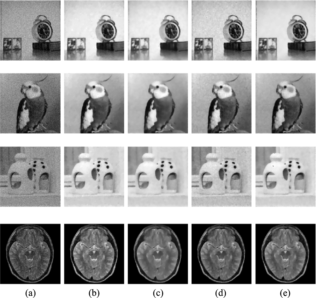
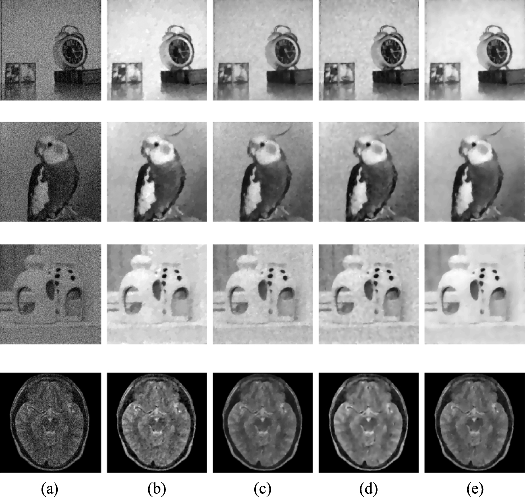
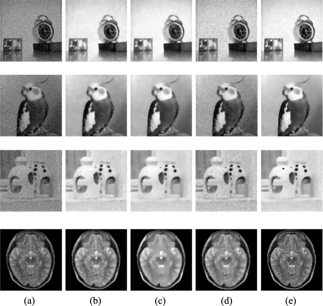
Our method can perform image deblurring and denoising simultaneously. In this section, we perform only image denoising. Noisy observations are generated by Poisson noise with some peak and by Gaussian noise with standard deviation to the test images. In Figs. 2, 4 and 5, we give the results for denoising the corrupted images for different noise levels and .
Recovered results for the test images. (a) Noisy image with , , (b) TV , (c) Bregman, (d) MS-MPG, (e) Our proposed.
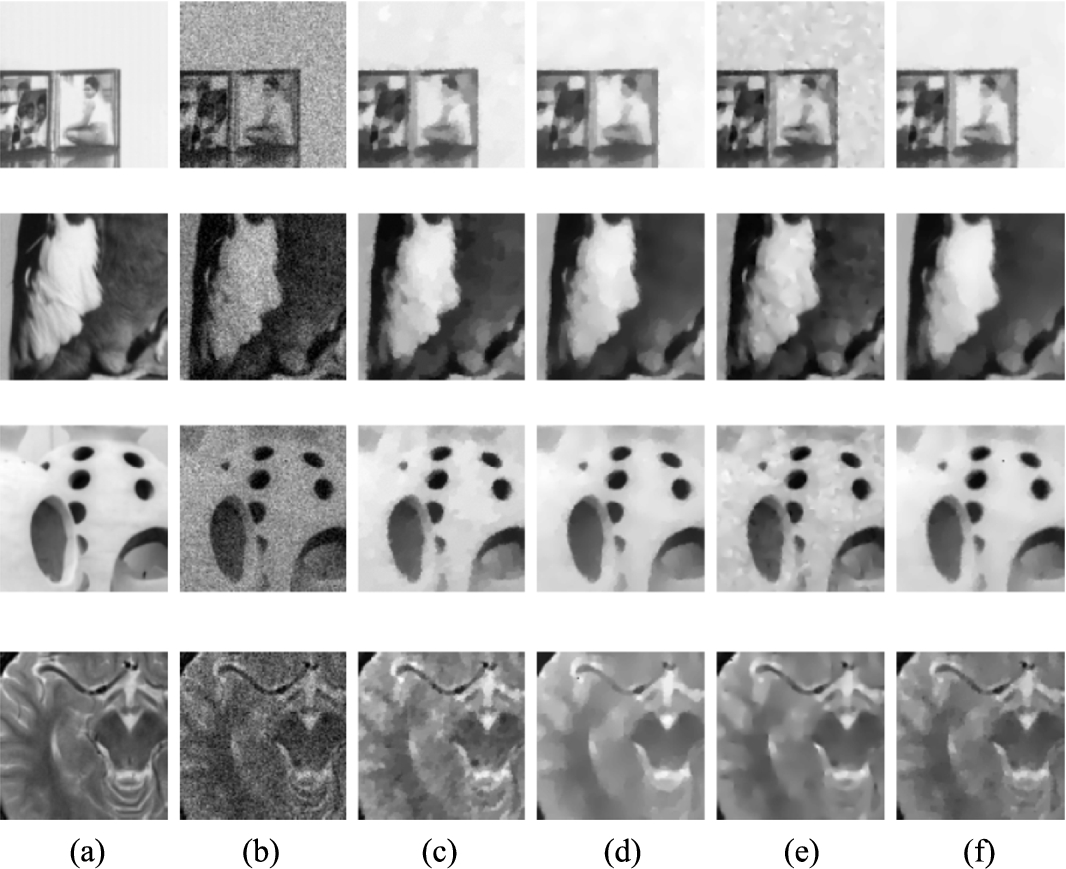
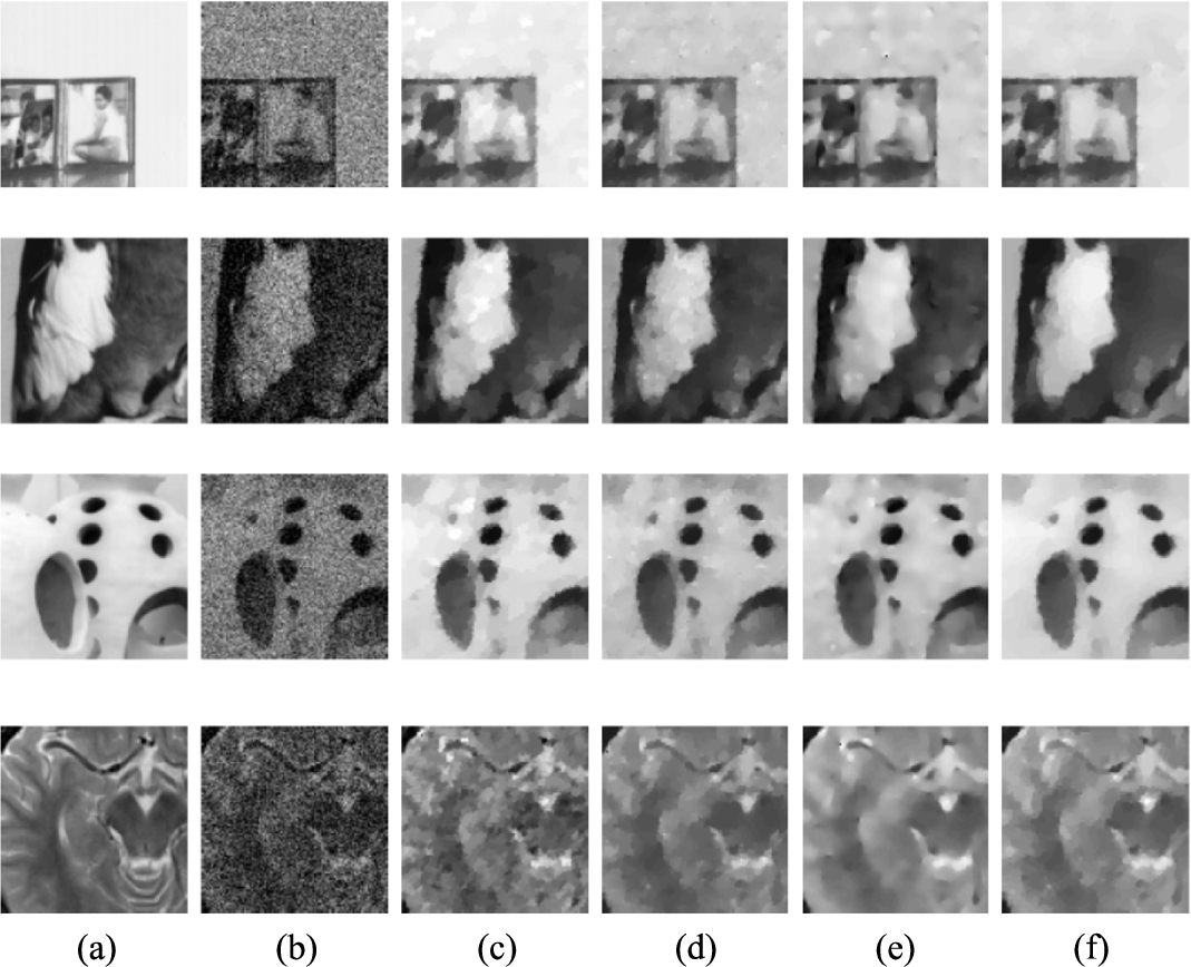
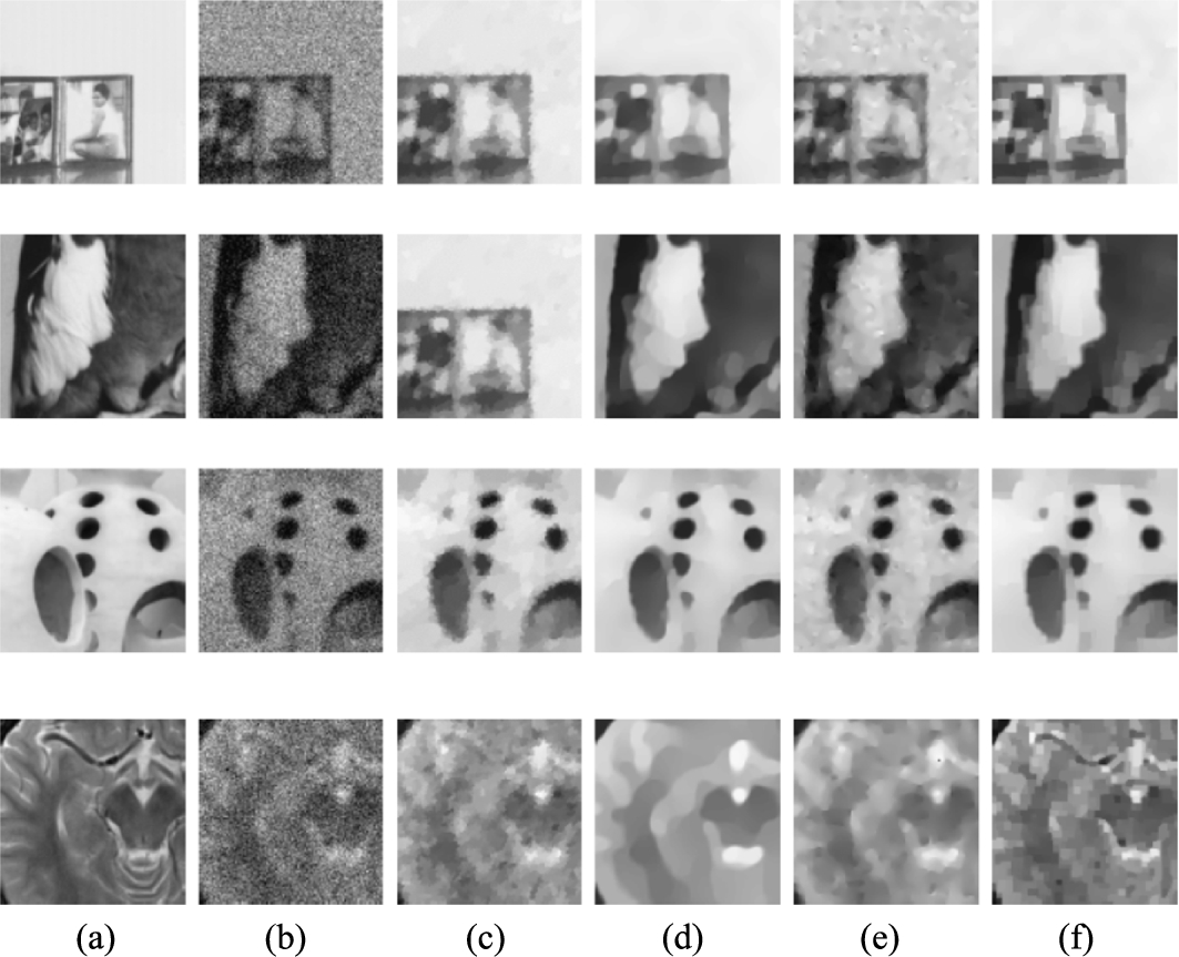
The zoomed-in part of the recovered images in Fig. 2. (a) First column: details of original images; (b) Second column: details of observed images; (c) Third column: details of restored images by TV- method; (d) Fourth column: details of restored images by Bregman method; (e) Fifth column: details of restored images by MS-MPG method; (f) Sixth column: details of restored images by our proposed method.
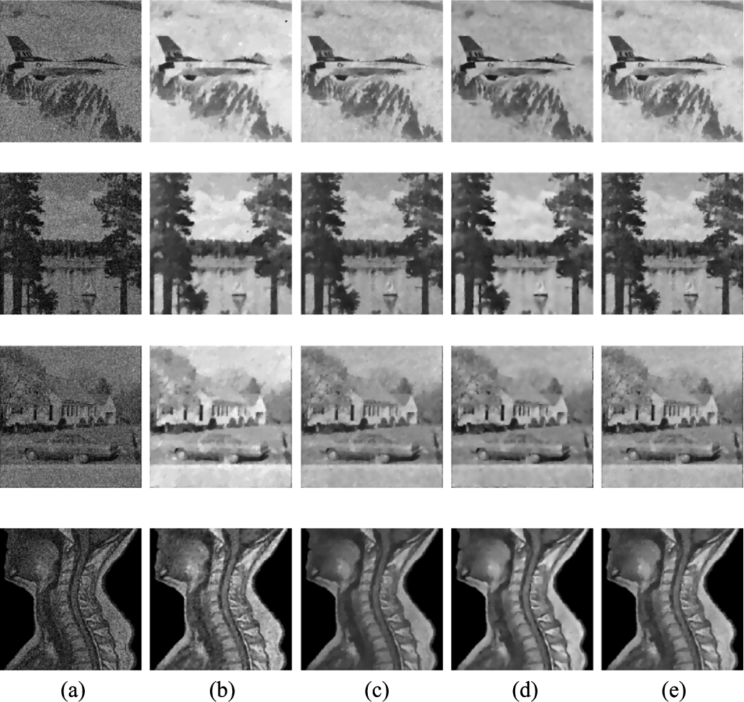
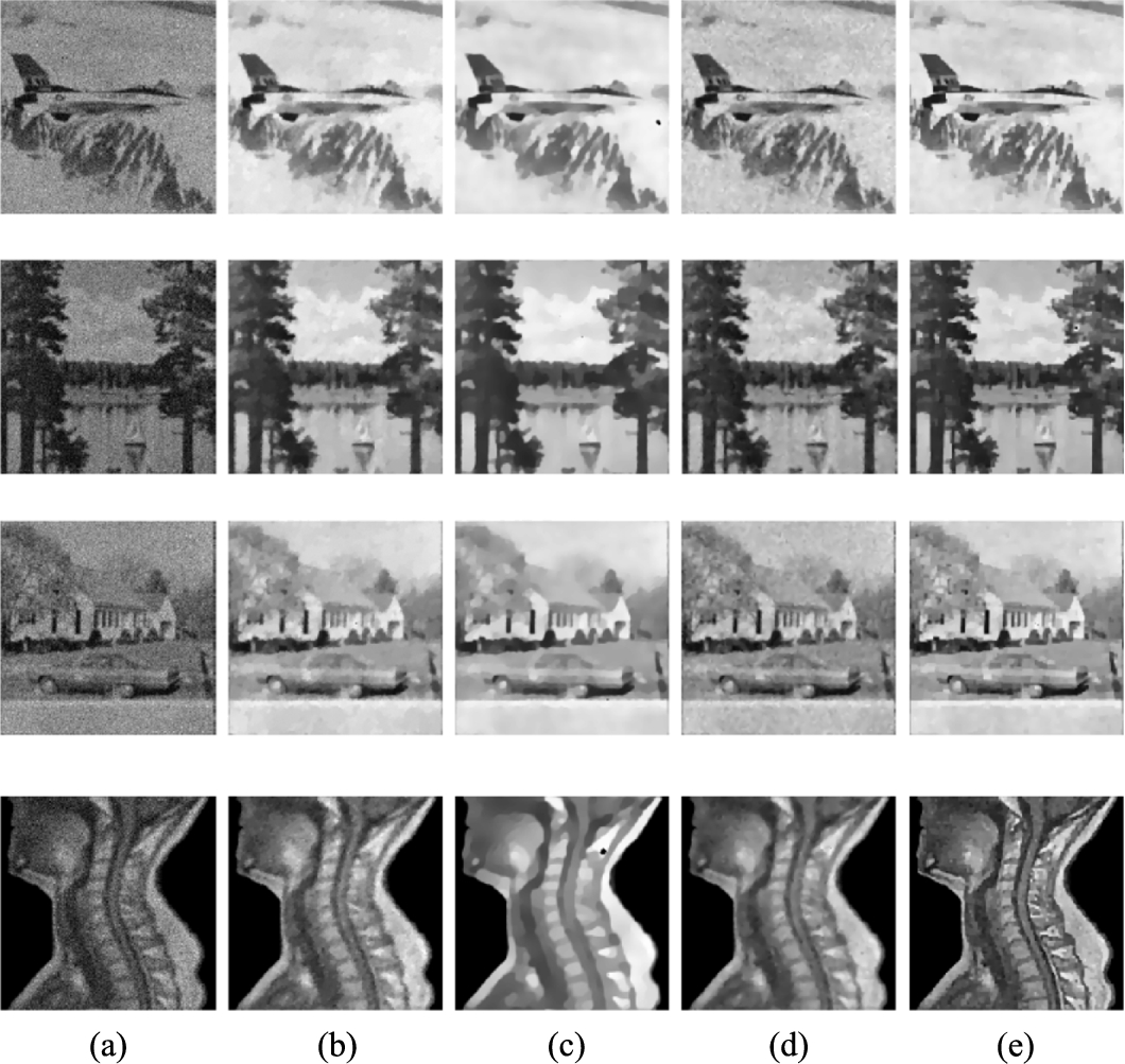
Recovered results for the test images. (a) Noisy image with , , (b) TV , (c) Bregman, (d) MS-MPG, (e) Ours.
Recovered results for the test images. (a) Noisy image with , , (b) TV-, (c) Bregman, (d) MS-MPG, (e) Ours.
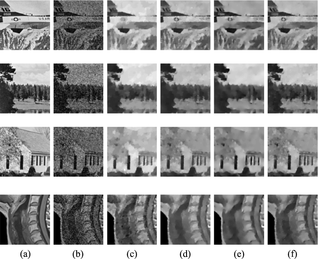
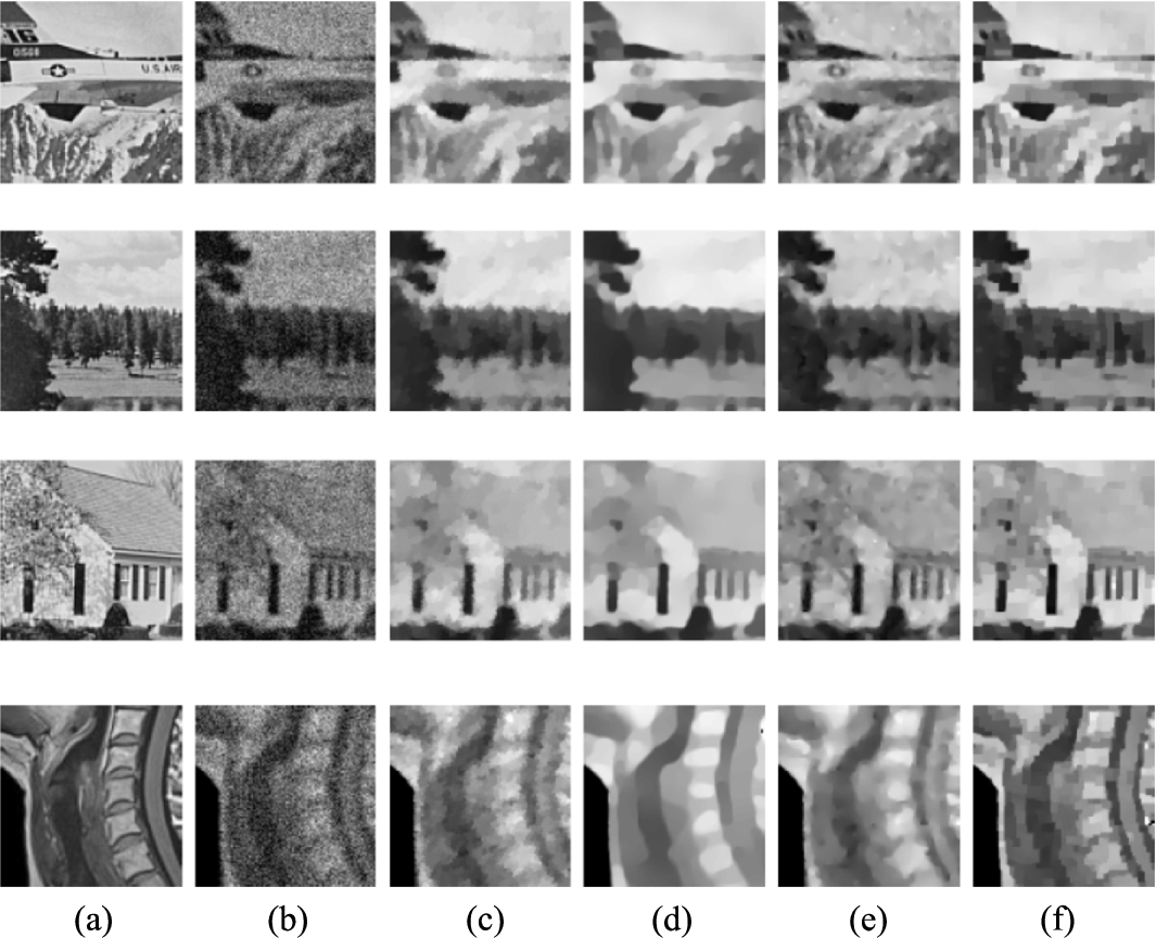
The zoomed-in part of the recovered images in Fig. 4. (a) Details of original images; (b) details of observed images; (c) details of restored images by TV method; (d) details of restored images by Bregman method; (e) details of restored images by MS-MPG method; (f) details of restored images by our proposed method.
The zoomed-in part of the recovered images in Fig. 5. (a) Details of original images; (b) details of observed images; (c) details of restored images by TV method; (d) details of restored images by Bregman method; (e) details of restored images by MS-MPG method; (f) details of restored images by our proposed method.
For a better visual comparison, we have enlarged some details of the restored images in Figs. 3, 6 and 7 (we include the original images in the first column). It can be seen that our method gives even better visual quality than other methods. Table 1 shows the computation time in second(s) of the compared methods for Fig. 2. We see from Table 1 that the computation time of the restored images by the proposed method and the Bregman method is about the same. However, the computational time required by the proposed method is less than that required by the MS-MPG and TV . The comparison metrics PSNR, SSIM are also computed using various noise levels and shown in Table 2 and Table 3. The best values among all the methods are shown in bold. We give the values of the PSNR and SSIM for the noisy and recovered images. The results shown in Tables 1, 2 and 3 prove that the proposed method is convergent and gets higher PSNR and SSIM values than others.
Execution time for different denoising methods (in seconds) with noise level and .
Image
Method
CPU time (s)
TV
4.3449
5.6730
Clock
Bregman
0.9460
0.8212
MS-MPG
4.1465
4.8734
Ours
1.0945
1.1081
TV
5.6229
7.4171
Coco
Bregman
1.0265
0.8414
MS-MPG
4.0844
5.0879
Ours
1.1239
1.2251
TV
4.3096
6.4129
Lamp
Bregman
0.9225
0.9473
MS-MPG
4.1810
4.8758
Ours
0.9431
1.1266
PSNR values and SSIM measures for noisy images and recovered images with .
Image
PSNR
MSSIM
Noisy
TV
Bregman
MS-MPG
Ours
Noisy
TV
Bregman
MS-MPG
Ours
,
Jetplane
18.9416
22.7203
24.1190
24.7848
25.3251
0.4045
0.7061
0.7514
0.7511
0.7748
Lake
19.6413
21.3675
22.5906
22.9972
24.4798
0.5235
0.6360
0.6812
0.7069
0.7603
Aerial
17.4471
18.9550
19.5840
19.3051
19.8806
0.5582
0.5083
0.5808
0.5711
0.7130
Clock
18.3852
24.6040
25.7945
24.8844
26.1201
0.2997
0.8339
0.8822
0.7796
0.8970
Car
19.1385
21.4694
22.1559
22.8793
24.0620
0.4848
0.6106
0.6542
0.6804
0.7256
Coco
16.9119
20.4242
20.4215
20.3426
20.6539
0.2755
0.8551
0.8798
0.8296
0.8950
Lamp
17.8770
24.2808
24.3594
24.1062
24.6339
0.2446
0.8522
0.8891
0.7889
0.8985
Poulina
18.8381
25.2567
25.7203
25.9781
26.0653
0.3250
0.7648
0.7934
0.7982
0.8074
Spine
21.0004
25.2561
24.6855
25.5349
26.1010
0.6180
0.7925
0.7763
0.7967
0.8206
Head
21.7787
24.3567
26.2348
26.9061
27.0979
0.6324
0.8033
0.8043
0.8273
0.8400
Average
18.9960
22.8691
23.5666
23.7719
24.4420
0.4366
0.7363
0.7693
0.7530
0.8132
,
Jetplane
16.7150
22.2033
23.4915
23.6918
24.1415
0.3320
0.6761
0.7248
0.6959
0.7320
Lake
17.2574
20.8215
22.0827
22.2260
23.0442
0.4384
0.6021
0.6732
0.6709
0.7040
Aerial
15.8006
18.7671
19.2795
19.1060
19.4706
0.4622
0.4594
0.5740
0.5139
0.6472
Clock
16.4619
24.2165
25.3645
24.2371
25.7740
0.2440
0.8105
0.8601
0.8186
0.8805
Car
16.8589
20.9512
21.7735
22.1269
22.7608
0.4015
0.5809
0.6402
0.6338
0.6727
Coco
15.4193
20.3398
20.4109
20.1332
20.5488
0.2181
0.8265
0.8599
0.7741
0.8789
Lamp
16.0461
23.8972
23.9090
23.5169
24.3063
0.1964
0.8225
0.8695
0.7210
0.8799
Poulina
16.6627
24.9195
25.2709
25.2753
25.4142
0.2452
0.7346
0.7659
0.7491
0.7739
Spine
18.5582
23.7301
24.4015
24.3122
24.9272
0.5378
0.7418
0.7689
0.7521
0.7794
Head
19.3512
24.549
25.4199
25.8356
25.9893
0.5588
0.7567
0.7836
0.7854
0.7991
Average
16.9131
22.4395
23.1404
23.0461
23.6377
0.3634
0.7011
0.7520
0.7115
0.7748
PSNR values and SSIM measures for noisy images and recovered images with with .
Image
PSNR
MSSIM
Noisy
TV
Bregman
MS-MPG
Ours
Noisy
TV
Bregman
MS-MPG
Ours
,
Jetplane
14.0929
21.4515
22.5116
22.3705
22.8057
0.2570
0.6396
0.6482
0.6730
0.6854
Lake
14.7190
20.1480
20.9885
20.7335
21.5586
0.3488
0.5567
0.5987
0.5945
0.6325
Aerial
13.9091
18.7122
18.9386
18.6929
19.2898
0.3465
0.4036
0.5296
0.3801
0.5635
Clock
13.9941
23.7554
24.7607
24.3166
25.0682
0.1866
0.7759
0.7865
0.7931
0.8439
Car
14.2393
20.3390
20.8993
20.8988
21.4920
0.3124
0.5417
0.5723
0.5709
0.5864
Coco
13.4373
19.9609
19.9082
20.0459
20.2665
0.1573
0.7969
0.7815
0.8218
0.8535
Lamp
13.6235
23.3118
23.2870
23.4892
23.6101
0.1466
0.7898
0.7823
0.8067
0.8568
Poulina
14.1692
24.2429
24.8768
24.8704
24.9272
0.1804
0.6901
0.7169
0.7252
0.7316
Spine
16.0910
22.749
23.3981
23.3266
23.5011
0.4597
0.6821
0.7286
0.7153
0.7308
Head
16.9718
23.667
24.2991
24.2780
24.4763
0.4970
0.7059
0.7494
0.7284
0.7550
Average
14.5247
21.8338
22.3868
22.3022
22.6996
0.2892
0.6582
0.6894
0.6809
0.7240
,
Image
Noisy
TV
Bregman
MS-MPG
Ours
Noisy
TV
Bregman
MS-MPG
Ours
Jetplane
11.4314
20.5604
21.0317
21.2727
21.3729
0.1911
0.5883
0.5208
0.6247
0.6319
Lake
12.0450
19.3676
19.7789
19.9102
20.0911
0.2441
0.5053
0.5209
0.5526
0.5545
Aerial
11.6216
18.4021
18.9001
18.5632
19.1482
0.2425
0.3435
0.4216
0.3518
0.4362
Clock
11.4506
22.9914
23.6737
23.4250
24.3187
0.1365
0.7297
0.6387
0.7298
0.8123
Car
11.5354
19.6031
19.8705
20.1081
20.2498
0.2163
0.4898
0.4776
0.5254
0.5311
Coco
11.1477
19.6694
19.1809
19.7580
19.8315
0.1149
0.7432
0.6010
0.7628
0.8227
Lamp
11.1182
22.6734
22.1005
22.8145
22.9551
0.1014
0.7341
0.6151
0.7430
0.8263
Poulina
11.5927
23.4904
23.8398
23.8808
24.0040
0.1257
0.6353
0.6106
0.6818
0.6960
Spine
13.4551
20.8085
21.9682
22.0129
22.1122
0.3844
0.6115
0.6493
0.6548
0.6658
Head
14.3442
22.4799
22.4954
22.5105
22.9698
0.4370
0.6445
0.6890
0.6853
0.6991
Average
11.9742
21.0046
21.2840
21.4256
21.7053
0.2194
0.6025
0.5745
0.6312
0.6676
Image Deblurring and Denoising
In this section, we perform image denoising and delurring simultaneously. In our simulation, we use the Gaussian blur with a window size , and standard deviation of 1. After the blurring operation, we corrupt the images by Possion noise and . As in the previous experiment, we compare our results with those obtained by employing the Bregman method, the MS-MPG and the TV (see recovered results in Figs. 8, 10, and their zoom-in part in Figs. 9, 11).
Recovered results for the test images. (a) Blurring and Noisy image, (b) TV , (c) Bregman, (d) MS-MPG, (e) Our proposed.
The zoomed-in part of the recovered images in Fig. 8. (a) Details of original images; (b) details of observed images; (c) details of restored images by TV method; (d) details of restored images by Bregman method; (e) details of restored images by MS-MPG method; (f) details of restored images by our proposed method.
Recovered results for the test images. (a) Blurring and Noisy image, (b) TV , (c) Bregman, (d) MS-MPG, (e) Our proposed.
The zoomed-in part of the recovered images in Fig. 10. (a) Details of original images; (b) details of observed images; (c) details of restored images by TV method; (d) details of restored images by Bregman method; (e) details of restored images by MS-MPG method; (f) details of restored images by our proposed method.
PSNR values and SSIM measures for noisy and blurring images and recovered images with with , .
Image
PSNR
MSSIM
Noisy
TV
Bregman
MS-MPG
Ours
Noisy
TV
Bregman
MS-MPG
Ours
,
Jetplane
14.9522
18.7079
18.72012
18.0420
19.0029
0.2282
0.6384
0.6600
0.5883
0.6860
Lake
16.0535
19.6419
19.6100
19.6472
20.2675
0.2876
0.5506
0.5449
0.5654
0.6090
Aerial
15.3701
18.3325
18.8549
18.7495
18.9921
0.3107
0.4647
0.4902
0.4960
0.5030
Clock
16.1891
23.2348
23.5898
22.5893
23.7133
0.1761
0.7758
0.8196
0.6575
0.8313
Car
15.5905
19.6202
19.6600
19.3774
20.1486
0.2408
0.5375
0.5486
0.5286
0.5863
Coco
15.3829
20.1479
20.1762
19.0025
20.3572
0.1410
0.8082
0.8468
0.7524
0.8608
Lamp
15.9477
23.4005
23.6315
21.6657
23.7635
0.1296
0.8001
0.8597
0.6919
0.8679
Poulina
15.3475
19.5518
19.6801
20.2705
20.4392
0.1710
0.6871
0.7099
0.6923
0.7205
Spine
16.0476
19.1907
18.6797
18.8847
19.3544
0.3865
0.5694
0.5832
0.6051
0.6286
Head
14.9812
16.7888
16.6991
16.6044
18.3481
0.4590
0.6352
0.6562
0.6711
0.7061
Average
15.5862
19.8617
19.9301
19.4833
20.4387
0.2531
0.6467
0.6719
0.6249
0.6999
In Table 4, we give the values of the PSNR and SSIM for different images and different variational methods. The best values among all the methods are shown in bold. Comparing the values of the PSNR and SSIM, we can clearly see that our method outperforms the others even in presence of blur.
Conclusion
In this paper, we have studied a fast total variation minimization method for image restoration. We propose an adaptive model for mixed Poisson–Gaussion noise removal. It is proved that the adaptive model is strictly convex. Then, we have employed split Bregman method to solve the proposed minimization problem. Our experimental results have shown that the quality of restored images by the proposed method are competitive with those restored by the existing total variation restoration methods. The most important contribution is that the proposed algorithm is very efficient.
Footnotes
Coming from http://www.imageprocessingplace.com and , accessed 25/03/2019.
Acknowledgements
The authors would like to thank professor S.D. Dvoenko and professor A.V. Kopylov, Tula State University, Tula, Russia, for their advice and comments.
References
1.
AubertG.AujolJ. (2008). A variational approach to remove multiplicative noise. SIAM Journal on Applied Mathematics, 68(4), 925–946.
2.
BarcelosC.A.Z.ChenY. (2000). Heat flows and related minimization problem in image restoration. Computers & Mathematics with Applications, 39(5–6), 81–97.
3.
BoydS.ParikhN.ChuE.PeleatoB.EcksteinJ. (2010). Distributed optimization and statistical learning via the alternating direction method of multipliers. Foundations and Trends in Machine Learning, 3, 1–122.
4.
CalatroniL.De Los ReyesJ.C.SchönliebC.B. (2017). Infimal convolution of data discrepancies for mixed noise removal. SIAM Journal on Imaging Sciences, 10(3), 1196–1233.
5.
ChambolleA. (2004). An algorithm for total variation minimization and applications. Journal of Mathematical Imaging and Vision, 20, 89–97.
6.
ChambolleA.CasellesV.NovagaM.CremersD.PockT. (2010). An introduction to total variation for image analysis. In: Theoretical Foundations and Numerical Methods for Sparse Recovery, Radon Series on Computational and Applied Mathematics, Vol. 9, pp. 263–340.
7.
ChanT.F.ShenJ. (2005). Image Processing and Analysis: Variational, PDE, Wavelet, and Stochastic Methods. Society for Industrial and Applied Mathematics. 400 pp.
8.
ChouzenouxE.JezierskaA.PesquetJ.C.TalbotH. (2015). A convex approach for image restoration with exact Poisson–Gaussian likelihood. SIAM Journal on Imaging Sciences, 8(4), 2662–2682.
9.
De Los ReyesJ.C.SchönliebC.B. (2013). Image denoising: learning the noise model via nonsmooth PDE-constrained optimization. Inverse Problems & Imaging, 7(4), 1183–1214.
10.
DongY.ZengT. (2013). A convex variational model for restoring blurred images with multiplicative noise. SIAM Journal on Imaging Sciences, 6(3), 1598–1625.
11.
FoiA.TrimecheM.KatkovnikV.EgiazarianK. (2008). Practical Poissonian–Gaussian noise modeling and fitting for single-image raw-data. IEEE Transactions on Image Processing, 17(10), 1737–1754.
12.
GoldsteinT.OsherS. (2009). The split Bregman method for L1-regularized problems. SIAM Journal on Imaging Sciences, 2(2), 323–343.
13.
JezierskaA.ChauxC.PesquetJ.C.TalbotH. (2011). An EM approach for Poisson–Gaussian noise modeling In: 19th European Signal Processing Conference (EUSIPCO), Barcelona, Spain, pp. 2244–2248.
14.
KornprobstP.DericheR.AubertG. (1999). Image sequence analysis via partial differential equations. Journal of Mathematical Imaging and Vision, 11, 5–26.
15.
LanzaA.MorigiS.SgallariF.WenY.W. (2014). Image restoration with Poisson–Gaussian mixed noise. Computer Methods in Biomechanics and Biomedical Engineering: Imaging and Visualization, 2(1), 12–24.
16.
Le MontagnerY.AngeliniE.D.Olivo-MarinJ.C. (2014). An unbiased risk estimator for image denoising in the presence of mixed Poisson–Gaussian noise. IEEE Transactions on Image Processing, 23(3), 1255–1268.
17.
LeT.ChartrandR.AsakiT.J. (2007). A variational approach to reconstructing images corrupted by Poisson noise. Journal of Mathematical Imaging and Vision, 27, 257–263.
18.
LiJ.ShenZ.YinR.ZhangX. (2015). A reweighted method for image restoration with Poisson and mixed Poisson–Gaussian noise. Inverse Problems & Imaging, 9(3), 875–894.
LiuL.ChenL.ChenC.L.P.TangY.Y.Man PunC. (2017). Weighted joint sparse representation for removing mixed noise in image. IEEE Transactions on Cybernetics, 47(3), 600–611.
21.
LuisierF.BluT.UnserM. (2011). Image denoising in mixed Poisson–Gaussian noise. IEEE Transactions on Image Processing, 20(3), 696–708.
22.
MakitaloM.FoiA. (2013). Optimal inversion of the generalized Anscombe transformation for Poisson–Gaussian noise. IEEE Transactions on Image Processing, 22(1), 91–103.
23.
MarnissiY.ZhengY.PesqueiJ.C. (2016). Fast variational Bayesian signal recovery in the presence of Poisson–Gaussian noise. In: IEEE International Conference on Acoustics, Speech and Signal Processing (ICASSP), pp. 3964–3968.
PhamC.T.KopylovA. (2015). Multi-quadratic dynamic programming procedure of edge-preserving denoising for medical images. ISPRS-International Archives of the Photogrammetry, Remote Sensing and Spatial Information Sciences, XL–5/W6, 101–106.
26.
PhamC.T.GamardG.KopylovA.TranT.T.T. (2018). An algorithm for image restoration with mixed noise using total variation regularization. Turkish Journal of Electrical Engineering and Computer Sciences, 26(6), 2831–2845.
27.
PhamC.T.TranT.T.T.PhanT.D.K.DinhV.S.PhamM.T.NguyenM.H. (2019). An adaptive algorithm for restoring image corrupted by mixed noise. Journal Cybernetics and Physics, 8(2), 73–82.
SciacchitanoF.DongY.ZengT. (2015). Variational approach for restoring blurred images with Cauchy noise. SIAM Journal on Imaging Sciences, 8(3), 1894–1922.
30.
TranT.T.T.PhamC.T.KopylovA.V.NguyenV.N. (2019). An adaptive variational model for medical images restoration. ISPRS – International Archives of the Photogrammetry, Remote Sensing and Spatial Information Sciences, XLII–2/W12, 219–224.
31.
WangZ.BovikA.C. (2006). Modern Image Quality Assessment, Synthesis Lectures on Image, Video, and Multimedia Processing. Morgan and Claypool Publishers. 156 pp.
32.
WangY.YangJ.YinW.ZhangY. (2008). A new alternating minimization algorithm for total variation image reconstruction. SIAM Journal on Imaging Sciences, 1(3), 248–272.
33.
YanM. (2013). Restoration of images corrupted by impulse noise and mixed Gaussian impulse noise using blind inpainting. SIAM Journal on Imaging Sciences, 6(3), 1227–1245.
34.
ZhangB.FadiliM.J.StarckJ.L.Olivo-MarinJ.C. (2007). Multiscale variance-stabilizing transform for mixed-Poisson–Gaussian processes and its applications in bioimaging. In: IEEE International Conference on Image Processing (ICIP), Vol. 6, 233–236.