An algorithm combining coordinate descent and split Bregman iterative for fractional image denoising model

Abstract

The split Bregman algorithm and the coordinate descent method are efficient tools for solving optimization problems, which have been proven to be effective for the total variation model. We propose an algorithm for fractional total variation model in this paper, and employ the coordinate descent method to decompose the fractional-order minimization problem into scalar sub-problems, then solve the sub-problem by using split Bregman algorithm. Numerical results are presented in the end to demonstrate the superiority of the proposed algorithm.

Introduction

Image denoising is one of the image processing techniques, whose aim is to restore the degraded image g contaminated by noise n to the original image u. An effective denoising technique can remove noise while preserving important image features such as image edge and texture.

$$g=u+n.$$

(1)

Image denoising is an inverse problem. The first denoising model was ill-posed and had no unique stable solution. To solve the ill-posed model, Tikhonov proposed a regularization technique and introduced it into image restoration problem. There are many methods of image restoration at present. Among them, the total variation (TV) model proposed by Rudin et al. ¹ has attracted much attention from scholars. Since the bounded variation functions space allows discontinuities, the edge-preserving ability of TV model is very good.^1–3 However, the staircase effect occurs in the image smooth region. The TV model is formulated as:

$$\underset{u}{min}{\int }_{\mathrm{\Omega }}|\mathrm{\nabla }u|+\frac{\lambda }{2}\parallel u-g{\parallel }^2.$$

(2)

The above model has its advantages and its own temporary insurmountable disadvantages in image processing. In order to make the image processing technology more advanced, many researchers have been trying to study better algorithms. It introduced a novel mesh-free approach using TV regularization and a radial basis function for the numerical approximation of TV-based model to remove the additive noise from the measurements. The author proposed the anisotropic TV model for recovering image corrupted by impulse noise. The L2 fidelity term in formula (2) is replaced by L1. A hybrid regularization model was proposed; the related simulations indicated that the combination scheme performed better than the pure second-order or fourth-order partial differential equations (PDE) models. Engineering researches^4–12 have confirmed that the first-order derivative will increase the high-frequency components such as edge information. For the medium–low-frequency components such as texture details, the fractional derivative can keep the edge better. The theoretical analysis shows that the fractional-order denoising model has good texture retention ability. It extends the integer-order denoising model to the fractional-order and the proposed fractional-order TV model, ⁵ the numerical simulation results proved that the fractional-order TV model has its superiority.

$$\underset{u}{min}{\int }_{\mathrm{\Omega }}|{\mathrm{\nabla }}^{\alpha }u|+\frac{\lambda }{2}\parallel u-g{\parallel }^2.$$

(3)

There are many solutions for minimizing the energy functional problem. Dali Chen et al. ¹³ transformed the minimization problem (3) into a series of simple proximity operators and proposed an effective proximity algorithm. The dual algorithm proposed by Chambolle^14–16 has been applied for rudin osher fatemi (ROF) and lysaker lundervold tai (LLT) models, and the experiments show that this algorithm is faster than the original gradient descent algorithm. An adaptive algorithm for TV-based model of three norms L_q (q = 1/2, 1, 2) has been proposed by Qianshun Chang in the paper, three algorithms are applied for different regions of a given image such that the advantages of each algorithm are adopted. Since the regularization terms of (3) are non-differential,^17,18 the author proposed a projection algorithm for image denoising, they transformed the original problem into a new problem through the sub-gradient and Fenchel conjugate properties.

Tian et al. ¹⁹ proposed a primal–dual algorithm for TV model. This algorithm is more and more advantageous in the CPU time and the number of iterations. The Bregman iterative algorithm proposed in the 1960s for the general pursuit problem. ²⁰ Osher and Cai proposed the linear Bregman algorithm for the compressive sensing problem, Goldstein and Osher ²¹ proposed the split Bregman algorithm for image restoration problem, whose convergence speed is fast.

In this paper, based on the previous work, the coordinate descent method is used to solve the fractional-order TV model and use the split Bregman algorithm for its sub-problem. The rest of paper is organized as follows. In section “Preliminary,” the split Bregman algorithm and the coordinate descent method are introduced; in section “Proposed algorithm,” the proposed algorithm for the fractional-order TV model is proposed. In section “Numerical experiments,” the numerical experiments and results to demonstrate the effectiveness of the proposed method are given. Finally, this paper is concluded in section “Conclusions.”

Preliminary

Split Bregman algorithm and coordinate descent algorithm (CoD) are efficient for solving optimization problems, especially for L1 regulation problem. In this section, two algorithms are briefly introduced.

Split Bregman algorithm

For the general minimization problem

$$\underset{u}{min}J(u)+H(u),$$

(4)

where $J(u)$ and $H(u)$ are convex functions and $H(u)$ is differentiable. Bregman defined the Bregman distance of function J at u and v.^20–22

$$D_J^p(u,v)=J(u)-J(v)-⟨p,u-v⟩$$

where $u,v\in \mathrm{dom}(E)$ , p is the sub-gradient of J at v. Bregman distance is not the distance in general because it does not satisfy the symmetry. Actually, it measures the closeness of u and v. Bregman iterative formula is as follows:

$$\begin{array}{rl}{u}^{k+1}:=& \underset{u}{min}{D}_J^{p^k}(u,u^k)+H(u)\\ =& \underset{u}{min}J(u)-J(u^k)-⟨p^k,u-u^k⟩+H(u),\end{array}$$

(5)

$$p^{k+1}=p^k-\mathrm{\nabla }H(u^{k+1}).$$

(6)

$\mathrm{\nabla }H$ represents the derivative of $H(u)$ .

The energy functional regularization model based on image denoising can be reduced to the following minimization problem:

$$\underset{u}{min}|J(u)|+H(u),$$

(7)

where $|\cdot |$ is $L_1$ normal, $J(u)$ and $H(u)$ are convex functions. Goldstein and Osher^21,22 proposed split Bregman algorithm based on Bregman iterative algorithm. By introducing variable d, the unconstrained (7) equal to the following constrained problem:

$$\underset{u}{min}|d|+H(u),\mathrm{such}\mathrm{that}d=J(u).$$

(8)

Convert (8) into an equivalent unconstrained problem.

$$\underset{u}{min}|d|+H(u)+\frac{\mu }{2}\parallel d-J(u){\parallel }^2.$$

(9)

The $L_1$ and $L_2$ portions of (7) are “de-couple” by split method. Next, let $E(u,d)=|d|+H(u)$ , using the Bregman iterative to solve (9), there would be:

$$\begin{array}{rl}(u^{k+1},d^{k+1})=& \underset{u,d}{min}{D}_J^p(u,u^k,d,d^k)+\frac{\mu }{2}\parallel d-J(u){\parallel }^2\\ =& J(u)+J(d)-J(u^k)-J(d^k)-⟨p_u^k,u-u^k⟩\\ & -⟨p_d^k,d-d^k⟩+\frac{\mu }{2}\parallel d-J(u){\parallel }^2,& \end{array}$$

(10)

$$p_u^{k+1}=p_u^k-\mu (\mathrm{\nabla }J{)}^{\mathrm{T}}(J(u^{k+1})-d^{k+1}),$$

(11)

$$p_d^{k+1}=p_d^k-\mu (d^{k+1}-J(u^{k+1})).$$

(12)

The above split Bregman iteration formulas can be reduced to the following equivalent formulas:

$$(u^{k+1},d^{k+1})=\underset{u,d}{min}|d|+H(u)+\frac{\mu }{2}\parallel d-J(u)-b^k{\parallel }^2,$$

(13)

$$b^{k+1}=b^k+(J(u^{k+1})-d^{k+1}).$$

(14)

The key of split Bregman algorithm is to solve $(u^{k+1},d^{k+1})$ . Similar to the augmented Lagrangian algorithm, the split Bregman algorithm can be split into two subproblems of u and d.

$$\mathrm{Step}1:u^{k+1}=\underset{u}{min}H(u)+\frac{\mu }{2}\parallel d^k-J(u)-b^k{\parallel }^2,$$

(15)

$$\mathrm{Step}2:d^{k+1}=\underset{d}{min}|d|+\frac{\mu }{2}\parallel d-J(u)-b^k{\parallel }^2.$$

(16)

Equation (15) can be solved by Gauss Seidel iteration or Fourier transform, and the solution of equation (16) can be expressed with the shrink operator.

Coordinate descent algorithm

The CoD was proposed in 1998 to solve the linear fitting problem. CoD-based denoising (CoDenoise) algorithm converges fast.^23–25 Its basic idea is to decompose the problem about vectors or matrices into one-dimensional scalar sub-problems.

The following formulation is considered as:

$$\underset{u}{min}f(x)+h(x).$$

(17)

where $x\in R^n$ , $f(x)$ and $h(x)$ are convex functions and $h(x)$ is smooth. Assuming $f(x)$ is separable.

$$f(x)=\sum _{i=1}^n{f}_i(x_i),$$

(18)

Then, the problem (17) can be reduced to solve a series of scalar optimization sub-problem. ²⁶

$$\underset{u}{min}{f}_i(x_i)+h_i(x_i).$$

(19)

The coordinate selection mode, also calls sweeping path-wise, which is the emphasis of CoD method. Applying the effective sweeping path-wise into denoising models can solve problems faster.

Proposed algorithm

The discrete model

Let $X=R^{n\times n}$ , the size of image u is $n\times n$ pixels, the discrete form of the fractional-order TV model is as follows:

$$\underset{u\in X}{min}\sum _{1\le i,j\le n}|{\mathrm{\nabla }}^{\alpha }{u}_{ij}|+\frac{\lambda }{2}{(u_{ij}-g_{ij})}^2.$$

(20)

Based on the idea of coordinate descent, the above denoising problem can be transformed into a series of scalar sub-problems with respect to each pixel $u_{ij}$

$$\underset{u_{ij}}{min}|{\mathrm{\nabla }}^{\alpha }{u}_{ij}|+\frac{\lambda }{2}(u_{ij}-g_{ij}{)}^2,(i,j=1,2,\dots n).$$

(21)

where $|{\mathrm{\nabla }}^{\alpha }{u}_{ij}|$ including two forms is as follows:

$$|{\mathrm{\nabla }}^{\alpha }{u}_{ij}|=\{\begin{array}{cc}|{\mathrm{\nabla }}_x^{\alpha }{u}_{ij}|+|{\mathrm{\nabla }}_y^{\alpha }{u}_{ij}|& \mathrm{anisotropy},\\ \sqrt{{({\mathrm{\nabla }}_x^{\alpha }{u}_{ij})}^2+{({\mathrm{\nabla }}_x^{\alpha }{u}_{ij})}^2}& \mathrm{isotropy}.\end{array}$$

Since the anisotropic $|{\mathrm{\nabla }}^{\alpha }{u}_{ij}|$ is separated, the CoD can be used directly. But the isotropic $|{\mathrm{\nabla }}^{\alpha }{u}_{ij}|$ cannot be decomposed, the algorithm is unfeasible to solve the isotropic problem, Michailovich proposed a multidirectional gradient formulation for this issue. In the following article, we are going to solve the anisotropy problem by using the coordinate descent method and the split Bregman algorithm.

Solving sub-problem

For every anisotropic fractional variable sub-problem, we use the split Bregman algorithm to solve it

$$\underset{u_{ij}}{min}|{\mathrm{\nabla }}_x^{\alpha }{u}_{ij}|+|{\mathrm{\nabla }}_y^{\alpha }{u}_{ij}|+\frac{\lambda }{2}(u_{ij}-g_{ij}{)}^2.$$

(22)

Introduce variables $d_{ij1}$ and $d_{ij1}$ , (22) is equivalent to

$$\begin{array}{rl}& \underset{u_{ij}}{min}|d_{ij1}|+|d_{ij2}|+\frac{\lambda }{2}(u_{ij}-g_{ij}{)}^2\mathrm{s}.\mathrm{t}.d_{ij1}\\ & ={\mathrm{\nabla }}_x^{\alpha }{u}_{ij},d_{ij2}={\mathrm{\nabla }}_y^{\alpha }{u}_{ij}.\end{array}$$

(23)

The equivalent non-constrained problem is considered:

$$\underset{u_{ij}}{min}|d_{ij1}|+|d_{ij2}|+\frac{\lambda }{2}(u_{ij}-g_{ij}{)}^2+\frac{\mu }{2}(d_{ij1}-{\mathrm{\nabla }}_x^{\alpha }{u}_{ij}{)}^2+\frac{\mu }{2}(d_{ij2}-{\mathrm{\nabla }}_y^{\alpha }{u}_{ij}{)}^2$$

(24)

Let $E(u_{ij},d_{ij1},d_{ij2})=|d_{ij1}|+|d_{ij2}|+\frac{\lambda }{2}(u_{ij}-g_{ij}{)}^2$ , then the Bregman distance of E at $(u_{ij}^k,d_{ij1}^k,d_{ij2}^k)$ is

$$\begin{array}{rl}{D}_E^p(u_{ij},u_{ij}^k,d_{ij1},d_{ij1}^k,d_{ij2},d_{ij2}^k)& =|d_{ij1}|+|d_{ij2}|+\frac{\lambda }{2}(u_{ij}-g_{ij}{)}^2-|d_{ij1}^k|-|d_{ij2}^k|-\frac{\lambda }{2}(u_{ij}^k-g_{ij}{)}^2-⟨p_{u_{ij}}^k,u_{ij}-u_{ij}^k⟩\\ & -⟨p_{d_{ij1}}^k,d_{ij1}-d_{ij1}^k⟩-⟨p_{d_{ij2}}^k,d_{ij2}-d_{ij2}^k⟩.\end{array}$$

Applying iterative split Bregman, there would be:

$$\begin{array}{rl}(u_{ij}^{k+1},d_{ij1}^{k+1},d_{ij2}^{k+1})& =\arg \underset{u_{ij},d_{ij1},d_{ij2}}{min}{D}_E^p(u_{ij},u_{ij}^k,d_{ij1},d_{ij1}^k,d_{ij2},d_{ij2}^k)\\ & +\frac{\mu }{2}(d_{ij1}-{\mathrm{\nabla }}_x^{\alpha }{u}_{ij}{)}^2+\frac{\mu }{2}(d_{ij2}-{\mathrm{\nabla }}_y^{\alpha }{u}_{ij}{)}^2.\end{array}$$

(25)

$$\begin{array}{rl}{p}_{u_{ij}}^{k+1}=& p_{u_{ij}}^k+{\mathrm{\nabla }}_{u_{ij}}H(u_{ij},d_{ij1},d_{ij2})\\ p_{d_{ij1}}^{k+1}=& p_{d_{ij1}}^k+{\mathrm{\nabla }}_{d_{ij1}}H(u_{ij},d_{ij1},d_{ij2})\\ p_{d_{ij2}}^{k+1}=& p_{d_{ij2}}^k+{\mathrm{\nabla }}_{d_{ij2}}H(u_{ij},d_{ij1},d_{ij2}).\end{array}$$

(26)

where $H(u_{ij},d_{ij1},d_{ij2})=\frac{\mu }{2}(d_{ij1}-{\mathrm{\nabla }}_x^{\alpha }{u}_{ij}{)}^2+\frac{\mu }{2}(d_{ij2}-{\mathrm{\nabla }}_y^{\alpha }{u}_{ij}{)}^2.$ equations (24) and (25) are equivalent to:

$$(u_{ij}^{k+1},d_{ij1}^{k+1},d_{ij2}^{k+1})=\arg \underset{u_{ij},d_{ij1},d_{ij2}}{min}|d_{ij1}|+|d_{ij2}|+\frac{\lambda }{2}(u_{ij}-g_{ij}{)}^2+\frac{\mu }{2}(d_{ij1}-{\mathrm{\nabla }}_x^{\alpha }{u}_{ij}-b_{ij1}^k{)}^2+\frac{\mu }{2}(d_{ij2}-{\mathrm{\nabla }}_y^{\alpha }{u}_{ij}-b_{ij2}^k{)}^2$$

(27)

$$b_{ij1}^{k+1}=b_{ij1}^k+({\mathrm{\nabla }}_x^{\alpha }{u}_{ij}^{k+1}-d_{ij1}^{k+1})$$

(28)

$$b_{ij2}^{k+1}=b_{ij2}^k+({\mathrm{\nabla }}_y^{\alpha }{u}_{ij}^{k+1}-d_{ij2}^{k+1})$$

(29)

where ${\mathrm{\nabla }}_x^{\alpha }{u}_{ij}$ and ${\mathrm{\nabla }}_y^{\alpha }{u}_{ij}$ are defined as:

$${\mathrm{\nabla }}_x^{\alpha }{u}_{ij}=\sum _{k=0}^{i-1}{(-1)}^k{C}_k^{\alpha }{u}_{i-k,j},{\mathrm{\nabla }}_y^{\alpha }{u}_{ij}=\sum _{k=0}^{j-1}{(-1)}^k{C}_k^{\alpha }{u}_{i,j-k}.$$

Then, the alternating minimization method is used to alternatively minimize one variable while fixing the other one. We consider the following sub-problem of $u_{ij}^{k+1},d_{ij1}^{k+1}$ and $d_{ij2}^{k+1}$ .

$$\begin{array}{rl}{u}_{ij}^{k+1}=& \arg \underset{u_{ij}}{min}\frac{\lambda }{2}(u_{ij}-g_{ij}{)}^2+\frac{\mu }{2}(d_{ij1}^k-{\mathrm{\nabla }}_x^{\alpha }{u}_{ij}-b_{ij1}^k{)}^2\\ & +\frac{\mu }{2}(d_{ij2}^k-{\mathrm{\nabla }}_y^{\alpha }{u}_{ij}-b_{ij2}^k{)}^2\end{array}$$

(30)

In order to compute $d^{k+1}$ , we use the Shrink operator

$$shrink(x,\beta )=\frac{x}{|x|}\ast max(|x|-\beta ,0),$$

$$d_{ij1}^{k+1}=\arg \underset{d_{ij1}}{min}|d_{ij1}|+\frac{\mu }{2}(d_{ij1}-{\mathrm{\nabla }}_x^{\alpha }{u}_{ij}^{k+1}-b_{ij1}^k{)}^2$$

(31)

$$d_{ij2}^{k+1}=\arg \underset{d_{ij2}}{min}|d_{ij2}|+\frac{\mu }{2}(d_{ij2}-{\mathrm{\nabla }}_x^{\alpha }{u}_{ij}^{k+1}-b_{ij2}^k{)}^2$$

(32)

Using the definition of ${\mathrm{\nabla }}_x^{\alpha }{u}_{ij}$ and ${\mathrm{\nabla }}_y^{\alpha }{u}_{ij}$ of above, and according to the function extremum theorem, we get

$$u_{ij}^{k+1}=\frac{\lambda g_{ij}+\mu (d_{ij1}^k-\sum _{k=1}^{i-1}(-1{)}^{\alpha }{C}_k^{\alpha }{u}_{i-k,j}-b_{ij1}^k+d_{ij2}^k-\sum _{k=1}^{j-1}(-1{)}^{\alpha }{C}_k^{\alpha }{u}_{i,j-k}-b_{ij2}^k)}{\lambda +2\mu }$$

(33)

$$d_{ij1}^{k+1}=shrink\left(\sum _{k=0}^{i-1}{(-1)}^{\alpha }{C}_k^{\alpha }{u}_{i-k,j}^{k+1}+b_{ij1}^k,\frac{1}{\mu }\right)$$

(34)

$$d_{ij2}^{k+1}=shrink\left(\sum _{k=0}^{i-1}{(-1)}^{\alpha }{C}_k^{\alpha }{u}_{i,j-k}^{k+1}+b_{ij2}^k,\frac{1}{\mu }\right).$$

(35)

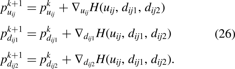
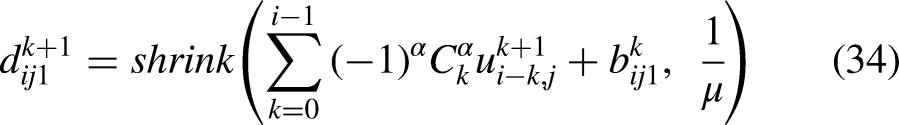
We summarize the algorithm for the fractional variation model as follows; the algorithm has a sequential updating mode:

Algorithm

1. Initialization. Pick $u^0$ and $b_1^0=0,b_2^0=0,d_1^0=0,d_2^0=0$ , choose feasible $\lambda$ and $\mu$ , set $k=0$ .

2. Iteration. For every $i,j=1,2,\dots n$ , Compute $u_{ij}^{k+1}$ , $d_{ij1}^{k+1}$ , $d_{ij2}^{k+1}$ , $b_{ij1}^{k+1}$ and $b_{ij2}^{k+1}$ as (33), (34), (35), (28) and (29).

3. If $u^k$ satisfies the stopping criterion, then we terminate the iteration and output; otherwise, go to step 2.

In this paper, we utilize the fairly naive solution approach which is to discretize in time using the forward Euler finite-difference method and apply second-order finite-difference estimates to approximate the differential operators found:

$$\begin{array}{rl}Set{u}^0:=& f\mathrm{and}\mathrm{for}n=1,2\dots solve:\\ u^{n+1}=& u^n+\mathrm{\Delta }t(A(u^n)+\lambda (f-u^n)),\end{array}$$

(36)

where

$$A(u):=\frac{(u_x^2+{\epsilon }^2)u_{yy}+(u_y^2+{\epsilon }^2)u_{xx}-2u_x{u}_y{u}_{xy}}{{(u_x^2+u_y^2+{\epsilon }^2)}^{3/2}}$$

(37)

We implement each of the differential operators as follows. The first-order derivatives are discretized by the symmetric difference quotient, the second-order derivatives are discretized by the usual second-order difference quotients, while the mixed derivative term is discretized by successively applying the first-order symmetric difference quotients.

Numerical experiments

In this part, we will use some experiment results to show the superiority of the method we proposed.

PSNR, the ratio of the peak signal energy to the average noise energy, is always used to quantify the denoised image, it can be calculated by the following formula:

$$PSNR=10{\log }_{10}\frac{MaxValu{e}^2}{MSE}(\mathrm{dB})=10{\log }_{10}\frac{{255}^2}{MSE}(\mathrm{dB}),$$

(38)

$$MSE=\frac{1}{M\times N}\sum _{i=1}^M\sum _{j=1}^N{[u(i,j)-u_0(i,j)]}^2.$$

(39)

where MSE is the mean variance measure, $M\times N$ is the size of image, $u,u_0$ are the restored image and the original image, respectively. The larger the value of PSNR, the better the image restoration.

Iteration of our model is terminated when the following condition is satisfied:

$$\frac{{\parallel u^{n+1}-u^n\parallel }^2}{{\parallel u^{n+1}\parallel }^2}\le \epsilon ,$$

(40)

where ε is the maximum permissible error, in our experiments we set $\epsilon =0.0001$ .

The used images in these experiments are “Actress” of size 128 × 128, “Building” of size 128 × 128, “Pepper” of size 128 × 128 and “Dog” of size 128 × 128. In addition, the numerical calculations are all accomplished by using MATLAB R2017b.

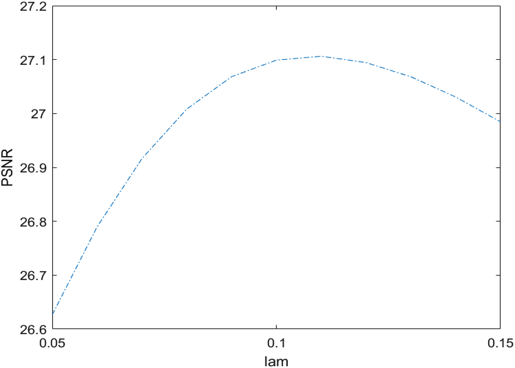
Experiment 1: In this experiment, we try to find the influence of parameters λ and μ on the denoising effect. We add white Gaussian noise with stand variance $\sigma =15$ to “Actress” image. Many experiments show that the model is more effective when λ and μ satisfied 100 to 50 times. Here we show only partial data results, and as is shown in Figure 1, the PSNR is bigger when the λ = 0.1 or so.

Lambda is abbreviated to lam for brevity in the diagrams involved below.

Figure 1.

Line graph of experiment data.

Experiment 2: In this experiment, we set λ = 0.1 and μ = 0.001. The processing effect of the proposed model after 42 iterations of three different noise values $\sigma =20,\sigma =15,\sigma =10$ is compared in Figure 2. Figure 2 shows that our presented model performing well for different variance value, we can get the restoration images which are close to the original image.

Experiment 3: In order to find out the influence of different fractional orders on denoising, in this experiment we add white Gaussian noise with standard variance σ = 15 to “Dog” and implement noise elimination for λ = 0.1 and μ = 0.001. As is shown in Figure 3, Figure 3(c) and (d) are clearer than Figure 3(f) and (g), that is to say, with other variables unchanged, the effect of image restoration seems to get worse and worse as the fractional order increases, we clearly make sure that the better denoising result, the smaller the order. To make the analysis more careful, the results of different fractional orders (α = 1.1, α = 1.2, α = 1.3, α = 1.4, α = 1.5, α = 1.6, α = 1.7, α = 1.8, α = 1.8, α = 1.9) under different iterations (20, 30, 42, 50) are shown in Table 1 (PSNR of restoration image for different iteration numbers) and Figure 4. We find that the PSNR values of this method are almost stable when the image is restored after 30 iterations, these show that the proposed model can achieve a high degree of noise removal very quickly.

Experiment 4: In the previous set of experiments, we find that the algorithm has a good denoising effect when the order is taken as 1.1, and we want this method to process some other images to verify the universal applicability of this method, so we added other images (“Building” of size 128 × 128, “Pepper” of size 128 × 128) in this experiment. All images with noise variance σ = 15 are processed with α = 1.1, λ = 0.07, and μ = 0.0011. After 42 iterations the restoration effect of different images are exhibited in Figure 5 and the PSNR of every image is shown in Table 2. The results show that the model can achieve good recovery effect.

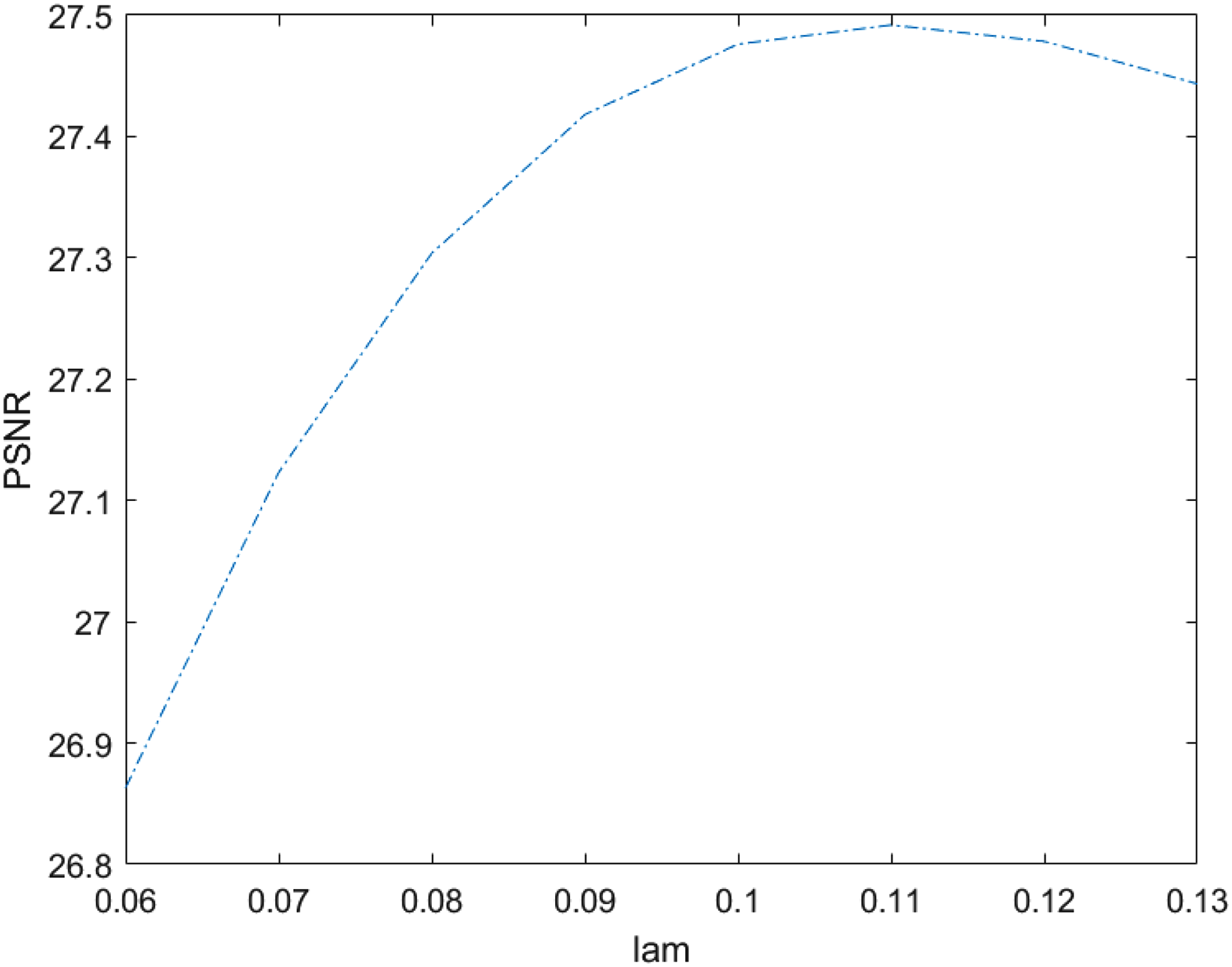
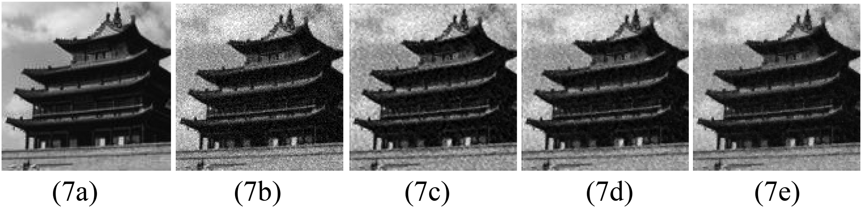
In addition, during the experiment, we have carried out image denoising experiment on picture “Building” in detail; we find that the image “Building” has better restoration effect when the parameters were changed. The conclusion can be achieved more intuitively from Figure 6. Obviously, it is better with λ = 0.11. After that, we set λ = 0.11 and μ = 0.0011, the image “Building” was been recovered for different orders. In the initial experiment, we made the selection about the range of α, we found that the selection of 1–2 were better than those from other data processing, so we chose α as 1–2 in the text for the experiment. What has been shown in Figure 7 and Table 3 is that the results of image restoration seem to get better and better as the fractional order decreases, which is consistent with the deduction of Experiment 3.

Figure 2.

Performance testing. (a) Original image of “Actress”; (b) restoration image for σ = 20; (c) restoration image for σ = 15; (d) restoration image for σ = 10.

Figure 3.

Image restoration effect of different orders. (a) Original image; (b) noisy image; (c) α = 1.1; (d) α = 1.3; (e) α = 1.5; (f) α = 1.7; (g) α = 1.9.

Figure 4.

Corresponding broken line statistical graph.

Figure 5.

The restoration effect of different images. (a) Original image of “Actress”; (b) original image of “Building”; (c) original image of “Pepper”; (d) original image of “Dog”; (e) noisy image of “Actress”; (f) noisy image of “Building”; (g) noisy image of “Pepper”; (h) noisy image of “Dog”; (i) restoration image of “Actress”; (j) restoration image of “Building”; (k) restoration image of “Pepper”; (l) restoration image of “Dog.”

Figure 6.

Line graph of experiment data.

Figure 7.

Image restoration effect of different orders. (a) Original image; (b) noisy image; (c) α = 1.9; (d) α = 1.5; (e) α = 1.1.

Table 1.

Peak signal-to-noise ratio of restoration image for different iteration numbers.

α	1.1	1.2	1.3	1.4	1.5	1.6	1.7	1.8	1.9
20	27.5189	27.7137	27.7360	27.6786	27.5706	27.4138	27.2072	26.9564	26.6706
30	28.2015	28.3539	28.2867	28.1710	28.0312	27.8423	27.5809	27.2459	26.8597
42	28.6025	28.6000	28.3994	28.2387	28.1155	27.9619	27.7171	27.3612	26.9145
50	28.7258	28.5930	28.3127	28.1364	28.0395	27.9291	27.7221	27.3740	26.9104

Table 2.

Peak signal-to-noise ratio (PSNR) of restoration images.

Image	Actress	Building	Pepper	Dog
PSNR	26.3492	26.9380	28.2756	28.4858

Table 3.

Peak signal-to-noise ratio (PSNR) of restoration image for different orders.

α	1.1	1.2	1.3	1.4	1.5	1.6	1.8	1.9
PSNR	27.4919	27.3269	27.1277	26.9679	26.8310	26.6917	26.3318	26.1029
Time (s)	5.973	5.882	5.835	5.871	5.980	31.077	8.051	8.844

Experiment 5: To further analyze the denoising effect of the proposed method, we have made the original image and restored image edge detection analysis, all the experiment results are shown in Figure 8. In order to make the experiment more sufficient, Canny edge detection and the Laplacian of Gaussian edge detection were used to make the edge detection of the original image and the restored image, respectively. By conserving these images we can see that edge detection of the denoised images is very close to edge detection of the original clear images. The conclusion we get is that the method we proposed can well protect the edge of the image when image denoising.

Furthermore, we have made the histogram of gray value of the original image, degraded image, and restoration image in Figure 9. It is clear that the picture gap between Figure 9(a) and (c) is larger than that between Figure 9(a) and (e), the picture gap between Figure 9(b) and (d) is larger than that between Figure 9(b) and (f). This demonstrates that the method we proposed can restore the image perfectly.

Figure 8.

Edge detection analysis. (a) Original image of “Dog”; (b) Canny edge detection image of (8a); (c) Laplacian of Gaussian edge detection image of (8a); (d) Denoised image of “Dog”; (e) Canny edge detection image of (8d); (f) Laplacian of Gaussian edge detection image of (8d); (g) Original image of “Building”; (h) Canny edge detection image of (8g); (i) Laplacian of Gaussian edge detection image of (8g); (j) Denoised image of “Building”; (k) Canny edge detection image of (8j); (l) Laplacian of Gaussian edge detection image of (8j).

Figure 9.

Gray value histogram comparison. (a) Gray value histogram of the original image of “Dog”; (b) Gray value histogram of the original image of “Building”; (c) Gray value histogram of the degraded image of “Dog”; (d) Gray value histogram of the degraded image of “Building”; (e) Gray value histogram of the restored image of “Dog”; (f) Gray value histogram of the restored image of “Building.”

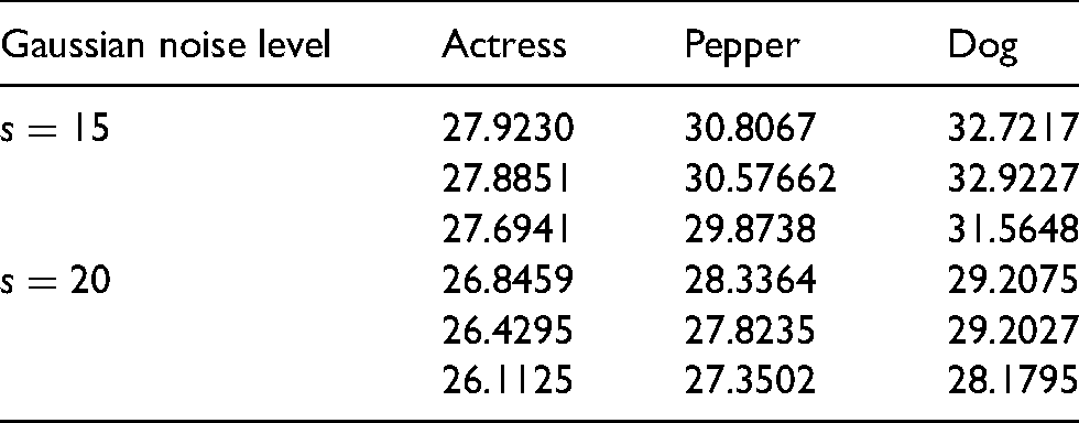
In the fifth experiment, we add different levels of mixed noise to the three images and apply the L1L2/TV model and the coordinate descent algorithm to process the noisy images. The PSNR values of the denoised images are shown in Table 4. The first line in the table shows the PSNR result of the noisy images with only Gaussian noise. The second line shows the PSNR result of the noisy images with only salt and pepper noise. The third line shows the PSNR result of the noisy images with the mixed noise of Gaussian noise and salt and pepper noise. From the table, we observe that the PSNR values of images with different low levels of salt and pepper noise is almost the same at Gaussian noise $s=15$ . Similarly, the same experimental result at Gaussian noise $s=20$ is obtained. The experiments have also shown that the L1L2/TV model and algorithm can effectively remove the mixed noise of Gaussian noise and salt and pepper noise.

Table 4.

Peak signal-to-noise ratio results of the noisy images with different noise level.

Gaussian noise level	Actress	Pepper	Dog
$s=15$	27.9230	30.8067	32.7217
	27.8851	30.57662	32.9227
	27.6941	29.8738	31.5648
$s=20$	26.8459	28.3364	29.2075
	26.4295	27.8235	29.2027
	26.1125	27.3502	28.1795

Table 5.

Peak signal-to-noise ratio (PSNR) results of the noisy images between the two methods.

		The decent method (C)	The coordinate decent method (D)
TOYS	Times	43	52
	PSNR	21.8810	22.6923
	Time (s)	28.712811	15.173902

Experiment 6: PSNR comparisons between the coordinate descent method and the common gradient descent can show the advantages of the coordinate decent method. In the following experiment, we set λ = 0.2 and μ = 0.002. The processing effect of the proposed model after 52 iterations of noise values $\sigma =20$ is compared in Figure 10. Table 5 shows that our presented model performing better between the coordinate decent method and the common gradient descent, we can get the restoration images which are close to the original image.

Conclusions

In this paper, we propose an algorithm for fractional TV model, and employ the coordinate descent method to decompose the fractional-order minimization problem into scalar sub-problems, and then solve it by using split Bregman algorithm. The split Bregman algorithm and the coordinate descent method are combined. The proposed algorithm divides the problem into sub-problems to solve, which reduces the difficulty of the problem. The final experimental results show that the proposed algorithm is effective for image denoising, but there is still space for improvement in discretization and programming, we also believe that this method will show more and more superiority based on continuous improvement.

Figure 10.

The restoration effect of different decent methods. (a) Original image of “Toys”; (b) image of Gaussian noises; (c) denoised image with the decent method; (d) denoised image with the coordinate decent method.