Performance of relaxed iterative methods for image deblurring problems

Abstract

In this paper, we consider performance of relaxation iterative methods for four types of image deblurring problems with different regularization terms. We first study how to apply relaxation iterative methods efficiently to the Tikhonov regularization problems, and then we propose how to find good preconditioners and near optimal relaxation parameters which are essential factors for fast convergence rate and computational efficiency of relaxation iterative methods. We next study efficient applications of relaxation iterative methods to Split Bregman method and the fixed point method for solving the L1-norm or total variation regularization problems. Lastly, we provide numerical experiments for four types of image deblurring problems to evaluate the efficiency of relaxation iterative methods by comparing their performances with those of Krylov subspace iterative methods. Numerical experiments show that the proposed techniques for finding preconditioners and near optimal relaxation parameters of relaxation iterative methods work well for image deblurring problems. For the L1-norm and total variation regularization problems, Split Bregman and fixed point methods using relaxation iterative methods perform quite well in terms of both peak signal to noise ratio values and execution time as compared with those using Krylov subspace methods.

Introduction

Image deblurring is the process of restoring or estimating the true image from the observed blurred and noisy image. There are many mathematical models which have been proposed to solve image deblurring problems. In this paper, we consider four types of image deblurring problems which are expressed as the following minimization problems

$$\underset{x\in {\mathbb{R}}^N}{\min }\left\{{\Vert \mathit{Ax}-b\Vert }_2^2+{\delta }^2{\Vert \mathit{Dx}\Vert }_2^2\right\}$$

(1)

$$\underset{x\in {\mathbb{R}}^N}{\min }\left\{\frac{1}{2}{\Vert \mathit{Ax}-b\Vert }_2^2+\mu {\Vert \mathit{Dx}\Vert }_1\right\}$$

(2)

$$\underset{x\in {\mathbb{R}}^N}{\min }\left\{\frac{1}{2}{\Vert \mathit{Ax}-b\Vert }_2^2+\mu \mathit{TV}(x)\right\}$$

(3)

$$\underset{x\in {\mathbb{R}}^N}{\min }\left\{\frac{1}{2}{\Vert \mathit{Ax}-b\Vert }_2^2+\frac{\alpha }{2}{\Vert x\Vert }_2^2+\mu \mathit{TV}(x)\right\}$$

(4)

where α > 0, δ > 0, and μ > 0 are regularization parameters, $x\in {\mathbb{R}}^N$ and $b\in {\mathbb{R}}^N$ represent the original and observed images, respectively, $A\in {\mathbb{R}}^{N\times N}$ is a blurring matrix, D is a finite difference approximation matrix corresponding to the first- or second-order partial derivative operators,^1,2 ${\Vert ·\Vert }_2$ denotes the L2-norm, ${\Vert ·\Vert }_1$ denotes the L1-norm, TV(x) stands for the discrete total variation (TV) of x, the first terms of ${\Vert \mathit{Ax}-b\Vert }_2^2$ are called the data-fitting terms, and the second terms such as ${\Vert \mathit{Dx}\Vert }_2^2,{\Vert \mathit{Dx}\Vert }_1$ , and TV(x) are called the regularization (or penalty) terms. Throughout the paper, the minimization problem (1) is called the Tikhonov regularization problem, (2) is called the L1-norm regularization problem, and (3) and (4) are called the TV regularization problems.^3,4

Notice that the blurring matrix A is determined by the point spread function (PSF) and the boundary condition imposed outside of the image. In this paper, we only use the reflexive boundary condition, which means that the scene outside the image boundaries is a mirror image of the scene inside the image boundaries.

Let the operator vec denote an operator which transforms an m × n matrix C into a long vector c of size N = m n by stacking the columns of the matrix C from left to right, i.e. $c=\mathit{vec}(C)\in {\mathbb{R}}^N$ . Let the operator array denote the inverse operator of vec, i.e. $C=\mathit{array}(c)\in {\mathbb{R}}^{m\times n}$ . In this paper, we only consider the case of TV(x) which is the isotropic TV of x. In other words, if we let $X=\mathit{array}(x)\in {\mathbb{R}}^{m\times n}$ , then TV (x) = TV (X) is defined by

$$\mathit{TV}\left(x\right)=\mathit{TV}\left(X\right)={\Vert \nabla X\Vert }_{\mathit{itv}}={\displaystyle \sum _{i=1}^m{\displaystyle \sum _{j=1}^n{\Vert \left(\begin{array}{c}{\left({\nabla }_{s}X\right)}_{i,j}\\ {\left({\nabla }_{t}X\right)}_{i,j}\end{array}\right)\Vert }_2}}$$

where

$$\begin{array}{c}{\left({\nabla }_{s}X\right)}_{i,j}=\{\begin{array}{ll}{x}_{i+1,j}-x_{i,j},& 1\le i<m\\ 0,& i=m\end{array},\\ {\left({\nabla }_{t}X\right)}_{i,j}=\{\begin{array}{ll}{x}_{i,j+1}-x_{i,j},& 1\le j<n\\ 0,& j=n\end{array}\end{array}$$

Four types of image deblurring problems (1) to (4) usually use Krylov subspace iterative methods to solve large sparse linear systems arising from their computational processes. The purpose of this paper is to study efficient applications of relaxation iterative methods to four types of image deblurring problems and then to compare their performances with those of Krylov subspace iterative methods. Since convergence rate of relaxation iterative methods depends on the choices of preconditioners and relaxation parameters, it is crucial to find good preconditioners and optimal relaxation parameters. Since the order of blurring matrix A is usually very large, computation of optimal relaxation parameters is very time-consuming. So the novel contribution of this paper is to propose how to choose good preconditioners and near optimal relaxation parameters which provide fast convergence rate and efficient computation for relaxation iterative methods. The relaxation iterative methods to be used in this paper are parameterized Uzawa (PU), ⁵ OPR, ⁶ and generalized symmetric SOR (GSSOR)^7,8 methods which have been proposed for solving singular saddle point problems, and the Krylov subspace method to be used is the preconditioned LSQR (PLSQR) method.^9,10

This paper is organized as follows. In the next section, we briefly review relaxation iterative methods for solving saddle point problems. In the “Relaxation iterative methods for Tikhonov regularization problem” section, we study an application of relaxation iterative methods to the Tikhonov regularization problem (1) with three cases of regularization matrices D. In the “L1-norm regularization problem using relaxation iterative methods” section, we study an application of relaxation iterative methods to Split Bregman method ¹¹ for solving the L1-norm regularization problem (2) with three cases of D described in the “Relaxation iterative methods for Tikhonov regularization problem” section. In the “TV regularization problems using relaxation iterative methods” section, we study an application of relaxation iterative methods to Split Bregman method for solving the TV regularization problems (3) and (4). In the “Fixed point method using relaxation iterative methods” section, we study an application of relaxation iterative methods to the fixed point method for solving the TV regularization problem (4) which has been proposed in Chen et al. ⁴ In the “Numerical experiments” section, we provide numerical experiments for four types of image deblurring problems to evaluate the efficiency of relaxation iterative methods. This evaluation has been done by comparing performances of relaxation iterative methods with those of the PLSQR method. Lastly, some conclusions are drawn.

Review of relaxation iterative methods for saddle point problems

In this section, we briefly review relaxation iterative methods for solving the following saddle point problem

$$\left(\begin{array}{cc}E& B\\ -B^T& 0\end{array}\right)\left(\begin{array}{c}x\\ y\end{array}\right)=\left(\begin{array}{c}b\\ -g\end{array}\right)$$

(5)

where $E\in {\mathbb{R}}^{p\times p}$ is a symmetric positive definite matrix, and $B\in {\mathbb{R}}^{p\times q}$ is a matrix with p ≥ q. When B has a full column rank, the coefficient matrix of equation (5) is nonsingular and so problem (5) is called a nonsingular saddle point problem. When B is a rank-deficient matrix, the coefficient matrix of equation (5) is singular and so the problem (5) is called a singular saddle point problem. Many relaxation iterative methods for solving singular or nonsingular saddle point problems have been proposed by many authors, such as the SOR-like method, SSOR-like method, generalized SOR, GSSOR, PU, OPR, parameterized inexact Uzawa, generalized PIU, Uzawa-SOR, Uzawa-SSOR, Uzawa-AOR, Uzawa-SAOR, and so on (see literature^{5–8,12–16} and the references therein for more details). All relaxation iterative methods have one, two, or three relaxation parameters which need to be predetermined. Even if some of those methods have explicit formulas for computing optimal relaxation parameters, computation of them is very time-consuming for large size of problems. This is the reason why Krylov subspace methods are usually used for image deblurring problems instead of using relaxation iterative methods. So it is worthwhile to study how to apply relaxation iterative methods efficiently to image deblurring problems, which is the main contribution of this paper.

Relaxation iterative methods for Tikhonov regularization problem

In this section, we study an application of the relaxation iterative methods to the Tikhonov regularization problem (1) for solving image deblurring problems. The best way to solve (1) numerically is to treat it as a least squares problem

$$\underset{x\in {\mathbb{R}}^N}{\min }\left\{{\Vert \left(\begin{array}{c}A\\ \delta D\end{array}\right)x-\left(\begin{array}{c}b\\ 0\end{array}\right)\Vert }_2^2\right\}$$

(6)

which is mathematically equivalent to solving the following linear system

$$\left(A^{T}A+{\delta }^2{D}^{T}D\right)x=A^{T}b$$

(7)

If the size of the original image X = array(x) is m × n, then the size of blurring matrix A is N × N with N = mn, which is very large and sparse when m and n are large. So, the linear system (7), or equivalently the least squares problem (6), is usually solved using Krylov subspace methods such as preconditioned CGLS, PLSQR, and so on.^2,9,10,17,18

Another existing approach for solving the linear system (7) is to solve the following generalized saddle point problem^19,20

$$\left(\begin{array}{cc}{I}_N& A\\ -A^T& {\delta }^2{D}^{T}D\end{array}\right)\left(\begin{array}{c}r\\ x\end{array}\right)=\left(\begin{array}{c}b\\ 0\end{array}\right)$$

(8)

where I is the identity matrix of order N and r = b − Ax. It is easy to see that solving the linear system (7) for x is equivalent to finding x from the generalized singular saddle point problem (8).

In this section, we propose a different approach for solving the linear system (7). Let

$$\tilde{A}=\left(\begin{array}{c}A\\ \delta D\end{array}\right),\tilde{b}=\left(\begin{array}{c}b\\ 0\end{array}\right) \text{ and } \tilde{r}=\tilde{b}-\tilde{A}x=\left(\begin{array}{c}{\tilde{r}}^1\\ {\tilde{r}}^2\end{array}\right)$$

Then, the linear system (7) is equivalent to ${\tilde{A}}^T\tilde{r}=0$ and thus one obtains the following singular saddle point problem

$$\left(\begin{array}{cc}{I}_L& \tilde{A}\\ -{\tilde{A}}^T& 0\end{array}\right)\left(\begin{array}{c}\tilde{r}\\ x\end{array}\right)=\left(\begin{array}{c}\tilde{b}\\ 0\end{array}\right)$$

(9)

where L > N and L is usually 2N or 3N. Hence, solving the linear system (7) for x is equivalent to finding x from the singular saddle point problem (9). Notice that the saddle point problem (9) is easier to solve than the generalized saddle point problem (8). Even if the order of coefficient matrix of equation (9) is larger than that of (8), computational amounts required for solving (9) are almost the same as those for solving (8) by using block structure of 2 × 1 block matrix $\tilde{A}$ .

We now consider how to solve the singular saddle point problem (9) using relaxation iterative methods efficiently. In this paper, we only consider three relaxation iterative methods, PU, OPR, and GSSOR, which have explicit formulas for computing their optimal relaxation parameters. We first introduce three cases of regularization matrices D to be used in the Tikhonov regularization problem (1).

D corresponding to the Laplacian operator −Δ (Case 1)

The first case of D is a finite difference matrix corresponding to the Laplacian −(x_ss + x_tt) of the image X ∈ R ^{m × n} , where x_ss and x_tt denote the second-order partial derivatives in the vertical direction and the horizontal direction, respectively. Then the matrix $D\in {\mathbb{R}}^{N\times N}$ can be expressed as

$$\mathit{Dx}=-\left(x_{\mathit{ss}}+x_{\mathit{tt}}\right)=\left(I_n\otimes D_{2,m}+D_{2,n}\otimes I_m\right)x$$

where $x=\mathit{vec}(X)$ , I_n, and I_m are the identity matrices of order n and m, respectively, and D_{2, m} and D_{2, n} are m × m and n × n matrices obtained by finite difference approximations to the second-order partial derivatives −x_ss and −x_tt. More specifically, when m = 4, the matrix D_{2, m} is given by

$$D_{2,m}=\left[\begin{array}{cccc}1& -1& 0& 0\\ -1& 2& -1& 0\\ 0& -1& 2& -1\\ 0& 0& -1& 1\end{array}\right]$$

D corresponding to the gradient operator ∇ (Case 2)

The second case of D is a finite difference matrix corresponding to the gradient (x_s, x_t) ^T of the image X ∈ R ^{m × n} , where x_s and x_t denote the first-order partial derivatives in the vertical and horizontal directions, respectively.

Let D_{1, m} and D_{1, n} be m × m and n × n matrices obtained by finite difference approximations to the first-order partial derivatives x_s and x_t. That is, when m = 4, the matrix D_{1, m} is given by

$$D_{1,m}=\left[\begin{array}{cccc}-1& 1& 0& 0\\ 0& -1& 1& 0\\ 0& 0& -1& 1\\ 0& 0& 0& 0\end{array}\right]$$

Then the matrix $D\in {\mathbb{R}}^{2N\times N}$ can be expressed as

$$\mathit{Dx}=\left(\begin{array}{c}{x}_s\\ x_t\end{array}\right)=\left(\begin{array}{c}{I}_n\otimes D_{1,m}\\ D_{1,n}\otimes I_m\end{array}\right)x=\left(\begin{array}{c}{D}_s\\ D_t\end{array}\right)x$$

where $D_s=I_n\otimes D_{1,m}$ and $D_t=D_{1,n}\otimes I_m$ .

D corresponding to differential operator −(x_ss, x_tt) ^T (Case 3)

The third case of D is a finite difference matrix corresponding to the differential operator −(x_ss, x_tt) ^T of the image X ∈ R ^{m × n} , where x_ss and x_tt denote the second-order partial derivatives in the vertical and horizontal directions, respectively.

Let D_{2, m} and D_{2, n} be finite difference approximate matrices corresponding to −x_ss and −x_tt which are defined in Case 1. Then the matrix $D\in {\mathbb{R}}^{2N\times N}$ can be expressed as

$$\mathit{Dx}=\left(\begin{array}{c}{x}_{\mathit{ss}}\\ x_{\mathit{tt}}\end{array}\right)=\left(\begin{array}{c}{I}_n\otimes D_{2,m}\\ D_{2,n}\otimes I_m\end{array}\right)x=\left(\begin{array}{c}{D}_{\mathit{ss}}\\ D_{\mathit{tt}}\end{array}\right)x$$

where $D_{\mathit{ss}}=I_n\otimes D_{2,m}$ and $D_{\mathit{tt}}=D_{2,n}\otimes I_m$ .

Algorithms for relaxation iterative methods

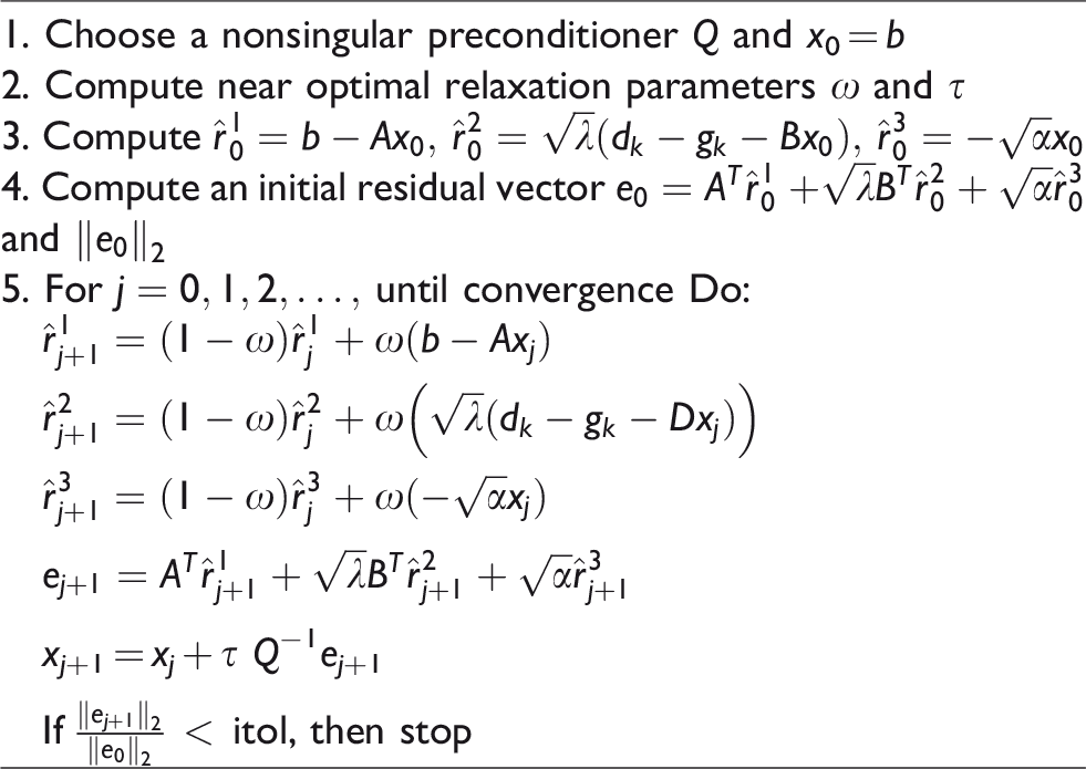
We provide efficient algorithms of relaxation iterative methods for solving the singular saddle point problems (9). Here we only provide an efficient algorithm for PU method since other two relaxation methods (OPR and GSSOR methods) can be done similarly.

Algorithm 1. PU method for solving the saddle point problem (9)

1. Choose a nonsingular preconditioner Q

2. Compute near optimal relaxation parameters ω and τ

3. Choose initial vectors $x_0=b,{\tilde{r}}_0^1=b-A{x}_0,{\tilde{r}}_0^2=-\delta D{x}_0$

4. Compute an initial residual vector $e_0=A^T{\tilde{r}}_0^1+\delta D^T{\tilde{r}}_0^2$ and ${\Vert e_0\Vert }_2$

5. For $k=0,1,2,\dots$  , until convergence Do:

${\tilde{r}}_{k+1}^1=\left(1-\omega \right){\tilde{r}}_k^1+\omega \left(b-A{x}_k\right)$

${\tilde{r}}_{k+1}^2=\left(1-\omega \right){\tilde{r}}_k^2+\omega \left(-\delta D{x}_k\right)$

$e_{k+1}=A^T{\tilde{r}}_{k+1}^1+\delta D^T{\tilde{r}}_{k+1}^2$

$x_{k+1}=x_k+\tau Q^{-1}{e}_{k+1}$

If $\frac{{\Vert e_{k+1}\Vert }_2}{{\Vert e_0\Vert }_2}<\text{tol}$ , then stop

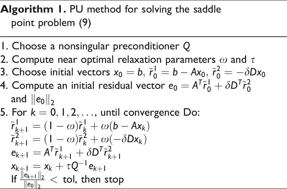
In Algorithm 1, tol denotes the tolerance of stopping criterion which is set to 10⁻² for test problems used in this paper.

Notice that the convergence rate of Algorithm 1 depends upon the choices of a good preconditioner Q and optimal relaxation parameters ω and τ. We first describe how to choose a good nonsingular preconditioner Q efficiently. Based on the theory of relaxation iterative methods, Q is chosen to be a symmetric positive definite matrix which approximates ${\tilde{A}}^T\tilde{A}=A^{T}A+{\delta }^2{D}^{T}D$ . Such a Q can be obtained efficiently by using the following steps

Step 1: Construct symmetric approximation matrices

C^TΛ_aC ≈ A and C^TΛ_dC ≈ D using the DCT2

Step 2: Construct $\tilde{Q}=C^T\left({\left|{\Lambda }_a\right|}^2+{\delta }^2{\left|{\Lambda }_d\right|}^2\right)C$

≈ A^TA + δ²D^TD

Step 3: Let $\Sigma ={\left|{\Lambda }_a\right|}^2+{\delta }^2{\left|{\Lambda }_d\right|}^2=\left({\sigma }_{\mathit{ij}}\right)$ .

If σ_ii < Cut-Off, then σ_ii = 1

Step 4: Construct a symmetric positive definite

preconditioner Q = C^TΣC which modifies the ill-conditioned matrix $\tilde{Q}$ .

Here Λ _a and Λ _d are diagonal matrices, C is the orthogonal two-dimensional discrete cosine transformation matrix, the DCT2 refers to the two-dimensional discrete cosine transformation, and Cut-Off is a positive small value which guarantees the well-conditioned and positive-definite properties of Q. When constructing Q, the matrix C is never computed and only the diagonal matrix Σ is computed. This is because matrix-vector multiplication with C can be easily done using Matlab function dct2 without constructing C. All the diagonal elements of Σ can be easily computed from the corresponding PSFs without constructing A and D. Hence the matrix Q is an efficient preconditioner whose construction and computation with a vector can be done easily without requiring a lot of computational amounts.

We next describe how to choose near optimal relaxation parameters ω and τ of Algorithm 1. Let μ_min and μ_max be the smallest and largest nonzero eigenvalues of the matrix $Q^{-1}{\tilde{A}}^T\tilde{A}=Q^{-1}\left(A^{T}A+{\delta }^2{D}^{T}D\right)$ , respectively. Then the explicit formulas for finding optimal relaxation parameters ω_o and τ_o of PU method ⁵ are given by

$${\omega }_o=\frac{4\sqrt{{\mu }_{\min }{\mu }_{\max }}}{{\left(\sqrt{{\mu }_{\min }}+\sqrt{{\mu }_{\max }}\right)}^2}\text{ and }{\tau }_o=\frac{1}{\sqrt{{\mu }_{\min }{\mu }_{\max }}}$$

(10)

Since the order of A is N = m n which is usually very large, computation of μ_min and μ_max is very time-consuming. Thus, we want to compute near optimal parameters ω and τ instead of computing optimal parameters ω_o and τ_o. Let ν_min and ν_max be the smallest and largest nonzero eigenvalues of the matrix $Q_s^{-1}(A_s^T{A}_s+{\delta }^2{D}_s^T{D}_s)$ , respectively. Here s refers to the order of A_s, Q_s, and $D_s^T{D}_s$ which is much smaller than the order N of A, Q and D^TD. For test problems used in this paper, s is set to $\frac{N}{256}$ , and A_s and D_s are blurring and regularization matrices corresponding to an image of size $\frac{m}{16}\times \frac{n}{16}$ , respectively. Then the near optimal values ω and τ are computed from (10) using ν_min and ν_max instead of using μ_min and μ_max. Since computational time of ν_min and ν_max is much smaller than that of μ_min and μ_max, the near optimal values ω and τ can be computed much faster than the optimal parameters ω_o and τ_o.

L1-norm regularization problem using relaxation iterative methods

In this section, we study an application of relaxation iterative methods to Split Bregman method ¹¹ for solving the L1-norm regularization problem (2) with three cases of D described in the “Relaxation iterative methods for Tikhonov regularization problem” section. Note that the L1-norm regularization problem (2) with Case 2 of D is called the anisotropic TV regularization problem.

We first provide Split Bregman method for solving (2). Let us consider the problem (2) as a constrained minimization problem

$$\underset{x,d\in {\mathbb{R}}^N}{\min }\left\{\frac{1}{2}{\Vert \mathit{Ax}-b\Vert }_2^2+\mu {\Vert d\Vert }_1\right\}\text{such}\text{that}d=\mathit{Dx}$$

(11)

Rather than considering (11), we will consider the following unconstrained minimization problem with a penalty parameter λ > 0

$$\underset{x,d\in {\mathbb{R}}^N}{\min }\left\{\frac{1}{2}{\Vert \mathit{Ax}-b\Vert }_2^2+\mu {\Vert d\Vert }_1+\frac{\lambda }{2}{\Vert d-\mathit{Dx}\Vert }_2^2\right\}$$

(12)

Given x₀ = b and d₀ = g₀ = 0, the alternating Split Bregman method using an auxiliary vector g for solving (12) has the following iteration form

$$x_{k+1}=\underset{x\in {\mathbb{R}}^N}{\text{argmin}}\left\{\frac{1}{2}{\Vert \mathit{Ax}-b\Vert }_2^2+\frac{\lambda }{2}{\Vert d_k-\mathit{Dx}-g_k\Vert }_2^2\right\}$$

(13)

$$d_{k+1}=\underset{d\in {\mathbb{R}}^N}{\text{argmin}}\left\{\mu {\Vert d\Vert }_1+\frac{\lambda }{2}{\Vert d-D{x}_{k+1}-g_k\Vert }_2^2\right\}$$

(14)

$$g_{k+1}=g_k+D{x}_{k+1}-d_{k+1}$$

(15)

These iterations yield the following decoupled subproblems. Finding x_k+1 from subproblem (13) is equivalent to solving the following linear system for x

$$\left(A^{T}A+\lambda D^{T}D\right)x=A^{T}b+\lambda D^T\left(d_k-g_k\right)$$

(16)

Another subproblem (14) can be solved by applying the following shrinkage formula

$$\begin{array}{l}{d}_{k+1}=\text{shrink}\left(D{x}_{k+1}+g_k,\frac{\mu }{\lambda }\right)\\ =\max \left\{|D{x}_{k+1}+g_k|-\frac{\mu }{\lambda }e,0\right\}.*\text{sgn}\left(D{x}_{k+1}+g_k\right)\end{array}$$

(17)

where e is a vector whose elements are all 1 and the operation .* means elementwise multiplications of two vectors.

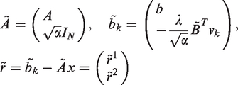
We next propose how to solve the linear system (16) using relaxation iterative methods instead of solving it directly using Krylov subspace methods. Let

$$\begin{array}{l}\widehat{A}=\left(\begin{array}{c}A\\ \sqrt{\lambda }D\end{array}\right),{\widehat{b}}_k=\left(\begin{array}{c}b\\ \sqrt{\lambda }(d_k-g_k)\end{array}\right),\\ \widehat{r}={\widehat{b}}_k-\widehat{A}x=\left(\begin{array}{c}{\widehat{r}}^1\\ {\widehat{r}}^2\end{array}\right)\end{array}$$

Then, the linear system (16) is equivalent to ${\widehat{A}}^T\widehat{r}=0$ and thus one obtains the following singular saddle point problem

$$\left(\begin{array}{cc}{I}_L& \widehat{A}\\ -{\widehat{A}}^T& 0\end{array}\right)\left(\begin{array}{c}\widehat{r}\\ x\end{array}\right)=\left(\begin{array}{c}{\widehat{b}}_k\\ 0\end{array}\right)$$

(18)

where L is 2N or 3N. Finding x from the singular saddle point problem (18) can be done efficiently using relaxation iterative methods. We only provide an efficient algorithm for PU method:

Algorithm 2. PU method for solving the saddle point problem (18)

1. Choose a nonsingular preconditioner Q and x0 = b

2. Compute near optimal relaxation parameters ω and τ

3. Compute ${\widehat{r}}_0^1=b-A{x}_0,{\widehat{r}}_0^2=\sqrt{\lambda }(d_k-g_k-D{x}_0)$

4. Compute an initial residual vector $e_0=A^T{\widehat{r}}_0^1+\sqrt{\lambda }{D}^T{\widehat{r}}_0^2$ and ${\Vert e_0\Vert }_2$

5. For $j=0,1,2,\dots ,$ until convergence Do:

${\widehat{r}}_{j+1}^1=(1-\omega ){\widehat{r}}_j^1+\omega (b-A{x}_j)$

${\widehat{r}}_{j+1}^2=\left(1-\omega \right){\widehat{r}}_j^2+\omega \left(\sqrt{\lambda }\left(d_k-g_k-D{x}_j\right)\right)$

$e_{j+1}=A^T{\widehat{r}}_{j+1}^1+\sqrt{\lambda }{D}^T{\widehat{r}}_{j+1}^2$

$x_{j+1}=x_j+\tau Q^{-1}{e}_{j+1}$

If $\frac{{\Vert e_{j+1}\Vert }_2}{{\Vert e_0\Vert }_2}<\text{itol}$ , then stop

In Algorithm 2, itol denotes the tolerance of stopping criterion which is set to 10⁻³ for test problems used in this paper. The preconditioner Q and near optimal relaxation parameters ω and τ are computed in the same way as was done in the “Relaxation iterative methods for Tikhonov regularization problem” section. The only difference is the value of s which is set to $\frac{N}{64}$ or $\frac{N}{256}$ depending upon the size of images to be deblurred. For test problems used in this paper, $s=\frac{N}{64}$ for small images of size 256 × 256, and $s=\frac{N}{256}$ for large images of size 512 × 512.

Finally, we provide the Split Bregman method using relaxation iterative method for solving the L1-norm regularization problem (2).

Algorithm 3. Split Bregman method for the L1-norm problem (2)

1. Choose regularization parameters λ > 0 and μ > 0

2. Choose x0 = b and d0 = g0 = 0

3. For $k=0,1,2,\dots ,$ until convergence Do:

Solve the singular saddle point problem (18) using Algorithm 2

$d_{k+1}=\text{shrink}\left(D{x}_{k+1}+g_k,\frac{\mu }{\lambda }\right)$

gk+1 = gk + Dxk+1 − dk+1

If $\frac{{\Vert x_{k+1}-x_k\Vert }_2}{{\Vert x_{k+1}\Vert }_2}<\text{otol}$ , then stop

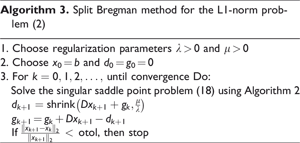
In Algorithm 3, otol denotes the tolerance of stopping criterion which is set to 10⁻³ for test problems used in this paper. When using Algorithm 2, the preconditioner Q and near optimal relaxation parameters ω and τ are computed only once at the first iteration of Algorithm 3. This is because the coefficient matrix (A^TA + λD^TD) is unchanged during the whole iterations.

TV regularization problems using relaxation iterative methods

In this section, we study an application of relaxation iterative methods to Split Bregman method for solving the TV regularization problems (3) and (4). We first provide Split Bregman method for solving problem (3). Problem (3) can be considered as a constrained minimization problem

$$\underset{x\in {\mathbb{R}}^N,d\in {\mathbb{R}}^{2N}}{\min }\left\{\frac{1}{2}{\Vert \mathit{Ax}-b\Vert }_2^2+\mu {\Vert d\Vert }_{\mathit{itv}}\right\}\text{such}\text{that}d=\mathit{Bx}$$

(19)

where ${\Vert d\Vert }_{\mathit{itv}}={\sum }_{i=1}^N{\Vert \left(\begin{array}{c}{\left(d\right)}_i\\ {\left(d\right)}_{N+i}\end{array}\right)\Vert }_2$ , (d) _i denotes the ith component of the vector $d\in {\mathbb{R}}^{2N}$ , and $B\in {\mathbb{R}}^{2N\times N}$ is a finite difference matrix corresponding to Case 2 of D described in the “Relaxation iterative methods for Tikhonov regularization problem” section, i.e. $B={\left(\begin{array}{cc}{I}_n\otimes D_{1,m}^T& D_{1,n}^T\otimes I_m\end{array}\right)}^T$

Rather than considering (19), we will consider the following unconstrained minimization problem with a penalty parameter λ > 0

$$\underset{x\in {\mathbb{R}}^N,d\in {\mathbb{R}}^{2N}}{\min }\left\{\frac{1}{2}{\Vert \mathit{Ax}-b\Vert }_2^2+\mu {\Vert d\Vert }_{\mathit{itv}}+\frac{\lambda }{2}{\Vert d-\mathit{Bx}\Vert }_2^2\right\}$$

(20)

Given x₀ = b and d₀ = g₀ = 0, the alternating Split Bregman method using an auxiliary vector g for solving (20) has the following iteration form

$$x_{k+1}=\underset{x\in {\mathbb{R}}^N}{\text{argmin}}\left\{\frac{1}{2}{\Vert \mathit{Ax}-b\Vert }_2^2+\frac{\lambda }{2}{\Vert d_k-\mathit{Bx}-g_k\Vert }_2^2\right\}$$

(21)

$$d_{k+1}=\underset{d\in {\mathbb{R}}^N}{\text{argmin}}\left\{\mu {\Vert d\Vert }_{\mathit{itv}}+\frac{\lambda }{2}{\Vert d-B{x}_{k+1}-g_k\Vert }_2^2\right\}$$

(22)

$$g_{k+1}=g_k+B{x}_{k+1}-d_{k+1}$$

(23)

Subproblem (21) is equivalent to solving the following linear system for x

$$\left(A^{T}A+\lambda B^{T}B\right)x=A^{T}b+\lambda B^T\left(d_k-g_k\right)$$

(24)

From subproblem (22), $d_{k+1}\in {\mathbb{R}}^{2N}$ can be obtained by using the following generalized shrinkage formula ¹¹ : For each i = 1, 2, … , N

$$\left(\begin{array}{c}{\left(d_{k+1}\right)}_i\\ {\left(d_{k+1}\right)}_{N+i}\end{array}\right)=\max \left\{{\Vert B{G}_i\Vert }_2-\frac{\mu }{\lambda },0\right\}\frac{B{G}_i}{{\Vert B{G}_i\Vert }_2}$$

(25)

where $B{G}_i=\left(\begin{array}{c}{\left(B{x}_{k+1}+g_k\right)}_i\\ {\left(B{x}_{k+1}+g_k\right)}_{N+i}\end{array}\right)\in {\mathbb{R}}^2$ .

Let

$$\begin{array}{l}\widehat{A}=\left(\begin{array}{c}A\\ \sqrt{\lambda }B\end{array}\right),{\widehat{b}}_k=\left(\begin{array}{c}b\\ \sqrt{\lambda }\left(d_k-g_k\right)\end{array}\right),\\ \widehat{r}={\widehat{b}}_k-\widehat{A}x=\left(\begin{array}{c}{\widehat{r}}^1\\ {\widehat{r}}^2\end{array}\right)\end{array}$$

Then, solving the linear system (24) for x is equivalent to finding x from the following singular saddle point problem

$$\left(\begin{array}{cc}{I}_{3N}& \widehat{A}\\ -{\widehat{A}}^T& 0\end{array}\right)\left(\begin{array}{c}\widehat{r}\\ x\end{array}\right)=\left(\begin{array}{c}{\widehat{b}}_k\\ 0\end{array}\right)$$

(26)

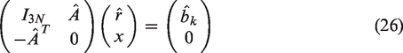
Thus, we want to solve the singular saddle point problem (26), which can be done efficiently using Algorithm 2 with D = B, instead of solving (24) directly using Krylov subspace method.

We next provide Split Bregman method for solving the TV regularization problem (4). In the similar way as was done for (3), one can easily obtain the following iteration form

$$x_{k+1}=\underset{x\in {\mathbb{R}}^N}{\text{argmin}}\{\frac{1}{2}{\Vert \mathit{Ax}-b\Vert }_2^2+\frac{\alpha }{2}{\Vert x\Vert }_2^2+\frac{\lambda }{2}{\Vert d_k-\mathit{Bx}-g_k\Vert }_2^2\}$$

(27)

$$d_{k+1}=\underset{d\in {\mathbb{R}}^N}{\text{argmin}}\left\{\mu {\Vert d\Vert }_{\mathit{itv}}+\frac{\lambda }{2}{\Vert d-B{x}_{k+1}-g_k\Vert }_2^2\right\}{g}_{k+1}=g_k+B{x}_{k+1}-d_{k+1}$$

(28)

We only need to consider the subproblem (27) since (28) is exactly the same as (22). (27) is equivalent to solving the following linear system for x

$$\left(A^{T}A+\lambda B^{T}B+\alpha I_N\right)x=A^{T}b+\lambda B^T\left(d_k-g_k\right)$$

(29)

Let

$$\begin{array}{l}\widehat{A}=\left(\begin{array}{c}A\\ \sqrt{\lambda }B\\ \sqrt{\alpha }{I}_N\end{array}\right),{\widehat{b}}_k=\left(\begin{array}{c}b\\ \sqrt{\lambda }\left(d_k-g_k\right)\\ 0\end{array}\right),\\ \widehat{r}={\widehat{b}}_k-\widehat{A}x=\left(\begin{array}{c}{\widehat{r}}^1\\ {\widehat{r}}^2\\ {\widehat{r}}^3\end{array}\right)\end{array}$$

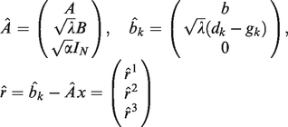
Then, solving the linear system (29) for x is equivalent to finding x from the following nonsingular saddle point problem

$$\left(\begin{array}{cc}{I}_{4N}& \widehat{A}\\ -{\widehat{A}}^T& 0\end{array}\right)\left(\begin{array}{c}\widehat{r}\\ x\end{array}\right)=\left(\begin{array}{c}{\widehat{b}}_k\\ 0\end{array}\right)$$

(30)

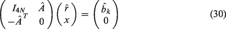
Notice that the coefficient matrix of equation (30) is nonsingular since $\widehat{A}\in {\mathbb{R}}^{4N\times N}$ has full column rank N. It follows that (30) is less ill-conditioned and easier to solve than other singular saddle point problems. Problem (30) can be solved efficiently using relaxation iterative method as follows:

Algorithm 4.

method for solving the saddle point problem (30)

1. Choose a nonsingular preconditioner Q and x0 = b

2. Compute near optimal relaxation parameters ω and τ

3. Compute ${\widehat{r}}_0^1=b-A{x}_0,{\widehat{r}}_0^2=\sqrt{\lambda }\left(d_k-g_k-B{x}_0\right),{\widehat{r}}_0^3=-\sqrt{\alpha }{x}_0$

4. Compute an initial residual vector $e_0=A^T{\widehat{r}}_0^1+\sqrt{\lambda }{B}^T{\widehat{r}}_0^2+\sqrt{\alpha }{\widehat{r}}_0^3$

and ${\Vert e_0\Vert }_2$

5. For $j=0,1,2,\dots ,$ until convergence Do:

${\widehat{r}}_{j+1}^1=\left(1-\omega \right){\widehat{r}}_j^1+\omega \left(b-A{x}_j\right)$

${\widehat{r}}_{j+1}^2=\left(1-\omega \right){\widehat{r}}_j^2+\omega \left(\sqrt{\lambda }\left(d_k-g_k-D{x}_j\right)\right)$

${\widehat{r}}_{j+1}^3=\left(1-\omega \right){\widehat{r}}_j^3+\omega \left(-\sqrt{\alpha }{x}_j\right)$

$e_{j+1}=A^T{\widehat{r}}_{j+1}^1+\sqrt{\lambda }{B}^T{\widehat{r}}_{j+1}^2+\sqrt{\alpha }{\widehat{r}}_{j+1}^3$

xj+1 = xj + τ Q−1ej+1

If $\frac{{\Vert e_{j+1}\Vert }_2}{{\Vert e_0\Vert }_2}<\text{itol}$ , then stop

In Algorithm 4, itol is set to 10⁻³, and the preconditioner Q and near optimal relaxation parameters ω and τ are chosen in the similar way as was done in Algorithm 2. The difference is that Q is chosen to be a symmetric positive definite matrix which approximates A^TA + λB^TB + αI_N. Since A^TA + λB^TB + αI_N is nonsingular for α > 0, Cut-Off value is not required when choosing Q, i.e. Cut-Off is set to 0, and α is set to 10⁻⁶ for all test problems.

Combining Algorithms 2 and 4, we can obtain Algorithm 5 which is the Split Bregman method using relaxation iterative method for solving the TV regularization problems (3) and (4). Here otol denotes the tolerance of stopping criterion which is set to 10⁻³. When using Algorithms 2 and 4, the preconditioner Q and near optimal relaxation parameters ω and τ are computed only once at the first iteration of Algorithm 5 since the coefficient matrices are unchanged during the whole iterations.

Algorithm 5.

Split Bregman method for the TV problems (3) and (4)

1. Choose regularization parameters α > 0, λ > 0 and μ > 0

2. Choose x0 = b and d0 = g0 = 0

3. For $k=0,1,2,\dots ,$ until convergence Do:

if TV regularization problem is (3)

Solve the singular saddle point problem (26) using Algorithm 2

with D = B

else if TV regularization problem is (4)

Solve the nonsingular saddle point problem (30) using Algorithm 4

end if

Compute $d_{k+1}\in {\mathbb{R}}^{2N}$ using the generalized shrinkage formula (25)

gk+1 = gk + Bxk+1 − dk+1

If $\frac{{\Vert x_{k+1}-x_k\Vert }_2}{{\Vert x_{k+1}\Vert }_2}<\text{otol}$ , then stop

Fixed point method using relaxation iterative methods

In this section, we study an application of relaxation iterative methods to the fixed point method for solving the TV regularization problem (4) with bilateral constraint 0 ≤ x ≤ 255 which has been proposed in Chen et al. ⁴ We first introduce the fixed point method described in Chen et al. ⁴ Let

$$\begin{array}{l}\tilde{B}=\left(\begin{array}{l}B\\ I_N\end{array}\right)\in {\mathbb{R}}^{3N\times N},w_k=\left(\begin{array}{l}{w}_k^1\\ w_k^2\end{array}\right)\in {\mathbb{R}}^{3N},\\ d_k=\left(\begin{array}{l}{d}_k^1\\ d_k^2\end{array}\right)\in {\mathbb{R}}^{3N}\end{array}$$

where $w_k^1,d_k^1\in {\mathbb{R}}^{2N}$ and $w_k^2,d_k^2\in {\mathbb{R}}^N$ . Let P_C denote the projection onto the convex set $C=\{x\in {\mathbb{R}}^N | 0\le x\le 255\}$ . Then the fixed point algorithm is given by Algorithm 6.

Algorithm 6.

Fixed point method for the TV problem (4)

1. Choose parameters α > 0, λ > 0, μ > 0 and κ > 0

2. Choose $v_0=0\in {\mathbb{R}}^{3N}$

3. For $k=0,1,2,\dots ,$ until convergence Do:

4. Solve $(A^{T}A+\alpha I_N)x_k=A^{T}b-\lambda {\tilde{B}}^T{v}_k$ for xk

$w_k=v_k+\tilde{B}{x}_k$

$\left(\begin{array}{c}{\left(d_k^1\right)}_i\\ {\left(d_k^1\right)}_{N+i}\end{array}\right)=\max \left\{{\Omega }_i-\frac{\mu }{\lambda },0\right\}/{\Omega }_i·\left(\begin{array}{c}{(d_k^1)}_i\\ {(d_k^1)}_{N+i}\end{array}\right)\left(1\le i\le N\right)$

$d_k^2=P_C(w_k^2)$

$v_{k+1}=\kappa v_k+(1-\kappa )(w_k-d_k)$

If $\frac{{\Vert v_{k+1}-v_k\Vert }_2}{{\Vert v_{k+1}\Vert }_2}<\text{otol}$

Solve $\left(A^{T}A+\alpha I_N\right)\tilde{x}=A^{T}b-\lambda {\tilde{B}}^T{v}_{k+1}$ for $\tilde{x}$ and stop

end if

In Algorithm 6, ${\Omega }_i={\Vert {\left(\begin{array}{ll}{(d_k^1)}_i& {(d_k^1)}_{N+i}\end{array}\right)}^T\Vert }_2,\tilde{x}$ means the final restored image, and otol is set to 5 × 10⁻³. The linear system in line 3 of Algorithm 6 is equivalent to finding x from the following nonsingular saddle point problem

$$\left(\begin{array}{ll}{I}_{2N}& \tilde{A}\\ -{\tilde{A}}^T& 0\end{array}\right)\left(\begin{array}{l}\tilde{r}\\ x\end{array}\right)=\left(\begin{array}{l}{\tilde{b}}_k\\ 0\end{array}\right)$$

(31)

where

$$\begin{array}{l}\tilde{A}=\left(\begin{array}{l}A\\ \sqrt{\alpha }{I}_N\end{array}\right),{\tilde{b}}_k=\left(\begin{array}{l}b\\ -\frac{\lambda }{\sqrt{\alpha }}{\tilde{B}}^T{v}_k\end{array}\right),\\ \tilde{r}={\tilde{b}}_k-\tilde{A}x=\left(\begin{array}{l}{\tilde{r}}^1\\ {\tilde{r}}^2\end{array}\right)\end{array}$$

Hence, the linear system in line 3 is solved by applying relaxation iterative methods to the saddle point problem (31) instead of solving it directly using Krylov subspace methods. Note that (31) can be solved using Algorithm 2 with D = I_N and appropriate changes for the input data. Also note that when using Algorithm 2, the preconditioner Q and near optimal relaxation parameters ω and τ are computed only once at the first iteration of Algorithm 6.

Numerical experiments

In this section, we provide numerical experiments for four types of image deblurring problems to evaluate the efficiency of relaxation iterative methods. This evaluation has been done by comparing performances of relaxation iterative methods with those of Krylov subspace methods. For numerical experiments, we have used one Krylov subspace method PLSQR and three relaxation iterative methods PU, OPR, and GSSOR. All of the three relaxation iterative methods have the same convergence rates, but GSSOR takes more CPU time than PU and OPR since GSSOR has more computational amounts per iteration than PU and OPR. Also note that PU and OPR methods produce exactly the same performances. For this reason, we only provide numerical results for the PU method.

For the case of Tikhonov regularization problem (1), performance of Algorithm 1 has been compared with that of PLSQR method for solving the linear system (7) (see Tables 1 to 3). For the cases of L1-norm and TV regularization problems (2) to (4), performances of Algorithms 3 and 5 have been compared with those of Split Bregman methods using PLSQR (see Tables 4 to 8). Here the Split Bregman methods using PLSQR stand for Algorithms 3 and 5 in which computational steps of solving the saddle point problems (18), (26), and (30) are replaced by those of solving the linear systems (16), (24), and (29) using PLSQR, respectively. Also, performance of Algorithm 6 has been compared with that of the fixed point method using PLSQR (see Table 9).

Table 1.

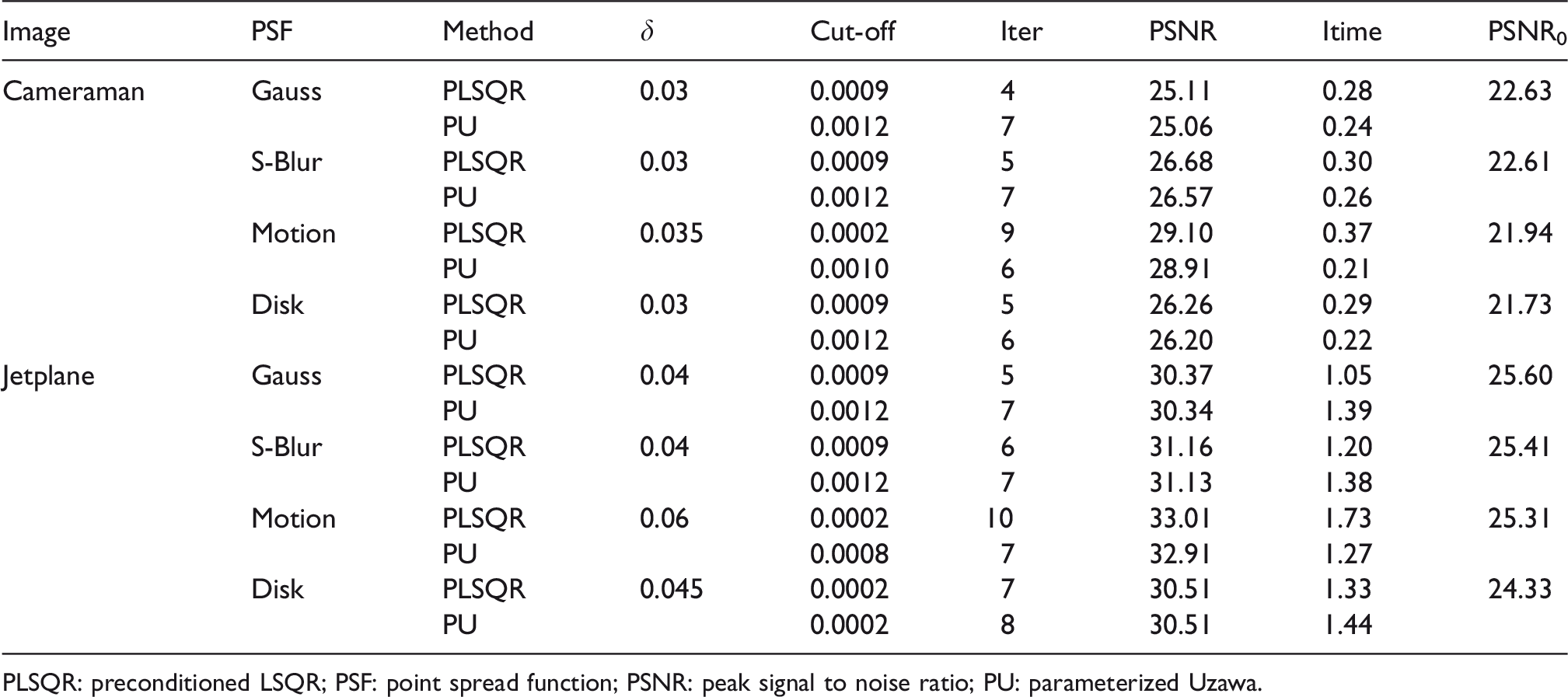
Numerical results for Case 1 of Tikhonov regularization problem.

Image	PSF	Method	δ	Cut-off	Iter	PSNR	Itime	PSNR0
Cameraman	Gauss	PLSQR	0.02	0.0009	2	25.25	0.20	22.63
		PU		0.0012	2	25.21	0.15
	S-Blur	PLSQR	0.02	0.0009	4	26.68	0.25	22.61
		PU		0.0012	2	26.67	0.15
	Motion	PLSQR	0.02	0.0002	6	29.34	0.29	21.94
		PU		0.0012	3	29.09	0.16
	Disk	PLSQR	0.02	0.0012	4	26.52	0.25	21.73
		PU		0.0004	2	26.52	0.15
Jetplane	Gauss	PLSQR	0.03	0.0012	2	30.43	0.63	25.60
		PU		0.0012	2	30.43	0.83
	S-Blur	PLSQR	0.03	0.0012	4	31.32	0.88	25.41
		PU		0.0012	2	31.31	0.83
	Motion	PLSQR	0.03	0.0009	5	33.58	1.02	25.31
		PU		0.0012	3	33.42	0.85
	Disk	PLSQR	0.03	0.0009	2	30.90	0.63	24.33
		PU		0.0010	2	30.88	0.81

PLSQR: preconditioned LSQR; PSF: point spread function; PSNR: peak signal to noise ratio; PU: parameterized Uzawa.

Table 2.

Numerical results for Case 2 of Tikhonov regularization problem.

Image	PSF	Method	δ	Cut-off	Iter	PSNR	Itime	PSNR0
Cameraman	Gauss	PLSQR	0.03	0.0009	4	25.11	0.28	22.63
		PU		0.0012	7	25.06	0.24
	S-Blur	PLSQR	0.03	0.0009	5	26.68	0.30	22.61
		PU		0.0012	7	26.57	0.26
	Motion	PLSQR	0.035	0.0002	9	29.10	0.37	21.94
		PU		0.0010	6	28.91	0.21
	Disk	PLSQR	0.03	0.0009	5	26.26	0.29	21.73
		PU		0.0012	6	26.20	0.22
Jetplane	Gauss	PLSQR	0.04	0.0009	5	30.37	1.05	25.60
		PU		0.0012	7	30.34	1.39
	S-Blur	PLSQR	0.04	0.0009	6	31.16	1.20	25.41
		PU		0.0012	7	31.13	1.38
	Motion	PLSQR	0.06	0.0002	10	33.01	1.73	25.31
		PU		0.0008	7	32.91	1.27
	Disk	PLSQR	0.045	0.0002	7	30.51	1.33	24.33
		PU		0.0002	8	30.51	1.44

PLSQR: preconditioned LSQR; PSF: point spread function; PSNR: peak signal to noise ratio; PU: parameterized Uzawa.

Table 3.

Numerical results for Case 3 of Tikhonov regularization problem.

Image	PSF	Method	δ	Cut-off	Iter	PSNR	Itime	PSNR0
Cameraman	Gauss	PLSQR	0.02	0.0009	2	25.20	0.22	22.63
		PU		0.0012	5	25.15	0.22
	S-Blur	PLSQR	0.02	0.0009	4	26.62	0.28	22.61
		PU		0.0012	5	26.65	0.22
	Motion	PLSQR	0.02	0.0002	6	29.19	0.32	21.94
		PU		0.0012	5	29.02	0.21
	Disk	PLSQR	0.025	0.0012	4	26.42	0.29	21.73
		PU		0.0010	5	26.28	0.22
Jetplane	Gauss	PLSQR	0.03	0.0009	2	30.38	0.63	25.60
		PU		0.0012	5	30.38	1.54
	S-Blur	PLSQR	0.03	0.0009	4	31.22	0.93	25.41
		PU		0.0012	5	31.22	1.51
	Motion	PLSQR	0.05	0.0009	5	33.58	1.04	25.31
		PU		0.0012	5	33.41	1.36
	Disk	PLSQR	0.04	0.0009	3	30.81	0.78	24.33
		PU		0.0012	5	30.72	1.54

PLSQR: preconditioned LSQR; PSF: point spread function; PSNR: peak signal to noise ratio; PU: parameterized Uzawa.

Table 4.

Numerical results for Case 1 of L1-norm regularization problem.

Image	PSF	Method	λ	μ	Cut-off	Iter	PSNR	Itime	PSNR0
Cameraman	Gauss	PLSQR	0.01	0.01	0.0009	14	25.22	1.19	22.63
		PU			0.0012	14	25.22	1.21
	S-Blur	PLSQR	0.01	0.01	0.0009	21	26.89	2.17	22.61
		PU			0.0012	21	26.89	1.83
	Motion	PLSQR	0.005	0.02	0.0009	18	30.74	2.71	21.94
		PU			0.0012	18	30.60	1.83
	Disk	PLSQR	0.007	0.014	0.0009	19	26.98	1.59	21.73
		PU			0.0012	19	26.98	1.41
Jetplane	Gauss	PLSQR	0.01	0.01	0.0009	8	30.53	3.34	25.60
		PU			0.0012	8	30.53	2.67
	S-Blur	PLSQR	0.01	0.01	0.0009	11	31.71	7.26	25.41
		PU			0.0012	11	31.71	4.33
	Motion	PLSQR	0.005	0.02	0.0009	9	34.61	7.24	25.31
		PU			0.0012	9	34.59	4.40
	Disk	PLSQR	0.007	0.014	0.0009	11	31.78	4.57	24.33
		PU			0.0012	11	31.78	3.40

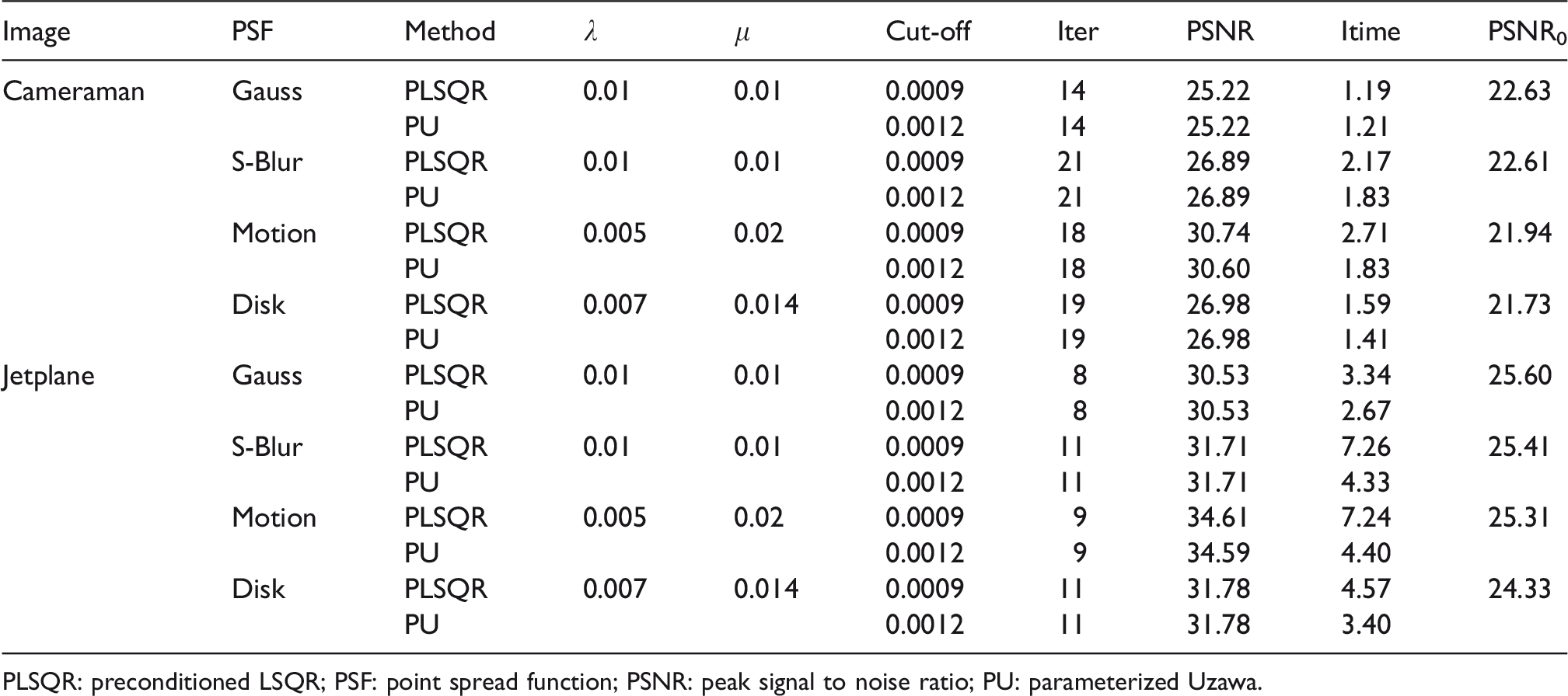
PLSQR: preconditioned LSQR; PSF: point spread function; PSNR: peak signal to noise ratio; PU: parameterized Uzawa.

Table 5.

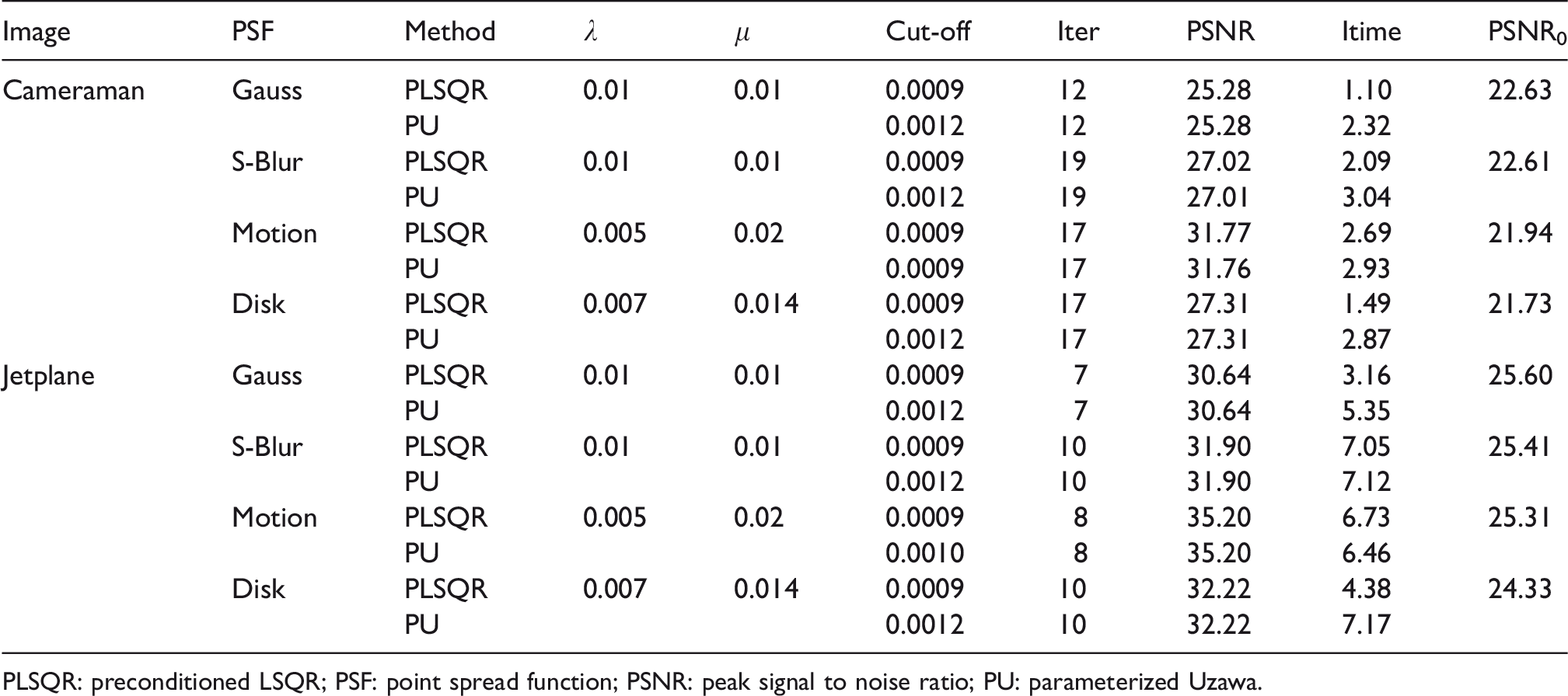
Numerical results for Case 2 of L1-norm regularization problem.

Image	PSF	Method	λ	μ	Cut-off	Iter	PSNR	Itime	PSNR0
Cameraman	Gauss	PLSQR	0.02	0.02	0.0009	18	25.52	4.38	22.63
		PU			0.0012	18	25.52	4.38
	S-Blur	PLSQR	0.02	0.02	0.0009	22	27.39	5.37	22.61
		PU			0.0012	22	27.39	5.25
	Motion	PLSQR	0.02	0.05	0.0009	20	32.13	6.73	21.94
		PU			0.0009	20	32.13	4.98
	Disk	PLSQR	0.02	0.03	0.0009	23	27.72	7.20	21.73
		PU			0.0012	23	27.72	6.42
Jetplane	Gauss	PLSQR	0.02	0.02	0.0009	10	30.84	13.3	25.60
		PU			0.0012	10	30.84	12.7
	S-Blur	PLSQR	0.02	0.02	0.0009	12	32.15	16.1	25.41
		PU			0.0012	12	32.15	15.2
	Motion	PLSQR	0.02	0.05	0.0009	10	35.18	18.7	25.31
		PU			0.0009	10	35.18	13.5
	Disk	PLSQR	0.02	0.03	0.0009	13	32.34	22.4	24.33
		PU			0.0012	13	32.34	19.7

PLSQR: preconditioned LSQR; PSF: point spread function; PSNR: peak signal to noise ratio; PU: parameterized Uzawa.

Table 6.

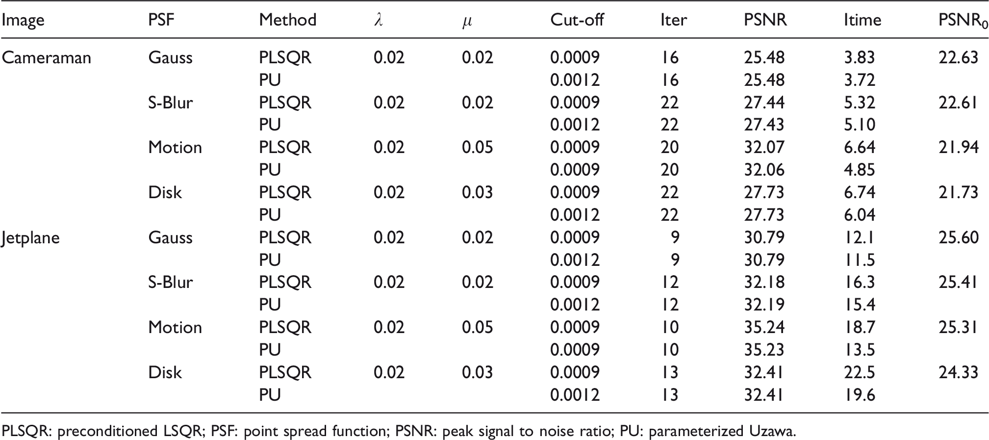
Numerical results for Case 3 of L1-norm regularization problem.

Image	PSF	Method	λ	μ	Cut-off	Iter	PSNR	Itime	PSNR0
Cameraman	Gauss	PLSQR	0.01	0.01	0.0009	12	25.28	1.10	22.63
		PU			0.0012	12	25.28	2.32
	S-Blur	PLSQR	0.01	0.01	0.0009	19	27.02	2.09	22.61
		PU			0.0012	19	27.01	3.04
	Motion	PLSQR	0.005	0.02	0.0009	17	31.77	2.69	21.94
		PU			0.0009	17	31.76	2.93
	Disk	PLSQR	0.007	0.014	0.0009	17	27.31	1.49	21.73
		PU			0.0012	17	27.31	2.87
Jetplane	Gauss	PLSQR	0.01	0.01	0.0009	7	30.64	3.16	25.60
		PU			0.0012	7	30.64	5.35
	S-Blur	PLSQR	0.01	0.01	0.0009	10	31.90	7.05	25.41
		PU			0.0012	10	31.90	7.12
	Motion	PLSQR	0.005	0.02	0.0009	8	35.20	6.73	25.31
		PU			0.0010	8	35.20	6.46
	Disk	PLSQR	0.007	0.014	0.0009	10	32.22	4.38	24.33
		PU			0.0012	10	32.22	7.17

PLSQR: preconditioned LSQR; PSF: point spread function; PSNR: peak signal to noise ratio; PU: parameterized Uzawa.

Table 7.

Numerical results of Algorithm 5 for TV regularization problem (3).

Image	PSF	Method	λ	μ	Cut-off	Iter	PSNR	Itime	PSNR0
Cameraman	Gauss	PLSQR	0.02	0.02	0.0009	16	25.48	3.83	22.63
		PU			0.0012	16	25.48	3.72
	S-Blur	PLSQR	0.02	0.02	0.0009	22	27.44	5.32	22.61
		PU			0.0012	22	27.43	5.10
	Motion	PLSQR	0.02	0.05	0.0009	20	32.07	6.64	21.94
		PU			0.0009	20	32.06	4.85
	Disk	PLSQR	0.02	0.03	0.0009	22	27.73	6.74	21.73
		PU			0.0012	22	27.73	6.04
Jetplane	Gauss	PLSQR	0.02	0.02	0.0009	9	30.79	12.1	25.60
		PU			0.0012	9	30.79	11.5
	S-Blur	PLSQR	0.02	0.02	0.0009	12	32.18	16.3	25.41
		PU			0.0012	12	32.19	15.4
	Motion	PLSQR	0.02	0.05	0.0009	10	35.24	18.7	25.31
		PU			0.0009	10	35.23	13.5
	Disk	PLSQR	0.02	0.03	0.0009	13	32.41	22.5	24.33
		PU			0.0012	13	32.41	19.6

PLSQR: preconditioned LSQR; PSF: point spread function; PSNR: peak signal to noise ratio; PU: parameterized Uzawa.

Table 8.

Numerical results of Algorithm 5 for TV regularization problem (4).

Image	PSF	Method	λ	μ	Cut-off	Iter	PSNR	Itime	PSNR0
Cameraman	Gauss	PLSQR	0.02	0.02	0.0	16	25.48	4.04	22.63
		PU			0.0	16	25.48	4.10
	S-Blur	PLSQR	0.02	0.02	0.0	21	27.40	5.34	22.61
		PU			0.0	22	27.43	5.38
	Motion	PLSQR	0.02	0.05	0.0	20	32.07	7.01	21.94
		PU			0.0	20	32.06	5.12
	Disk	PLSQR	0.02	0.03	0.0	22	27.73	7.10	21.73
		PU			0.0	22	27.73	6.33
Jetplane	Gauss	PLSQR	0.02	0.02	0.0	9	30.79	12.4	25.60
		PU			0.0	9	30.79	11.8
	S-Blur	PLSQR	0.02	0.02	0.0	12	32.18	16.7	25.41
		PU			0.0	12	32.19	15.5
	Motion	PLSQR	0.02	0.05	0.0	10	35.23	19.2	25.31
		PU			0.0	10	35.23	13.8
	Disk	PLSQR	0.02	0.03	0.0	13	32.41	23.1	24.33
		PU			0.0	13	32.41	20.1

PLSQR: preconditioned LSQR; PSF: point spread function; PSNR: peak signal to noise ratio; PU: parameterized Uzawa.

Table 9.

Numerical results of Algorithm 6 for TV regularization problem (4).

Image	PSF	Method	λ	μ	Cut-off	Iter	PSNR	Itime	PSNR0
Cameraman	Gauss	PLSQR	0.0004	0.04	0.0	70	25.37	5.64	22.63
		PU			0.0	70	25.37	4.17
	S-Blur	PLSQR	0.0004	0.01	0.0	29	27.00	3.04	22.61
		PU			0.0	29	27.00	2.40
	Motion	PLSQR	0.0004	0.05	0.0	53	30.78	6.56	21.94
		PU			0.0	53	30.79	3.77
	Disk	PLSQR	0.0004	0.02	0.0	38	27.03	3.03	21.73
		PU			0.0	38	27.03	2.37
Jetplane	Gauss	PLSQR	0.0004	0.02	0.0	51	30.81	20.7	25.60
		PU			0.0	51	30.81	12.8
	S-Blur	PLSQR	0.0004	0.02	0.0	45	31.91	29.1	25.41
		PU			0.0	45	31.92	14.8
	Motion	PLSQR	0.0004	0.07	0.0	65	34.40	42.0	25.31
		PU			0.0	65	34.41	20.8
	Disk	PLSQR	0.0004	0.04	0.0	56	31.49	22.9	24.33
		PU			0.0	56	31.49	13.9

PLSQR: preconditioned LSQR; PSF: point spread function; PSNR: peak signal to noise ratio; PU: parameterized Uzawa.

The preconditioners Q for the PU method are chosen as was described in the “Relaxation iterative methods for Tikhonov regularization problem” section, i.e. Q = C^TΣ C, and the preconditioners $\tilde{Q}$ for the PLSQR method are chosen as $\tilde{Q}=Q^{1/2}=C^T{\Sigma }^{1/2}C$ , where C is the two-dimensional discrete cosine transformation matrix described in the “Relaxation iterative methods for Tikhonov regularization problem” section.

All numerical tests have been performed using Matlab R2017b on a personal computer equipped with Intel Core i5-4570 3.2 GHz CPU and 8 GB RAM. For numerical experiments, we have used four types of PSFs which are Gaussian blur, S-blur, Motion blur, and Disk blur of size 9 × 9. The PSF array P for Gaussian blur of size 9 × 9 is generated by the Matlab function $\mathit{fspecial}(\prime \mathit{gaussian}\prime ,[9,9],2)$ . The PSF array P for S-blur of size 9 × 9 is given by

$$\begin{array}{l}K={\left(123454\frac{5}{2}\frac{3}{2}\frac{1}{2}\right)}^T\otimes \left(\frac{1}{4}\frac{1}{3}\frac{1}{2}\frac{3}{4}1\frac{3}{4}\frac{1}{2}\frac{1}{4}\frac{1}{8}\right)\\ P=\frac{K}{{\displaystyle {\sum }_{i,j=1}^9{k}_{\mathit{ij}}}}\end{array}$$

where k_ij denotes the (i, j)-component of K. The PSF array P for Disk blur of size 9 × 9 is generated by the Matlab function $\mathit{fspecial}(\prime \mathit{disk}\prime ,4)$ , and the PSF array P for Motion blur of size 9 × 9 is generated by the Matlab function

$$P=\mathit{zeros}\left(9\right);P\left(4:6,:\right)=\mathit{fspecial}\left(\prime \mathit{motion}\prime ,9,1\right)$$

The blurred and noisy image b is generated by

$$b=Ax+\mathit{vec}(E)$$

where A stands for the blurring matrix which can be generated by the original PSF array P according to the reflexive boundary condition, and the noise E is a Gaussian white noise with mean 0 and standard deviation 0.95 which can be generated using Matlab function randn. That is

$$E=0.95\times \mathit{randn}(m,n)$$

where (m, n) denotes the size of the true image X = array(x). A restored image G is measured by the peak signal to noise ratio (PSNR) which is defined by

$$\text{PSNR}=10{\text{log}}_{10}\left(\frac{{\max }_{i,j}|x_{\mathit{ij}}{|}^2·m·n}{{\Vert X-G\Vert }_F^2}\right)$$

where X = (x_ij) represents the true image and ${\Vert ·\Vert }_F$ denotes the Frobenius norm.

We have used two test images called Cameraman and Jetplane for numerical experiments (see Figure 1). The pixel size of Cameraman image is 256 × 256, and the pixel size of Jetplane image is 512 × 512. The blurring matrix A whose size is large is not constructed since its construction is very time-consuming and matrix-vector multiplication with A can be performed without constructing A (see Hankey and Nagy ¹ for details).

Figure 1.

(a, b): Cameraman images, (c, d): Jetplane images, (b, d): Noisy images blurred by Motion Blur. (a) True image, (b) blurred and noisy image, (c) true image, and (d) blurred and noisy image.

In Tables 1 to 9, “Cut-Off” represents the Cut-Off values that are used for constructing the preconditioners Q and $\tilde{Q}$ , “PSNR” represents the PSNR values for the restored images, PSNR₀ represents the PSNR value for the blurred and noisy image, “Itime” denotes the elapsed CPU time in seconds required for all iteration steps which include computational step of finding preconditioners and computational step of finding near optimal relaxation parameters ω and τ, “Iter” denotes the number of iterations of Algorithms 1, 3, 5, and 6 satisfying the stopping criterions, and “δ, λ, μ” denote near optimal regularization parameters which are chosen by numerical tries. The parameter α for TV regularization problem (4) is set to 10⁻⁶ for Algorithm 5 and 2 × 10⁻³ for Algorithm 6, and the parameter κ for Algorithm 6 is set to 10⁻⁶.

Numerical results for Tikhonov regularization problem (1) are provided in Tables 1 to 3 and Figure 2, and numerical results for L1-norm and TV regularization problems (2) to (4) are provided in Tables 4 to 9 and Figures 3 and 4. As can be seen in Tables 1 to 9 and Figures 2 to 4, deblurring algorithms using PU method restore the true image as well as those using PLSQR method except for the Motion blur of Tikhonov regularization problem for which PLSQR restores the true image a little bit better than PU. As may be expected, Split Bregman methods for L1-norm and TV regularization problems (2) to (4) and fixed point method for TV regularization problem (4) restore the true image better than deblurring algorithms for Tikhonov regularization problem.

Figure 2.

Restored images by Tikhonov regularization problem for Motion blur ((a, b, c): restored images by PLSQR for three cases of D, (d, e, f): restored images by PU for three Cases of D). (a) Case 1 (PSNR = 29.34), (b) Case 2 (PSNR = 29.10), (c) Case 3 (PSNR = 29.19), (d) Case 1 (PSNR = 29.09), (e) Case 2 (PSNR = 28.91), and (f) Case 3 (PSNR = 29.02).

Figure 3.

Restored images by L1-norm regularization problem and TV regularization problem (3) for Motion blur ((a, b, c): restored images by PLSQR for two cases of D and TV, (d, e, f): restored images by PU for two cases of D and TV). (a) Case 1 (PSNR = 34.61), (b) Case 3 (PSNR = 35.20), (c) TV (PSNR = 35.24), (d) Case 1 (PSNR = 34.59), (e) Case 3 (PSNR = 35.20), and (f) TV (PSNR = 35.23).

Figure 4.

Restored images by TV regularization problem (4) for Motion blur ((a, c): restored images by Split Bregman method, (b, d): restored images by fixed point method, (a, b): restored images by PLSQR, (c, d): restored images by PU). (a) TV (PSNR = 32.07), (b) TV (PSNR = 30.78), (c) TV (PSNR = 32.06), and (d) TV (PSNR = 30.79).

For Tikhonov regularization problem, deblurring algorithms using PU have less execution time than those using PLSQR for small size of Cameraman image, while deblurring algorithms using PU have more execution time than those using PLSQR for large size of Jetplane image (see Tables 1 to 3). The reason for this is that computational step of finding near optimal relaxation parameters ω and τ of the PU method requires a lot of CPU time for large size of images.

For L1-norm and TV regularization problems, Split Bregman methods using PU have less execution time than those using PLSQR except for Case 3 of L1-norm regularization problem (see Tables 4 to 8). For Case 3 of L1-norm regularization problem, Split Bregman methods using PU have more execution time than those using PLSQR. This is because convergence rate of PU method is slower than that of PLSQR method for every iteration of Split Bregman method. For Split Bregman method, near optimal relaxation parameters ω and τ of the PU method are computed only once at the first iteration, so computing time for finding near optimal relaxation parameters ω and τ is negligible since it is small as compared with the total computing time of Split Bregman method.

Algorithm 5 for TV regularization problem (4) performs almost as well as that for TV regularization problem (3) (see Tables 7 and 8). Problem (4) has one additional parameter α, but it has some advantages that Cut-Off value is not required and one value of α = 10⁻⁶ performs well for all test problems. On the other hand, problem (3) requires a Cut-Off value which varies depending upon test problems to be used. In this respect, TV regularization problem (4) may have a preference over problem (3).

Split Bregman method for problem (4) (i.e. Algorithm 5) restores the true image better and has faster convergence rate than the fixed point method for problem (4) (i.e. Algorithm 6) (see Tables 8 and 9). Since the fixed point method has slow convergence rate and computational amount of PU per iteration is smaller than that of PLSQR, Algorithm 6 using PU has much less execution time than that using PLSQR (see Table 9).

Conclusions

In this paper, we have studied efficient applications of relaxation iterative methods to four types of image deblurring problems which are Tikhonov, L1-norm, and TV regularization problems. To this end, we proposed how to find good preconditioners and near optimal relaxation parameters which provide fast convergence rate and efficient computation for relaxation iterative methods. Numerical experiments show that these techniques work well for deblurring algorithms using relaxation iterative methods.

For Tikhonov regularization problem, deblurring algorithms using PU have less execution time than those using PLSQR for small size of Cameraman image, while deblurring algorithms using PU have more execution time than those using PLSQR for large size of Jetplane image since finding near optimal relaxation parameters ω and τ of the PU method requires a lot of CPU time for large size of images.

For Split Bregman and fixed point methods solving L1-norm and TV regularization problems, near optimal relaxation parameters ω and τ of PU are computed only once at the first iteration, so computing time for finding the near optimal parameters is negligible since it is small as compared with the total computing time of Split Bregman and fixed point methods. Hence, Split Bregman and fixed point methods using PU have less execution time than those using PLSQR. In particular, the fixed point method using PU has much less execution time than that using PLSQR since the fixed point method has slow convergence rate. Overall, Split Bregman and fixed point methods using PU with near optimal relaxation parameters perform quite well in terms of both PSNR values and execution time as compared with PLSQR.

Split Bregman method for TV regularization problem (4) performs almost as well as that for TV regularization problem (3). Even if problem (4) has one additional parameter α, it does not require Cut-Off and one value of α = 10⁻⁶ performs well for all test problems. However, problem (3) requires a Cut-Off value which should be well chosen appropriately for each test problem. In this regard, TV regularization problem (4) may have a preference over TV regularization problem (3).