Jointly Linear Embedding via L 2,1 -Norm for Dimensionality Reduction

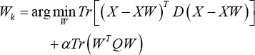
Abstract

In this study, we present a novel dimensionality reduction method called Jointly Linear Embedding (JLE). Unlike previous methods such as Neighborhood Preserving Embedding (NPE), in which local neighborhood information is preserved during the dimensionality reduction procedure, JLE aims to preserve the sparse reconstructive relationship of the original data by taking the merits of jointly sparse learning based on L_2,1-norm. In the framework of JLE, the sparse weight matrix can reflect the intrinsic geometric structures of the original data and inherit the ability of discriminant analysis. By solving the L_2,1-norm regularized objective function, the optimal projections, which are invariant to rotations and robust to outliers, can be obtained by JLE. Extensive experiments on visual recognition and fabric defect classification datasets demonstrate the superiority of the proposed L_2,1-norm regularized learning method compared with the state-of-the-art methods.

Introduction

Data with high dimensions exist in many real-world applications, such as content-based image retrieval, visual recognition, feature clustering, and multi view data handling,^1–4 which raises great challenges for human society. Therefore, it is important to perform dimensionality reduction on the data by effectively exploiting the underlying structure information and the discriminative information.

The goal of dimensionality reduction is to map the high-dimensional samples to a low dimensional space, while preserving the structure properties among the data points. Up to now, researchers have developed many linear and nonlinear dimensionality reduction methods. Principal Component Analysis (PCA)^5–8 and Linear Discriminant Analysis (LDA)^9–11 are two classical linear dimensionality reduction methods. The idea of PCA is to find a set of optimal projections by maximizing the variance of the original data. To explore the projections with discriminant power, LDA attempts to maximize the ratio of between-class scatter and within-class scatter. Besides the linear analysis methods, several nonlinear techniques also have been proposed to discover the nonlinear structure of the manifold. The representative methods include Laplacian Eigenmap, ¹² Locally Linear Embedding, ¹³ Isomap, ¹⁴ Maximum Variance Unfolding (MVU), ¹⁵ Stochastic Neighbor Embedding (SNE), ¹⁶ and t-Distributed Stochastic Neighbor Embedding (t-SNE) ¹⁷ These nonlinear methods can discover nonlinear structure of the data to learn a low-dimensional representation. Even though nonlinear techniques are effective under certain conditions, they are not competitive in efficiency. Moreover, these methods are normally not easy to configure in real-world applications. Therefore, the manifold-learning-based linear dimensionality reduction have been a hot research topic since the past decade. The well-known techniques include Locality Preserving Projection (LPP) ¹⁸ and Neighborhood Preserving Embedding (NPE). ¹⁹ LPP is a linear approximation of the nonlinear Laplacian Eigen-maps, which seek to find the projections to optimally preserve the nearest neighborhood relationship among the data points.^20–22 Unlike LPP, NPE is a linear approximation of Locality Linear Embedding (LLE), ¹³ which seeks for the projections such that the local reconstructive relationship can be preserved in low-dimensional space.

In recent years, sparse representation or sparse regression methods were popularized in the field of visual recognition.^26–28 Based on the concept of sparse regression, Sparse PCA (SPCA) ²⁹ extended the classical principle component analysis by using the L₁-norm Elastic Net regression. It was verified that the sparsity was an effective way for signal identification.^23–25 With the merits of sparsity, the recently proposed Sparsity Preserving Projections (SPP) ³⁰ introduced the L₁-norm regularization to effectively select the discriminative features and avoid the over-fitting problem. SPP can preserve the sparsity reconstructive relationship of the data. However, it neglects the dependence between the representations of different samples. To learn discriminative features from 2D image matrix directly, Lai et al. ³¹ designed a hybrid scheme by combining L₁-norm and L₂-norm regressions together to find the 2D-based image matrix projections.

However, both conventional dimensionality methods (LPP and NPE) take the L₂-norm for measurement, which make these approaches vulnerable to outliers. Even though the recently proposed SPP adopts the L₁-norm and L₂-norm for measurement and adjacent graph learning, it still lacks the well interpretation for subspace learning.

Recently, the L_2,1-norm-based feature selection methods received considerable attention.^32–43 Nie et al. ³⁴ offered an effective approach for solving the joint L_2,1-norm based minimization problem and the convergence proof was given. Nie et al. also leveraged joint L_2,1-norm minimization on both loss function and regularization for feature selection. In another work, Li et al. ⁴¹ proposed an unsupervised learning algorithm (Nonnegative Discriminant Feature Selection), in which the L_2,1-norm minimization constraint was added into the objective function for guaranteeing that the projection matrix is sparse in rows. Hou et al. ⁴² also introduced a novel unsupervised feature selection approach, via jointly Embedding Learning and Sparse Regression, in which the L_2,1-norm regularization is added for learning a sparse feature ranking matrix. To achieve the goal of unsupervised feature selection, Yang et al. ⁴³ incorporated discriminative analysis and L_2,1-norm minimization into a joint subspace learning framework. Recent studies^44,45 showed that low-rank learning is effective in dimensionality reduction and feature extraction.^46,47 However, the noises had great influence on low-rank feature learning. To solve this problem, Lu et al. ⁴⁸ and Wen et al. ⁴⁹ proposed to impose the L_2,1-norm on the regularization terms of the optimization model, which shows competitive performance of the L_2,1-norm in low-rank sub-space learning. The L_2,1-norm-based sparse weight matrix is row-wise consistent, while the L₁-norm based matrix is not. ³⁴ In the consistent sparsity weight matrix, all the elements in certain rows that have nothing to do with sub-space learning trend to be zero, which avoids the influence of outliers (corresponding to the rows with zero elements) on the reconstruction task. However, in the “conventional sparsity” weight matrix, which is exploited by L₁-norm-based optimization, zero elements randomly appear on the learned matrix, which makes it hard to decide the optimal features or data points (items in row) for further processing. Besides, the L₂-norm, which is sensitive to outliers, is still dominant in the objective function of the conventional sparse regression methods. Therefore, the L_2,1-norm based weight matrix is more robust than the L₁-norm based weight matrix due to its following properties.

1. 1)

The optimization with L_2,1-norm regularization is able to perform jointly sparse learning.

2)

The matrix learned from the L_2,1-norm-based model has well interpretation. Specifically, the nonzero vectors on the rows of the learned matrix indicate the valuable data or features for representation. The zero vectors on the rows of the learned matrix indicate the useless part or feature of the original data.

3)

The L_2,1-norm-based model is robust to outliers.

4)

The L_2,1-norm-based model has a close-form iterative solution.

Zhao et al. ³⁵ used spectral regression with L_2,1-norm constraint to jointly evaluate the features. It was reported that their method can effectively remove the redundant features. Ren et al. ³⁶ exploited L_2,1-norm minimization of both loss function and regularization for classification. All of these methods^33–40 used the same method presented in another reference ³⁴ to solve the joint L_2,1-norm-based loss function and regularization minimization problem.

Motivated by jointly sparse learning, which is robust to outliers, in this study, the L_2,1-norm is introduced to two crucial steps (weight matrix learning and projection matrix learning) for jointly linear embedding (JLE) to perform robust dimensionality reduction. As mentioned above, the L_2,1-norm-based method is robust to outliers as compared with the L₂-norm-based method. Therefore, unlike conventional dimensionality reduction methods, such as LPP and NPE that use L₂-norm for measurement during the weight matrix optimization step, JLE acquires the adjacent weights of the data points via jointly sparse learning with the merits of the L_2,1-norm. Thus the linear embedding based on the measurement of the L_2,1-norm is integrated into the second phase optimization framework to learn optimal projections for obtaining the sparse reconstructive relationship. Therefore, in this work, we propose a novel linear embedding method, which solves the joint L_2,1-norm-based minimization problem with its convergence proof given.

The contributions of this paper are summarized as follows:

1. 1)

By exploiting the L_2,1-norm-based weight matrix learning, the proposed method obtains the weight matrix with “consistent sparsity.” This weight matrix can indicate data points that play an important role in the reconstruction task. Compared with LPP, NPE, and SPP, the proposed L_2,1-norm-based weight matrix learning is more robust to outliers and the obtained weight matrix can reflect the intrinsic geometric structures of the original data.

2)

JLE is able to take the merits of L_2,1-norm to learn the optimal projections that preserve the sparse reconstructive relationship among the data points. Similarly, the L_2,1-norm makes JLE invariant to rotations and robust to outliers.

3)

A new linear embedding dimensionality reduction framework with two phases optimization based on L_2,1-norm is proposed. We have designed an effectively iterative method to solve the proposed model with the convergence proof provided. Moreover, a quantity of experiments with outlier handling is designed to verify the competitiveness of the proposed method.

The reminder of this paper is organized as follows. The notations of the proposed method and the related works are introduced, and an L_2,1-norm-based jointly linear embedding algorithm with its convergence proof is presented. To evaluate the effectiveness of the proposed method compared with state-of-the-art methods, a number of experiments are performed on the public datasets, followed by the conclusion.

Related Works

In this section, we give some definitions and notations, and then briefly review the closely related methods NPE ¹⁹ and SPP. ³⁰

Notations and Definitions

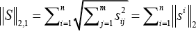
We first give some notations and definitions of different norms. The matrix and vectors are represented with uppercase letters and lowercase letters, respectively. For matrix S = (s _ij ), its i-th row and j-th column are denoted by s ⁱ and s _j , with superscript and subscript, respectively.

The L₂-norm of the vector v ∈ ℝ ⁿ is defined as $\Vert v{\Vert }_2=\sqrt{{\displaystyle {\sum }_{i=1}^n{v}_i^2}}$ , which is defined as the square root of the summation of the square value of the elements. The Frobenius norm of the matrix S ∈ ℝ ^nxm is defined in Eq. 1.

$$\Vert S{\Vert }_F=\sqrt{{\displaystyle {\sum }_{i=1}^n{\displaystyle {\sum }_{j=1}^m{s}_{ij}^2}}}=\sqrt{{{\displaystyle {\sum }_{i=1}^n\Vert s^i\Vert }}_2^2}$$

Eq. 1

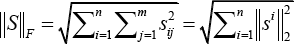
and the L_2,1-norm ³⁴ of the matrix S ∈ ℝ^nxm is defined in Eq. 2.

$$\Vert S{\Vert }_{2,1}={\displaystyle \sum _{i=1}^n\sqrt{{\displaystyle \sum _{j=1}^m{s}_{ij}^2}}}={\displaystyle \sum _{i=1}^n\Vert {\Vert }^i}{\Vert }_2$$

Eq. 2

We consider a set of n sample images X = [x₁ x₂ · · · x _n ]∈ ℝ^rxn taken from an r-dimensional image space. Due to the high dimensionality, it is inefficient to directly apply visual algorithms on the raw data. Therefore, it is of vital importance to perform dimensionality reduction on the original data. We design a linear transformation, which maps the original r-dimensional images space into a d-dimensional feature space. Let A ∈ ℝ ^rxd be the linear transformation. The method of dimensionality reduction here projects each image x., an r x 1 dimensional vector, onto a low-dimensional space by the transformation in Eq. 3.

$$y_i=A^T{x}_i$$

Eq. 3

NPE

NPE ¹⁹ is a subspace learning algorithm, which aims at preserving the local neighborhood structure of the data manifold. In the NPE algorithm, the first step constructs an adjacent graph. Then, the second step computes the weights on the edges by minimizing the objective function, as shown in Eq. 4.

$${\min }_W{\displaystyle \sum _i{\Vert x_i-{\displaystyle \sum _{j=1,2,\cdots ,n}{w}_{ij}}{x}_j\Vert }^2}$$

Eq. 4

with constraints in Eq. 5.

$${\displaystyle \sum _j{w}_{ij}}=1,j=1,2,\cdots ,n$$

Eq. 5

The third step computes the linear projections a by solving the generalized eigenvector problem using Eq. 6.

$$XM{X}^{T}a=\lambda X{X}^{T}a$$

Eq. 6

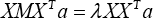
where λ is a scale factor, M is defined in Eq. 7.

$$M=(I-W){(I-W)}^T$$

Eq. 7

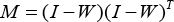
I is the unit matrix and A = [a₁ a₂ · · · a _d ].

SPP

Both SPP ³⁰ and NPE are closely related to LLE. ¹³ In fact, NPE is a directly linear approximation of LLE, while SPP constructs the “affinity” weight matrix in a completely different manner compared with LLE. In particular, SPP constructs the weight matrix using all the training samples (with sparsity constraints) instead of k nearest neighbors.

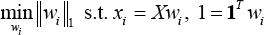
For SPP, each sample is reconstructed by the related samples whose number is as small as possible. They seek a sparse reconstructive weight vector w _i ∈ ℝ ^rx1 for each x _i . through a modified L₁-norm optimization problem (Eq. 8), where X = [x₁ ··· x _j ··· x _n ] ∈ ℝ^mxn, each element of w _i . represents the contribution (reconstructive weight) of x _j to reconstruct x _i .

$${\min }_{x_i}{\Vert w_i\Vert }_1\text{ s}.\text{t}.x_i=X{w}_i,1=1^T{w}_i$$

Eq. 8

Given a visual image x _i ^j from the j-th class, x _i ^j can be theoretically represented using the samples from the j-th class Thus we have Eq. 9.

$$x_i^j=0·x_1^1+\cdots +{\alpha }_{i,i-1}{x}_{i-1}^j+{\alpha }_{i,i+1}{x}_{i+1}^j+\cdots +0·x_r^n:$$

Eq. 9

where j = 1,2, ···, n. The weights vector

$$w_i={\left[\begin{array}{lllllll}0\hfill & \cdots \hfill & {\alpha }_{i,i-1}\hfill & 0\hfill & {\alpha }_{i,i+1}\hfill & \cdots \hfill & 0\hfill \end{array}\right]}^{\prime }$$

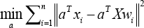
is sparse. Similar to LLE and NPE, SPP defines the objective function (Eq. 10) to seek the projections which best preserve the optimal weight vectors w _i . ³⁰

$${\min }_a{\displaystyle \sum _{i=1}^n{\Vert a^T{x}_i-a^{T}X{w}_i\Vert }^2}$$

Eq. 10

The optimal projection vectors a can be obtained by solving the generalized eigenvalue problem, as shown in Eq. 11.

$$X\left(W+W^T-W^{T}W\right)X^{T}a=\lambda X{X}^{T}a$$

Eq. 11

and the eigenvectors corresponding to the largest d eigenvalues span the optimal subspace.

Proposed Method

To perform jointly sparse learning and linear embedding, the L_2,1-norm was used in the phases of weight matrix learning and projection matrix learning under the dimensionality reduction framework. The proposed method is called Jointly Linear Embedding (JLE), which will be explored and elaborated in detail in this section. We not only show the model of L_2,1-norm-based jointly sparse learning and the model of L_2,1-norm-based jointly linear embedding learning, but also design effectively iterative methods to solve the proposed models with their convergence proof provided in theory.

Jointly Sparse Learning Based Weight Matrix Construction

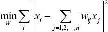
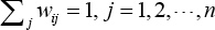
In image recognition, it is important to obtain the discriminant features for visual representation and recognition. Therefore, in this work, the latent intrinsic discriminative features were extracted from the visual images (e.g. faces images and fabric defect images) to improve the classification rate and enhance the robustness. Recent research^50,51 indicates that the performance of discriminative feature selection and recognition rate can be further improved by introducing the L_2,1-norm into the optimization problem. To take the merits of L_2,1-norm for jointly sparse learning, we integrate the L_2,1-norm into the weight matrix optimization model to obtain a robust sparse weight matrix for linear embedding. We expect that both sample representation and weight matrix could be robust to the outliers. To this end, the L_2,1-norm will be imposed on both dominant term and the regularization term to formulate the optimization problem using Eq. 12.

$${\min }_W\Vert X-XW{\Vert }_{2,1}+\alpha \Vert W{\Vert }_{2,1}$$

Eq. 12

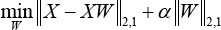
where W ∈ ℝ^nxn is the weight matrix and α is the regularization parameter. For a sample in X, the dominant term of Eq. 12 selects the closely related samples among X for linearly representing this sample. The number of selected samples should be as small as possible. This can be guaranteed by the L_2,1-norm that holds an effectiveness of jointly sparse learning. To fully achieve the functionality of jointly sparse learning, we impose the L_2,1-norm on the weight matrix as shown in the regularization term of Eq. 12, so that the weight matrix could be sparse in row, which shows good robustness to the outliers. The obtained sparse weight matrix is able to indicate the relation between the samples. Compared with the L₂-norm-based measurement in LLE, the proposed L_2,1-norm-based measurement is imposed on both dominant term and regularization term, which turns out to be more robust. When using the L_2,1-norm to do sample selection for reconstruction, the objective function in Eq. 12 can exclude the samples not closely related to the test sample in the robust regularized regression. It is obvious that the reconstructive property is decided by the data and the L_2,1-norm optimization algorithm, and not decided by the k nearest neighbor, which is quite different from classical locally linear reconstruction. Although solving the joint L_2,1-norm problem seems difficult, we show that this problem can be solved using a simple yet effective algorithm.

To optimize the robust joint L_2,1-norm minimization function in Eq. 13, we do not need to solve it using the method proposed in the literature. ³⁴ Instead, we can directly solve the optimization problem in pursuit of a close-form solution in each iteration.

Denote E = X - XW, where D ∈ ℝ^rxr and Q ∈ ℝ^nxn are diagonal matrices whose i-th diagonal elements are D _ii = 1/2 ||E ⁱ ||₂ and Q _ii = 1/2 W ⁱ ||₂, respectively. Then, Eq. 12 can be rewritten as Eq. 13.

$$\begin{array}{l}\hspace{0.17em}\hspace{0.17em}\hspace{0.17em}\hspace{0.17em}\underset{W}{\min }\Vert X-XW{\Vert }_{2,1}+\alpha \Vert W{\Vert }_{2,1}\\ =\underset{W}{\min }\mathrm{Tr}\left[{(X-XW)}^{T}D(X-XW)\right]+\alpha \mathrm{Tr}\left(W^{T}QW\right)\\ =\underset{W}{\min }\mathrm{Tr}\left[\left(X^T-W^T{X}^T\right)D(X-XW)\right]+\alpha \mathrm{Tr}\left(W^{T}QW\right)\\ =\underset{W}{\min }\mathrm{Tr}[X^{T}DX-X^{T}DXW-W^T{X}^{T}DX+W^T{X}^{T}DXW]+\alpha \mathrm{Tr}\left(W^{T}QW\right)\\ =\underset{W}{\min }\mathrm{Tr}\left[X^{T}DX-2X^{T}DXW+W^T{X}^{T}DXW\right]+\alpha \mathrm{Tr}\left(W^{T}QW\right)\end{array}$$

Eq. 13

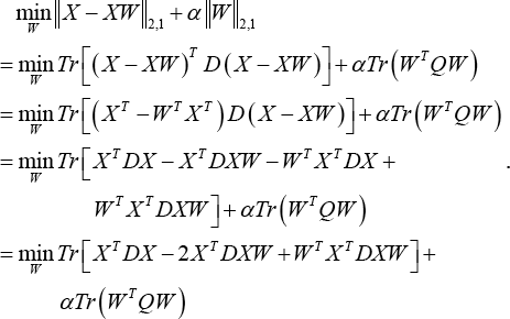
Define

$$L(W)=\mathrm{Tr}\left[X^{T}DX-2X^{T}DXW+W^T{X}^{T}DXW\right]\text{ +}\alpha \mathrm{Tr}\left(W^{T}QW\right)$$

Eq. 14

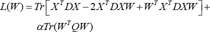
and taking the derivative of L(W) with respect to W to find the optimal value of the optimization problem. Then setting the obtained formula to zero, we have Eq. 15.

$$\frac{\partial L}{\partial W}=-2X^{T}DX+2X^{T}DXW+2\alpha QW=0$$

Eq. 15

Namely Eq. 16.

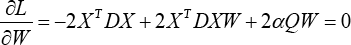
$$\left(X^{T}DX+\alpha Q\right)W=X^{T}DX$$

Eq. 16

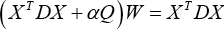
Therefore, the recursive formula of W is given in Eq. 17.

$$W={\left(X^{T}DX+\alpha Q\right)}^{-1}{X}^{T}DX$$

Eq. 17

Even though the variables D, Q, and W are all dependent on each other, the optimal values of the three matrices can be approximated and obtained via an iterative optimization algorithm. The proposed algorithm will fix the values of D and Q to compute W, and then fix W to update D and Q. The iteration does not stop until the convergence of the algorithm. The details of the iterative algorithm can be found in Algorithm 1.

Algorithm 1:

Solving the weight matrix

Input: Original data X ∈ ℝ rxn

1. Initialization: Set k = 0 and initialize the diagonal matrix D0 ∈ ℝ rxr , Q0 ∈ ℝ nxn as identity matrix.

2. Repeat:

3. Calculate the weight matrix Wk1+1 for Eq. 17 using current D0 and Q0 to obtain Wk+1 = (X T D0X + αQ0) X T D0X.

4. Update the diagonal matrices D and Q based on the current calculated Wk+1, which means that we should calculate the diagonal matrix Dk+1 and Qk+1, where the i-th diagonal elements are $1/2\Vert e_{k+1}^i\Vert$ and $1/2\Vert w_{k+1}^i\Vert$ , where Ek+1 = X - XWk+1, e i k+1 denotes the i-th row of the matrix Ek+1, and wk+1, denotes the i-th row of the matrix Wk+1.

5. Let k = k + 1.

6. Until convergence

Output: Weight matrix W

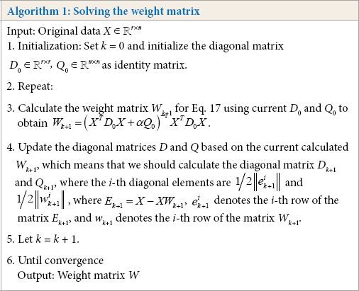
We show that Algorithm 1 converges, with the convergence proof presented below.

Lemma 1: When vectors w ⁱ _k , i = 1,2, ···, m are non-zero vectors, the inequality in Eq. 18 holds. ³⁴

$${\displaystyle \sum _i{\Vert w_{k+1}^i\Vert }_2}-{\displaystyle \sum _i\frac{{\Vert w_{k+1}^i\Vert }_2^2}{2{\Vert w_k^i\Vert }_2}}\le {\displaystyle \sum _i{\Vert w_k^i\Vert }_2}-{\displaystyle \sum _i\frac{{\Vert w_k^i\Vert }_2^2}{2{\Vert w_k^i\Vert }_2}}$$

Eq. 18

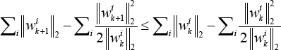
Proof: The proof of Lemma 1 can be found in the literature. ³⁴

Theorem 1: The iterative approach in Algorithm 1 monotonically decreases the objective function value of $\underset{W}{\min }\mathrm{Tr}\left|{(X-XW)}^{T}D(X-XW)\right|+\alpha \mathrm{Tr}\left(W^{T}QW\right)$ in each iteration.

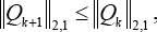
Proof: According to the definition of W _k in Algorithm 1, Eq. 19 can be formulated.

$$W_k=\arg \underset{W}{\min }\mathrm{Tr}\left[{(X-XW)}^{T}D(X-XW)\right]+\alpha \mathrm{Tr}\left(W^{T}QW\right)$$

Eq. 19

Thus, we have the expression in Eq. 20.

$${\displaystyle \sum _i\frac{{\Vert e_k^i\Vert }_2^2}{2{\Vert e_{k-1}^i\Vert }_2}}+\alpha {\displaystyle \sum _i\frac{{\Vert w_k^i\Vert }_2^2}{2{\Vert w_{k-1}^i\Vert }_2}}\le {\displaystyle \sum _i\frac{{\Vert e_{k-1}^i\Vert }_2^2}{2{\Vert e_{k-1}^i\Vert }_2}}+\alpha {\displaystyle \sum _i\frac{{\Vert w_{k-1}^i\Vert }_2^2}{2{\Vert w_{k-1}^i\Vert }_2}}$$

Eq. 20

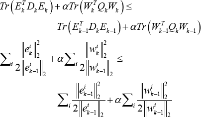
where E = X - XW, e ⁱ _k and w ⁱ _k are the i-th row of the matrices E, W. Moreover, D and Q are diagonal matrices whose i-th diagonal elements are D _ii = 1/2 ||e ⁱ ||₂ and Q _ii = 1/2||w ⁱ ||₂, respectively. Then the inequality in Eq. 21 holds.

$$\begin{array}{l}{\displaystyle \sum _i{\Vert e_k^i\Vert }_2}+\alpha {\displaystyle \sum _i{\Vert w_k^i\Vert }_2}-\left({\displaystyle \sum _i{\Vert e_k^i\Vert }_2}-{\displaystyle \sum _i\frac{{\Vert e_k^i\Vert }_2^2}{2{\Vert e_{k-1}^i\Vert }_2}}\right)-\alpha \left({\displaystyle \sum _i{\Vert w_k^i\Vert }_2}-{\displaystyle \sum _i\frac{{\Vert w_k^i\Vert }_2^2}{2{\Vert w_{k-1}^i\Vert }_2}}\right)\le \\ {\displaystyle \sum _i{\Vert e_{k-1}^i\Vert }_2}+\alpha {\displaystyle \sum _i{\Vert w_{k-1}^i\Vert }_2}-\left({\displaystyle \sum _i{\Vert e_{k-1}^i\Vert }_2}-{\displaystyle \sum _i\frac{{\Vert e_{k-1}^i\Vert }_2^2}{2{\Vert e_{k-1}^i\Vert }_2}}\right)-\alpha \left({\displaystyle \sum _i{\Vert w_{k-1}^i\Vert }_2}-{\displaystyle \sum _i\frac{{\Vert w_{k-1}^i\Vert }_2^2}{2{\Vert w_{k-1}^i\Vert }_2}}\right)\end{array}$$

Eq. 21

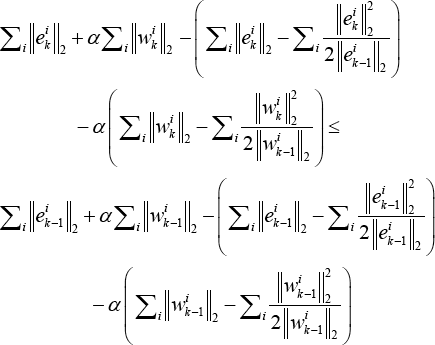
According to Lemma 1, it is easy to get the inequalities from Eq. 22.

$${\displaystyle \sum _i{\Vert e_k^i\Vert }_2}-{\displaystyle \sum _i\frac{{\Vert e_k^i\Vert }_2^2}{2{\Vert e_{k-1}^i\Vert }_2}}\le {\displaystyle \sum _i{\Vert e_{k-1}^i\Vert }_2}-{\displaystyle \sum _i\frac{{\Vert e_{k-1}^i\Vert }_2^2}{2{\Vert e_{k-1}^i\Vert }_2}}$$

Eq. 22

and Eq. 23.

$${\displaystyle \sum _i{\Vert w_k^i\Vert }_2}-{\displaystyle \sum _i\frac{{\Vert w_k^i\Vert }_2^2}{2{\Vert w_{k-1}^i\Vert }_2}}\le {\displaystyle \sum _i{\Vert w_{k-1}^i\Vert }_2}-{\displaystyle \sum _i\frac{{\Vert w_{k-1}^i\Vert }_2^2}{2{\Vert w_{k-1}^i\Vert }_2}}$$

Eq. 23

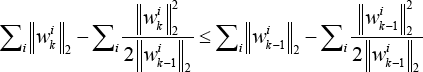
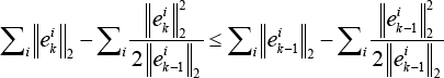
Adding Eqs. 22 and 23 into Eq. 21 gives Eq. 24.

$$\begin{array}{l}{\displaystyle \sum _i{\Vert e_k^i\Vert }_2}+\alpha {\displaystyle \sum _i{\Vert w_k^i\Vert }_2}\le {\displaystyle \sum _i{\Vert e_{k-1}^i\Vert }_2}+\alpha {\displaystyle \sum _i{\Vert w_{k-1}^i\Vert }_2}\\ \mathrm{Tr}\left(E_k^T{D}_k{E}_k\right)+\alpha \mathrm{Tr}\left(W_k^T{Q}_k{W}_k\right)\le \mathrm{Tr}\left(E_{k-1}^T{D}_k{E}_{k-1}\right)+\alpha \mathrm{Tr}\left(W_{k-1}^T{Q}_k{W}_{k-1}\right)\\ {\Vert E_k\Vert }_{2,1}+\alpha {\Vert W_k\Vert }_{2,1}\le {\Vert E_{k-1}\Vert }_{2,1}+\alpha {\Vert W_{k-1}\Vert }_{2,1}\\ {\Vert X-X{W}_k\Vert }_{2,1}+\alpha {\Vert W_k\Vert }_{2,1}\le {\Vert X-X{W}_{k-1}\Vert }_{2,1}+\alpha {\Vert W_{k-1}\Vert }_{2,1}\end{array}$$

Eq. 24

which indicates the objective function of Eq. 12 monotonically decreases under the updating rule of Algorithm 1.

JLE

By introducing the L_2,1-norm as the measurement into the objective function for linear embedding, it is expected that the linear representation in low-dimensional space could be more robust to the outliers compared with LPP, NPE, and SPP. After obtaining the sparse weight matrix W, we will construct the minimization objective function to optimize the projection matrix A. The designed objective function for jointly linear embedding is given in Eq. 25.

$$\underset{A}{\min }\Vert Y-WY{\Vert }_{2,1}$$

Eq. 25

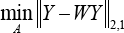
where Y = X ^T A, Y ∈ ℝ ^nxd , X ∈ ℝ ^rxn , A ∈ ℝ ^rxd and W ∈ ℝ ^nxn .

The L_2,1-norm imposed on the dominant term in Eq. 25 plays an important role for JLE. The objective function in Eq. 25 means that the samples in the low-dimensional space make use of the “sparse neighbors” for linear representation. Such “sparse neighbors” also exist on the low-dimensional space and indicated by the sparse weight matrix under the projection A. Unlike LPP, NPE, SPP, the proposed JLE uses the L_2,1-norm for measurement and the representation residuals in low-dimensional space are measured by L_2,1-norm to generate the projection matrix for reserving the crucial features in subspace learning.

Since Y = X ^T A, Eq. 25 can be transformed into Eq. 26.

$$\underset{A}{\min }{\Vert (I-W)X^{T}A\Vert }_{2,1}$$

Eq. 26

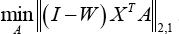
To remove an arbitrary scaling factor in the projection, we impose a constraint on the above optimization problem using Eq. 27.

$$\mathrm{Tr}\left(Y^{T}Y\right)=\text{ const}.$$

Eq. 27

where const. denotes a constant value. Combining Eqs. 26 and 27, we obtain an entire mathematical model for JLE as expressed in Eq. 28.

$$\underset{A}{\min }\mathrm{Tr}\left[A^{T}X{(I-W)}^{T}U(I-W)X^{T}A\right]\text{ s}.\text{t}.\mathrm{Tr}\left(A^{T}X{X}^{T}A\right)=\text{ const}.$$

Eq. 28

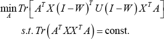
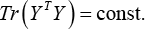
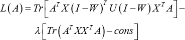
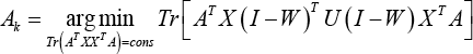
where U is a diagonal matrix whose diagonal element is U _ii = 1/2 ||p ⁱ ||₂ and p ⁱ is the i-th row of the matrix P = A ^T X (I - W) ^T . The constraint Tr (A ^T XX ^T A) = cons that we imposed on the proposed model can remove arbitrary scaling factors in the projection.

Using the Lagrange multiplier method, the constrained minimization problem can be converted to Eq. 29.

$$L(A)=\mathrm{Tr}\left[A^{T}X{(I-W)}^{T}U(I-W)X^{T}A\right]-\lambda \left[\mathrm{Tr}\left(A^{T}X{X}^{T}A\right)-cons\right]$$

Eq. 29

Taking the derivate of L(A) with respect to A and setting the formula to zero, we have Eq. 30.

$$\frac{\partial L}{\partial A}=2X{(I-W)}^{T}U(I-W)X^{T}A-2\lambda X{X}^{T}A=0$$

Eq. 30

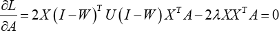
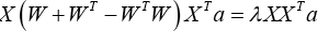
Therefore, the optimal variable A that minimizes the objective function Eq. 28 is given by the solution to the following generalized eigenvector problem with minimum eigenvalues in Eq. 31.

$$X{(I-W)}^{T}U(I-W)X^{T}A=\lambda X{X}^{T}A$$

Eq. 31

The overall description for obtaining the projection matrix is summarized in Algorithm 2.

Algorithm 2:

Solving the projection matrix

Input: X ∈ W ∈ ℝ nxn

1. Initialization: Set k = 0 and U0 = I.

2. Repeat:

3. Compute Ak+1 the matrix whose column vectors are the d eigenvectors of Eq. 31 associated with the d smallest nonzero eigenvalues.

4. Update the diagonal matrix [Uk+1, where the i-th diagonal element is U ii = (2||p i k+1||2)-1 and p i k+1 is the i-th row of the matrix Pk+1 = A T k+1X (I - W) T .

5. Let k ← k + 1.

6. Until convergence

Output: Projection vectors in matrix A ∈ ℝ rxd

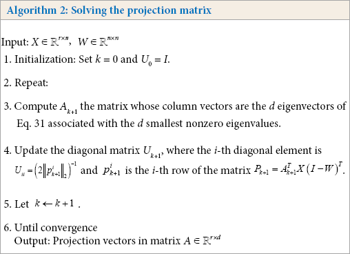
Then we give a theoretical analysis with regard to the convergence of Algorithm 2 as follows.

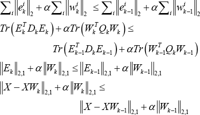
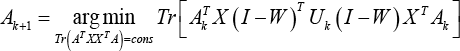
Theorem 2: For a given weight matrix W, the iterative approach in Algorithm 2 monotonically reduces the objective function value of optimization problem in Eq. 28 in each iteration.

Proof: According to the definition of A _k in Algorithm 2, we have Eq. 32.

$$A_k=\underset{\mathrm{Tr}\left(A^{T}X{X}^{T}A\right)=\text{ cons }}{\arg \min }\mathrm{Tr}\left[A^{T}X{(I-W)}^{T}U(I-W)X^{T}A\right]$$

Eq. 32

Since P = A ^T X(I - W) ^T , Eq. 32 can be further transformed to Eq. 33

$$A_{k+1}=\underset{\mathrm{Tr}\left(A^{T}X{X}^{T}A\right)=\text{ cons }}{\arg \min }\mathrm{Tr}\left[A_k^{T}X{(I-W)}^T{U}_k(I-W)X^T{A}_k\right]$$

Eq. 33

which means that Eqs. 34 and 35 are valid.

$$\mathrm{Tr}\left(P_{k+1}{U}_k{P}_{k+1}^T\right)\le \mathrm{Tr}\left(P_k{U}_k{P}_k^T\right)$$

Eq. 34

That is to say,

$${\displaystyle \sum _i\frac{{\Vert p_{k+1}^i\Vert }_2^2}{2{\Vert p_k^i\Vert }_2}}\le {\displaystyle \sum _i\frac{{\Vert p_k^i\Vert }_2^2}{2{\Vert p_k^i\Vert }_2}}$$

Eq. 35

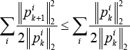
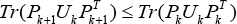
where vectors p ⁱ _k and p ⁱ _k+1 indicate the i-th rows of the matrices P _k and P_k+1, respectively.

On the other hand, according to Lemma 1, for each i, we have Eq. 36.

$${\displaystyle \sum _i{\Vert p_k^i\Vert }_2}-{\displaystyle \sum _i\frac{{\Vert p_k^i\Vert }_2^2}{2{\Vert p_{k-1}^i\Vert }_2}}\le {\displaystyle \sum _i{\Vert p_{k-1}^i\Vert }_2}-{\displaystyle \sum _i\frac{{\Vert p_{k-1}^i\Vert }_2^2}{2{\Vert p_{k-1}^i\Vert }_2}}$$

Eq. 36

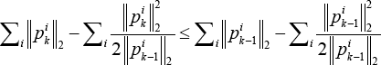
Combining Eqs. 35 and 36, we further have Eq. 37,

$${\displaystyle \sum _i{\Vert p_k^i\Vert }_2}\le {\displaystyle \sum _i{\Vert p_{k-1}^i\Vert }_2}$$

Eq. 37

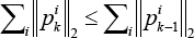
that is to say (Eq. 38),

$${\Vert Q_{k+1}\Vert }_{2,1}\le {\Vert Q_k\Vert }_{2,1}$$

Eq. 38

and namely Eq. 39.

$${\Vert A_{k+1}^{T}X{(I-W)}^T\Vert }_{2,1}\le {\Vert A_k^{T}X{(I-W)}^T\Vert }_{2,1}.$$

Eq. 39

Thus, Algorithm 2 will monotonically reduce the objective of the problem (Eq. 26) in each iteration.

Comparisons between NPE, SPP, and the Proposed Method

JLE and the representative dimensionality reduction methods NPE and SPP have something in common. They all discover the potential structure among the data manifold during the process of subspace learning. However, JLE is different from NPE and SPP in the following aspects.

1. 1)

NPE finds the L₂-norm-based local reconstruction relation and SPP finds the L₁-norm-based sparse reconstruction relation. Although JLE also finds the sparse reconstruction relation among the data points, such a relation is derived by using the jointly sparse learning based on the L_2,1-norm.

2)

The way of JLE weight matrix learning is different from NPE and SPP. Both NPE and SPP have to obtain the weight vector one-by-one via solving the regression problem, where the former uses the L₂-norm to measure the representation residual, and the later uses the L₁-norm to solve the sparse weight vector. In JLE, the learning of the sparse weight vectors is performed in batch mode, namely, the sparse weight matrix can be obtained directly by solving the L_2,1-norm-based jointly sparse learning model.

3)

Furthermore, both NPE and SPP use the L₂-norm to measure the representation residual of the low-dimensional data during the phase of projection matrix learning. However, JLE adopts the L_2,1-norm to perform jointly linear embedding for projection learning. The linear representation in low-dimensional space is more robust to the outliers compared with that of NPE and SPP.

Experimental Results

To validate the real classification performance of JLE, we conducted comparison experiments on the ORL, ⁵² Yale, ⁵³ AR ⁵⁴ , and PIE ⁵⁵ face databases, and XueLang fabric defect database. ⁵⁶ The representative dimensionality reduction methods, including LPP, ¹⁸ NPE, ¹⁹ and SPP, ³⁰ were used for comparison. The Neighborhood Preserved LLE (NLLE), ⁵⁷ Linear Projection Direction-based NPE(LPNPE), ⁵⁸ and Subspace-based Ensemble Sparse Representation (RS_ESR) ⁵⁹ were further used for validating the effectiveness of the proposed method on noisy data. The experimental results shown in the following subsections support our novel viewpoint that the proposed method is competitive with other state-of-the-art methods for visual classification. For the face databases, the corresponding descriptions are summarized in Table I. For the fabric defect database, we classify the defect types to evaluate the performance of the proposed method. In the experiments, the recognition rate was exploited to measure the performance of the algorithm. The training process is randomly repeated 10 times and then the average recognition rates were computed and reported.

Table I.

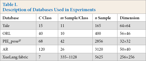
Description of Databases Used in Experiments

Database	C Class	m Sample/Class	n Sample	Dimension
Yale	15	11	165	64x64
ORL	40	10	400	56x46
PIE_pose 27	68	42	2856	32x32
AR	120	26	3120	50x40
XueLang fabric	7	335∼1128	5625	256x256

Four Face Databases

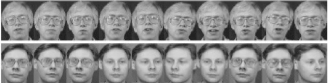
The ORL face database ⁵² totally has 400 frontal-face images of 40 individuals and provides a variety of facial expressions and facial details (e.g., glasses or no glasses). In the experiments, all the images were normalized to a resolution of 56x46. Part of the face samples in the ORL face database are shown in Fig. 1.

Fig. 1

Sample images of two people from the ORL database.

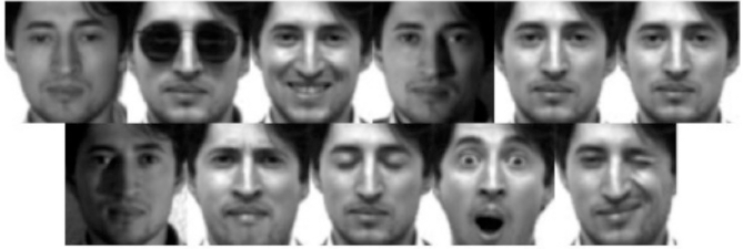
The Yale database has a total of 165 gray scale images of 15 individuals. ⁵³ Each subject contains 11 images with different facial situations including wearing glasses, left lighting, surprised, sad and so on. All the images were normalized to a resolution of 64x64 for the experiments. Sample images of the Yale face database are shown in Fig. 2.

Fig. 2

Sample images of one person from the Yale database.

The number of face images in the AR database is over 4000. ⁵⁴ All images are provided by 126 people, including 70 men and 56 women, with abundant facial expressions, occlusions, and lighting changes. In this study, we used the face images of 120 people (65 men and 55 women) for the experiments. The images were taken in two sessions and each section contained 13 images. For each image, it was normalized to a resolution of 50x40 for further processing. Some of the ORL face images are shown in Fig. 3.

Fig. 3

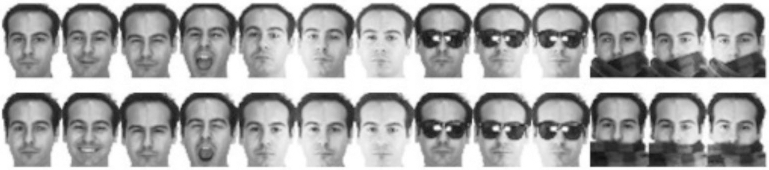
Sample images of one person from the AR face database.

For the CMU PIE database, ⁵⁵ the face images of 68 people are provided, where each person has 13 pose variations and 43 different lighting conditions. In this study, the PIE images of 68 people were used, but only a portion of face images (42 facial images) with lighting changes were adopted for the experiments. Moreover, we extracted the face targets from the PIE face images and then converted them into a size of 32x32 for this work. The PIE face images with strong lighting changes are shown in Fig. 4.

Fig. 4

Sample images of one person from PIE face database.

XueLang Fabric Defect Database

The XueLang fabric defect database ⁵⁶ contains over nine defect types. In this experiment, we divided the defects into seven defect types, namely float, hole, missing_end, missing_pick, draw_back_end, weft_crackiness, and normal types. All defects were collected in the factory. The visual images of the defects are shown in Fig. 5. The resolution of these defect images are 256x256.

Fig. 5

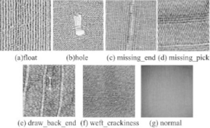
Seven defect types of XueLang fabric defect database.

Parameter Tuning

We used the popular dimensionality reduction methods for comparisons: 1) LPP, ¹⁸ 2) NPE, ¹⁹ 3) SPP, ³⁰ the proposed 4) JLE, 5) NLLE, ⁵⁷ 6) LPNPE, ⁵⁸ and 7) RS_ESR. ⁵⁹

For the four face databases, we randomly selected 20% to 80% of the images per class for training, and the remaining for testing. For the defect database, we selected 100 defect images for training and 30 defect images for testing in seven classes. With the given training set, the projection matrix A was learned by the comparison methods, respectively, and the test samples were subsequently transformed by the learned projection matrix. In the classification stage, we used the 1NN classifier to evaluate the recognition rates on the test data.

For LPP algorithm, the neighborhood size k was searched from {5, 10, 15, 20} and the kernel width t was set to the mean norm of the training data. To preserve the main energy of the samples, PCA was used to extract the principal components. For the NPE algorithm, the neighborhood size k was searched from {5, 10, 15, 20}. The SPP algorithm was parameter-free. For NLLE, LPNPE, and RS_ESR, we used the default parameters specified by the original paper. For the proposed JLE algorithm, the experiments were also conducted after the extraction of principal components of the original data by PCA. Furthermore, the regularization parameter α in JLE was searched from {10^-10, 10^-9, … 10 ¹⁰ } and the best results were reported.

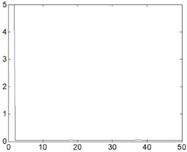
For ORL, Yale, PIE, AR, and XueLang databases, the parameters α of the best results were set to 10^–1, 10^-2, 10^-7, 10^-2, and 10^-3 respectively. Fig. 6 shows the variation of the recognition rate versus the values of α (Alpha), which demonstrates that the proposed method is insensitive to the variation of the parameter.

Fig. 6

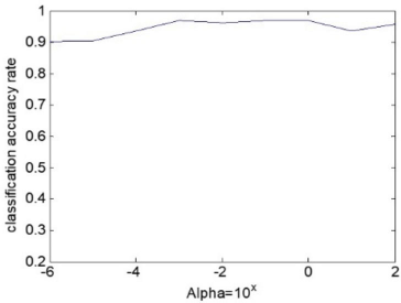
The recognition rates vs. the value of Alpha.

Convergence Analysis

As proven in the previous section, the updating rules in Algorithms 1 and 2 guarantee an optimum solution for our objective functions defined in Eqs. 14 and 29. We drew the convergence curves of weight matrix learning and projection matrix learning of JLE in Figs. 7 and 8, respectively, which show that the objective function value decreases with the increase of the iteration number on the ORL database. We also observed that Algorithms 1 and 2 converge rapidly after 10 iterations. Therefore, we set the maximum iteration number of Algorithms 1 and 2 to 50 in the following experiments.

Fig. 7

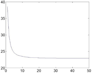
The objective function of Algorithm 1 for constructing the weight matrix W on ORL database. Objective function value decreases along with the increase of the iteration number.

Fig. 8

The objective function value of Algorithm 2 for obtaining the projection matrix A on ORL database. Objective function value decreases very fast with the increase of the iteration number.

Visualization of Sparse Weight Matrix

We also evaluated the sparsity property of the weight matrix for the proposed JLE method. Fig. 9 shows that weight matrix W is sparse and, most important of all, the majority of the nonzero coefficients are well aligned along the diagonal direction of the weight matrix, which shows that the proposed JLE is able to explore the naturally discriminative information for dimensionality reduction, even if no class labels are included.

Fig. 9

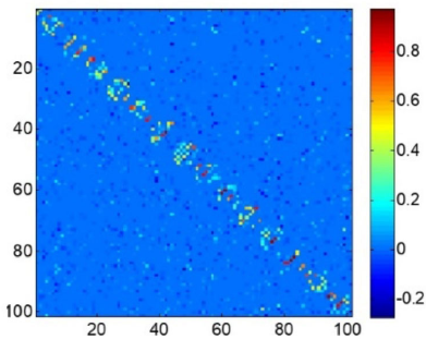
The part of weight matrix W obtained by Algorithm 1 on ORL database.

Experimental Results on Four Databases

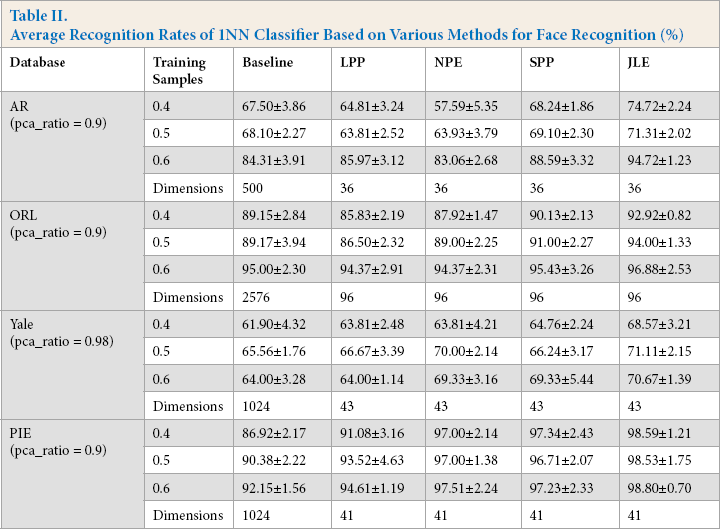
For the four face databases, we randomly select 20% to 80% of the images per class for training, and the remaining for testing. The maximal average recognition rate of each method and the corresponding dimension are shown in Fig. 10 and Table II. Fig. 10 shows the accuracies of the various methods with various proportions of training samples on four databases. Table II shows some detailed recognition rates of the experiments, among which the numerical values 0.4, 0.5, and 0.6 in the table represent 40%, 50%, and 60% of the images per class were randomly selected for training.

Table II.

Average Recognition Rates of 1NN Classifier Based on Various Methods for Face Recognition (%)

Database	Training Samples	Baseline	LPP	NPE	SPP	JLE
AR (pca_ratio = 0.9)	0.4	67.50±3.86	64.81±3.24	57.59±5.35	68.24±1.86	74.72±2.24
	0.5	68.10±2.27	63.81±2.52	63.93±3.79	69.10±2.30	71.31±2.02
	0.6	84.31±3.91	85.97±3.12	83.06±2.68	88.59±3.32	94.72±1.23
	Dimensions	500	36	36	36	36
ORL (pca_ratio = 0.9)	0.4	89.15±2.84	85.83±2.19	87.92±1.47	90.13±2.13	92.92±0.82
	0.5	89.17±3.94	86.50±2.32	89.00±2.25	91.00±2.27	94.00±1.33
	0.6	95.00±2.30	94.37±2.91	94.37±2.31	95.43±3.26	96.88±2.53
	Dimensions	2576	96	96	96	96
Yale (pca_ratio = 0.98)	0.4	61.90±4.32	63.81±2.48	63.81±4.21	64.76±2.24	68.57±3.21
	0.5	65.56±1.76	66.67±3.39	70.00±2.14	66.24±3.17	71.11±2.15
	0.6	64.00±3.28	64.00±1.14	69.33±3.16	69.33±5.44	70.67±1.39
	Dimensions	1024	43	43	43	43
PIE (pca_ratio = 0.9)	0.4	86.92±2.17	91.08±3.16	97.00±2.14	97.34±2.43	98.59±1.21
	0.5	90.38±2.22	93.52±4.63	97.00±1.38	96.71±2.07	98.53±1.75
	0.6	92.15±1.56	94.61±1.19	97.51±2.24	97.23±2.33	98.80±0.70
	Dimensions	1024	41	41	41	41

Fig. 10

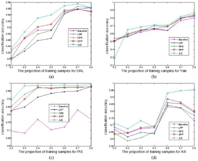
The classification accuracies of four database with different portions of training samples. (a) ORL, (b) Yale, (c) PIE, and (d) AR.

The performance of JLE was greater than the other methods in four databases using various numbers of training samples, as shown in Table II. Specially, the competitive recognition rate was obtained in the AR database when 60% training samples were used. The recognition rate of JLE was around 6% higher than that of the SPP, ranked in second place. Fig. 10 shows that the overall performance of JLE increased with the increased proportion of training samples. Even though databases such as AR and PIE contain an abundance of facial expressions and illumination variations, the proposed method was still superior to other state-of-the-art methods. The reason lies in the L_2,1-norm-based objective function and weight matrix that select the most important discriminative data or features to enhance the recognition rate, even under situations with complexities.

Experimental Results on XueLang Defect Database

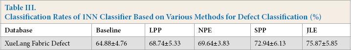
For the defect database, we selected 100 defect images for training and 30 defect images for testing in seven classes. In the experiment, ResNet ⁶⁰ was used to extract the deep features (the dimensionality is 2048x1) from defect images, and thus PCA was used to reduce the dimensionality of the features so that the computation can be fluently conducted on our computing platform. The experimental results of different methods on the XueLang defect database are shown in Table III. It shows that the proposed method was competitive with the popular dimensionality reduction methods on the classification task.

Table III.

Classification Rates of 1NN Classifier Based on Various Methods for Defect Classification (%)

Database	Baseline	LPP	NPE	SPP	JLE
XueLang Fabric Defect	64.88±4.76	68.74±5.33	69.64±3.83	72.94±6.13	75.87±5.85

Experimental Results Including Outliers

To evaluate the performance of the JLE algorithm when face images are occluded with outliers, we added a 10x10 noise block on the original face images in four databases. The position of the noise block on every face image was set randomly. In Fig. 11, we show some occlusion images from the ORL database. To evaluate the performance of JLE and other dimensionality reduction methods including LPP, NPE, and SPP, we conducted the experiments on the newly-created occlusion databases.

Fig. 11

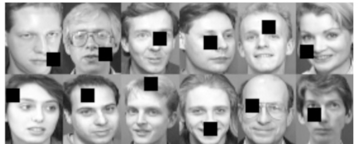
Sample images of the occlusion ORL database.

The experimental setting and parameter tuning were the same as the above experiments performed on the original face databases. Specially, the parameter α on the ORL, Yale, PIE, and AR databases were set to 10, 1, 100, and 0.01, respectively.

Fig. 12 shows the accuracies of various methods with various proportions on training samples for the four databases, and a detail report is shown in Table IV. From Table IV, the proposed method was not the best (only 0.15% lower than the best one) when 40% of the training samples were used in the AR database. However, with the increased number of training samples, JLE showed its superiority over the other methods as shown by the results using the AR database in Table IV. It should be noted that the fluctuations of all the recognition accuracies using outliers were more severe than that of the results in Table II. The random positions of noise blocks had a great influence on the performance of all comparison methods, which resulted in a decreased problem of recognition accuracies. For example, the average recognition rate 61.25% with 60% training samples was less than the average recognition rate of 62.50% when 50% training samples were used from the ORL database, as shown in Table IV. However, such discrepancies were not so great and still in a reasonable range under the influence of noise blocks.

Table IV.

Average Recognition Rates of 1NN Classifier Based on Various Methods for Face Recognition (%)

Database	Training Samples	Baseline	LPP	NPE	SPP	JLE
AR (pca_ratio = 0.9)	0.4	39.81±5.55	41.85±4.68	46.20±3.08	42.78±3.74	46.05±2.82
	0.5	35.71±4.18	38.10±6.60	39.64±4.38	38.69±2.06	40.55±2.32
	0.6	47.50±7.00	56.67±5.16	54.58±2.96	52.86±4.08	57.72±2.55
	Dimensions	500	36	36	36	36
ORL (pca_ratio = 0.9)	0.4	53.75±4.50	50.42±3.33	50.00±3.68	59.58±3.76	62.08±1.83
	0.5	52.00±3.38	50.50±5.85	55.50±2.05	61.00±2.66	62.50±2.08
	0.6	53.75±3.83	54.38±3.71	58.75±3.12	60.00±2.87	61.25±2.68
	Dimensions	2576	96	96	96	96
Yale (pca_ratio = 0.98)	0.4	33.33±6.17	38.10±6.93	38.10±2.56	37.14±3.32	40.95±2.54
	0.5	33.33±5.67	34.44±3.66	40.00±5.04	33.33±2.24	46.67±3.06
	0.6	36.00±3.53	40.00±4.24	36.25±2.84	40.00±4.94	48.00±2.62
	Dimensions	1024	43	43	43	43
PIE (pca_ratio = 0.9)	0.4	35.29±5.75	36.96±5.52	36.79±3.96	41.23±5.26	60.21±2.60
	0.5	35.57±4.57	36.23±4.05	37.37±4.06	40.83±3.42	63.52±1.38
	0.6	38.32±4.75	39.04±3.62	40.32±3.30	47.84±2.28	63.15±3.40
	Dimensions	1024	41	41	41	41

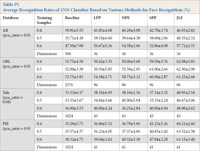
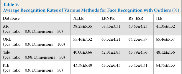
Even though the performance of all methods were affected by these outliers, the performance of JLE was competitive with other state-of-the-art methods, with an increased proportion of training samples, as shown in Fig. 12. It should be noted that JLE had very good performance using the Yale and PIE databases under the influence of noise blocks. The average recognition rate of JLE was at least 8% and 16% higher than LPP and SPP when 60% of the noisy training samples were used with Yale and PIE databases, respectively. We further validated the effective-ness of JLE by comparing it with NLLE, LPNPE, and RS_ESR on the image data with outliers in four face databases, among which 50% of the samples were used for training. The experimental results in Table V shows that JLE was more competitive than the state-of-the-art methods. Based on Fig. 12 and Tables IV and V, our algorithm achieved the best result, and the classification accuracies were obviously higher than other methods.

Fig. 12

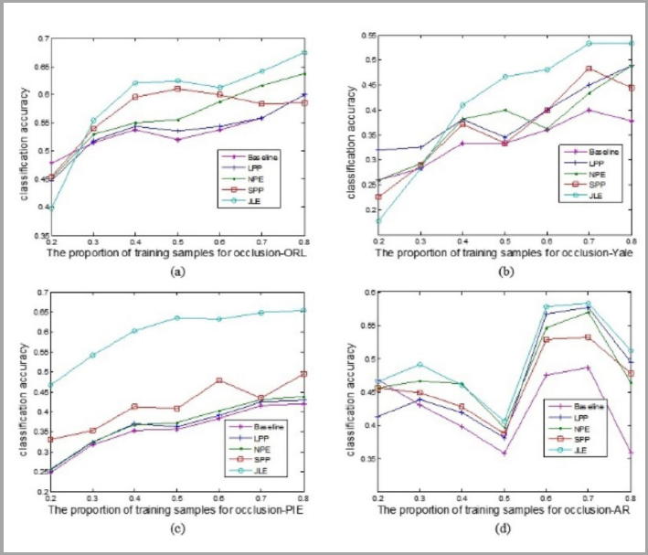
Accuracies of various methods with various proportions on training samples for the four databases.

Table V.

Average Recognition Rates of Various Methods for Face Recognition with Outliers (%)

Database	NLLE	LPNPE	RS_ESR	JLE
AR (pca_ratio = 0.9, Dimensions = 50)	38.25±5.35	38.45±3.31	40.65±4.23	41.35±4.32
ORL (pca_ratio = 0.9, Dimensions = 100)	55.46±7.32	60.32±4.21	64.23±6.57	65.46±5.37
Yale (pca_ratio = 0.98, Dimensions = 50)	40.00±3.66	42.01±2.83	43.79±4.56	48.12±2.56
PIE (pca_ratio = 0.9, Dimensions = 50)	43.39±6.48	48.32±6.43	55.43±8.31	64.75±4.53

Conclusion

In this study, we proposed a new algorithm called Joint Linear Embedding (JLE) for dimensionality reduction based on the L_2,1-norm. In the proposed algorithm, the weight matrix obtained by optimizing an L_2,1-norm-based objective function is sparse and the L_2,1-norm-based loss function is robust to outliers. The L_2,1-norm-based regularization can select the related samples with latent discriminant information due to the strong ability of the L_2,1-norm for jointly sparse learning. During the projection learning phase, JLE was performed based on the L_2,1-norm, which showed robust representation ability against the outliers compared with LPP, NPE, SPP, NLLE, LPNPE, and RS_ESR. And such robustness was further validated by the results in the experimental section.

In this work, the L_2,1-norm was integrated into the dimensionality reduction framework for jointly sparse learning and jointly linear embedding. We also provided the theoretical proof of the convergence of JLE. In the future, to obtain a more robust dimensionality reduction method against the outliers, a sparse projection matrix with the ability of feature extraction and selection will be designed for linear embedding.