Detection of Phenotypic Alterations Using High-Content Analysis of Whole-Slide Images

Abstract

Tumors exhibit spatial heterogeneity, as manifested in immunohistochemistry (IHC) staining patterns. Current IHC quantification methods lose information by reducing this heterogeneity in each whole-slide image (WSI) or in selective fields of view to a single staining index. The aim of this study was to investigate the sensitivity of an IHC quantification method that uses this heterogeneity to reliably compare IHC staining patterns. We virtually partitioned WSIs by a grid of square tiles, and computed the staining index distributions to quantify heterogeneities. We used samples from these distributions as inputs to non-parametric statistical comparisons. We applied our grid method to fixed tumor samples from 26 tumors obtained from a double-blind preclinical study of a patient-derived orthotopic xenograft model of pediatric neuroblastoma in CD1 nude mice. We compared the results of our grid method to the results based on whole-slide indices, the current practice. We show that our grid method reliably detects phenotypic alterations that other tests based on whole-slide indices fail to detect. Based on robustness and increased sensitivity of statistical inference, we conclude that our method of whole-slide grid quantification is superior to existing whole-slide quantification techniques.

Introduction

Immunohistochemical (IHC) markers are integral to computational pathology, an emergent discipline (Louis et al. 2014). IHC markers are key tools in clinical research and practice (decision making (Walsh et al. 2008; Sheri and Dowsett 2012; Prescott 2013), diagnostic and treatment evaluation and prognosis (Mulrane et al. 2008; Polcher et al. 2010; Madabhushi et al. 2011)), translational research (drug discovery and development (Fuchs et al. 2008; O’Connor et al. 2008; Sullivan and Chung 2008; Dolled-Filhart and Gustavson 2012; Hewitt 2012; Prescott 2013; Shinde et al. 2014; Smith and Womack 2014)) and basic science, especially in cancer research (Faratian et al. 2011; Dolled-Filhart and Gustavson 2012). With the advent of individualized cancer therapy (e.g., targeted therapy), characterization of individual tumors and their alterations in response to therapies is essential. Specifically, IHC staining indices (often defined as the percentage of positively stained cells among total counted cells in the field(s) of view) are widely used as prognostic factors in clinical practice (Fitzgibbons et al. 2000; Taylor and Levenson 2006; Matos et al. 2010; Inwald et al. 2013).

Recent studies have shown potential new applications by comparing IHC tissue staining indices before and after therapy. A retrospective study of ovarian cancer patients has shown changes in tissue staining indices induced by treatment to be stronger predictors of clinical outcomes than baseline indices alone (Polcher et al. 2010; Sheri and Dowsett 2012). In a randomized phase II clinical trial for breast cancer, changes in the Ki67 index evaluated from biopsied specimens after 2 weeks of preoperative chemotherapy has been used to guide the selection of a subsequent chemotherapy regimen (Yamaguchi and Mukai 2012). These new applications may benefit from accurate quantification and comparison of IHC patterns before and after treatment, as opposed to the comparison of two indices that average over underlying intra-tumor phenotypic heterogeneity (Marusyk et al. 2012).

One of the greatest challenges in the quantification of staining indices is the selection of fields in the presence of intra-tumor heterogeneity. A number of methods have been used for selecting fields of view for quantification (Uzzan et al. 2004; Pathmanathan and Balleine 2013). These methods often involve looking for highly active regions (called ‘hot-spots’) and selecting multiple fields within those regions, leading to subjectivity of measurements. This makes inferences biased and therefore unreliable. Whole-slide imaging (digitizing the entire glass slide) and whole-slide quantification (analyzing all relevant tissue on the slide) are emerging as potential solutions to minimize this subjectivity by including entire histological sections (as reviewed in (Kothari et al. 2013; Webster and Dunstan 2014)). There are a number of commercial and open-source solutions that provide a whole-slide staining index (the percentage of positively stained cells among total counted cells in a tissue of interest). Region(s) of interest (ROI) are selected either manually or automatically over the entire slide using pattern recognition algorithms. The most common analysis packages with varying levels of flexibility are: Aperio’s Image Analysis Toolbox (Aperio Technologies), inForm (PerkinElmer, Waltham, MA), Tissue Studio and Definiens Developer (Definiens, Carlsbad, CA), Visiopharm (Hoersholm, Denmark), Matlab (MathWorks, Natick, MA) and ImageJ (NIH).

The ROIs used for whole-slide quantification often include regions with heterogeneous IHC patterns and histological properties. These heterogeneities may contain useful information (Potts et al. 2012). This information is lost when we calculate averaged indices over such ROIs. Averaged indices are appropriate descriptors only if the underlying patterns are homogeneous (e.g., spatially uniformly random pattern or spatially uniform pattern (Diggle 2013)). Using smaller ROIs provides local quantification and therefore better represents the phenotypic heterogeneities. For instance, Nawaz et al. (2015) stratified patients based on spatial heterogeneity of immune cells in estrogen receptor-negative breast cancer. However, in the absence of automated tools, manual efforts quickly become tedious owing to the large numbers of such ROIs required for reliable statistical comparisons.

Recently, spatial statistics has been used to analyze patterns in biological images (IHC and immunofluorescent images) (Mattfeldt 2011; Mattfeldt et al. 2013; Burguet and Andrey 2014). This class of analysis involves making certain assumptions about the underlying biological patterns (homogeneity vs aggregation) and fitting a limited number of known spatial patterns to estimate model parameters and their confidence intervals. The most common spatial model is uniform random distribution (Poisson spatial process) with one parameter that corresponds to the staining index. Mattfeldt et al. (2013) have analyzed spatial processes using bootstrapping techniques by estimating the IHC staining index of spatial patterns and their confidence intervals. In this method, spatial patterns with different intensities and non-overlapping confidence intervals (NCIs) are statistically different. But selecting appropriate non-homogeneous spatial models to fit observed patterns for statistical comparison is not trivial. Mechanisms of pattern formation must be hypothesized to formulate appropriate spatial models. Another complicating factor is that IHC patterns contain different classes of spatial heterogeneity within the same slide (tissue section) and across a cohort (analysis of replicated patterns), which makes it even more difficult to fit a single spatial model. Spatial analysis often requires geometrically simple, contiguous regions and applies complex schemes to correct for edge effects. These requirements are usually not met in IHC patterns (see viable tumor regions separated by necrotic regions; Fig. 2). Making assumptions about pattern formation mechanisms, choosing a multi-parametric model and fitting lack robustness.

Manual and automated stereology (Gardi et al. 2008) provide a number of unbiased techniques to estimate histological and IHC properties in 2D and 3D. These well-established techniques are designed to work with heterogeneous patterns and provide invaluable information about the structure and function of cells, tissues and organs. A class of stereological techniques provides tools to estimate the count of objects in a 3D volume (e.g., number of brain cells within a brain region). These estimates are based on a sum of objects counted in the counting frames that are spatially distributed according to a sampling grid over the tissue. The spatial heterogeneity captured by these individual counts per counting frames is lost when they are summed to a single number for each tissue sample.

In summary, the shortcomings of existing methods are their lack of reliability, their lack of robustness, and a loss of information. This motivated our development of a reliable, model-free technique that quantitatively compares phenotypic properties of tissue, which accounts for underlying heterogeneities.

We present a robust method to quantify and compare phenotypic tissue properties as measured by IHC staining indices. We virtually partitioned the whole-slide images (WSIs) into a set of small square tiles and computed the distributions of staining indices to represent tissue heterogeneities. We used samples from these distributions as inputs to non-parametric statistical comparisons. We applied our quantification methods to detect statistically significant phenotypic alterations resulting from Standard of Care (SOC) chemotherapy in a double-blinded preclinical study on a patient-derived orthotopic xenograft model of pediatric neuroblastoma (Stewart et al. 2015). We show that statistical tests based on our grid quantification method are able to detect alterations that other tests based on whole-slide indices fail to detect.

Materials & Methods

Animal Study

We used tissue samples from 26 CD1 nude mice (Charles River) from a randomized double-blind study (Stewart et al. 2015) from two treatment arms: placebo and standard of care (SOC). All the animal procedures were performed according to our IACUC-approved protocol. We used ultrasound-guided injection to implant 200,000 patient-derived neuroblastoma cells (suspended in MatriGel) orthotopically in the para-adrenal space (Teitz et al. 2011). Mice were enrolled in the study when tumors were first detected by regular ultrasound imaging every three weeks. Mice exited from the study if the tumor burden reached 20% of the body weight or if they became ill (e.g., 20% weight loss, lethargy, and persistent dehydration) or died. Tumors were imaged using VisualSonics VEVO 2100 ultrasound every three weeks from the enrollment date. SOC regimen included two 3-week courses (the first at 6 weeks after enrollment). Mice only received drugs during the first week of each course (no drugs for weeks 2 and 3 of each course). Mice in the SOC arm received cyclophosphamide (125 mg/kg, days 1 and 2), Adriamycin (3.5 mg/kg, day 1) and etoposide (6 mg/kg, days1–4) for courses 1 and cisplatin (2 mg/kg, days 1–5) and etoposide (5 mg/kg, days 2–4) for courses 2.

Immunohistochemistry

We harvested the tumor mass and fixed in 10% formalin. We processed and embedded the tissue slices in paraffin and prepared three sets of 4-µm-thick serial sections from each block. The serial section sets were 200 µm apart. Within each serial section set, we used 4 sections (one section per stain) to identify: 1) cellular apoptosis, by staining for activated caspase 3 (CASP3); 2) mitosis, by staining for phosphor-histone H3 (H3); 3) proliferation, by staining for Ki67; 4) blood vessels, by staining for CD34. We counterstained the slides with hematoxylin and eosin (H&E) to show cellular and tissue structures. The list of antibodies, staining instrumentation and protocols we used are provided in Supplemental Table S2.

Overview of Image Processing and IHC Quantification

Our image processing method includes three main steps: 1) slide scanning and preprocessing, 2) tissue classification, 3) IHC marker detection. We briefly discuss the image processing steps in the following sections and provide a more detailed description in the supplemental material. To quantify IHC for a tissue section, we virtually partition the classified WSI using grids (Fig. 1) into many tiles and calculated an IHC staining index for each grid tile. We formed a distribution from grid tile IHC indices and sampled from the distribution to run statistical tests.

Figure 1.

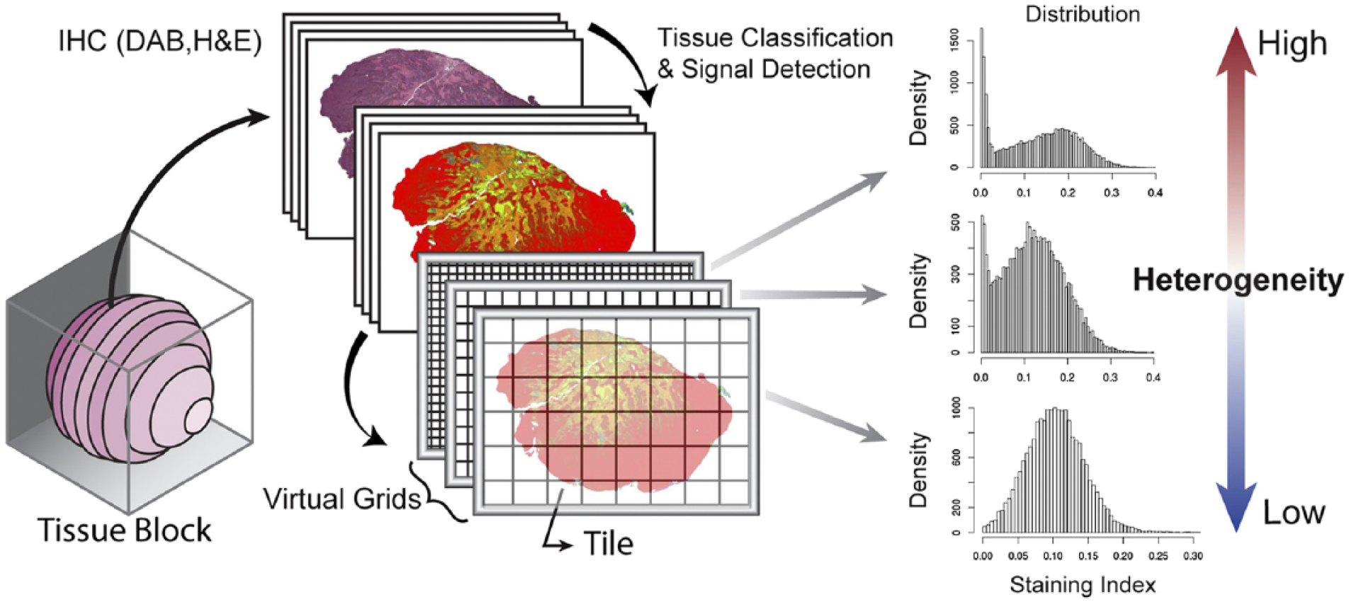
Multi-scale sampling and heterogeneity. Tumor tissue sampled to make a multiple tissue block. Serial sections were made from each block, which were stained with DAB and counterstained with H&E. Whole-slide sections were classified, and IHC index distributions were quantified using three grid tile sizes. Heterogeneity in IHC index decreases as tile size increases.

Slide Scanning and Preprocessing

We digitally scanned all the slides at 20× (objective lens) magnification using an Aperio ScanScope scanner (at this magnification, 1 pixel is 0.5 µm). We downsized the scanned images to 10× magnification for all IHC quantifications. We applied a color deconvolution technique (Ruifrok and Johnston 2001) to each image using our custom color vectors into three color channels: eosin (pink-orange), hematoxylin (blue-purple) and 3,3’-diaminobenzidine (DAB, brown) (we computed the custom color vector from three slides, each stained with one of DAB, H or E). We used the three color channels for tissue classification and IHC quantification. We used Fiji (Schindelin et al. 2012) for the entire image processing in the study.

Tissue Classification

IHC indices in this study were calculated over viable tumor regions. We developed a machine learning-based tissue classifier using Fiji (Schindelin et al. 2012) to identify viable tumor regions (Fig. 2). We used the staining and texture features in the slides stained with Ki67 (counterstained with H&E) within each set to classify the tissue into one of three types (Fig. 2): viable tumor tissue, necrotic tissue, and background (stroma, fat, tissue folds, liver, kidney, glass, spleen and muscle). We used 5× magnification images (1 pixel, ~2 µm) for creating the training set, developing tissue classifiers, and in the final application of the validated classifier on target images (for details see Supplemental Material). The final version of our classifier achieved 95% accuracy per region in a 10-fold cross-validation test (Refaeilzadeh et al. 2009). Based on results of our tissue classifier, the mean viable tumor tissue areas per WSI for the placebo and SOC arms were 29 ± 13 mm² and 32 ± 15 mm², respectively. The mean necrotic tissue areas per WSI for the placebo and SOC arms were 20 ± 16 mm² and 8 ± 7 mm², respectively.

Figure 2.

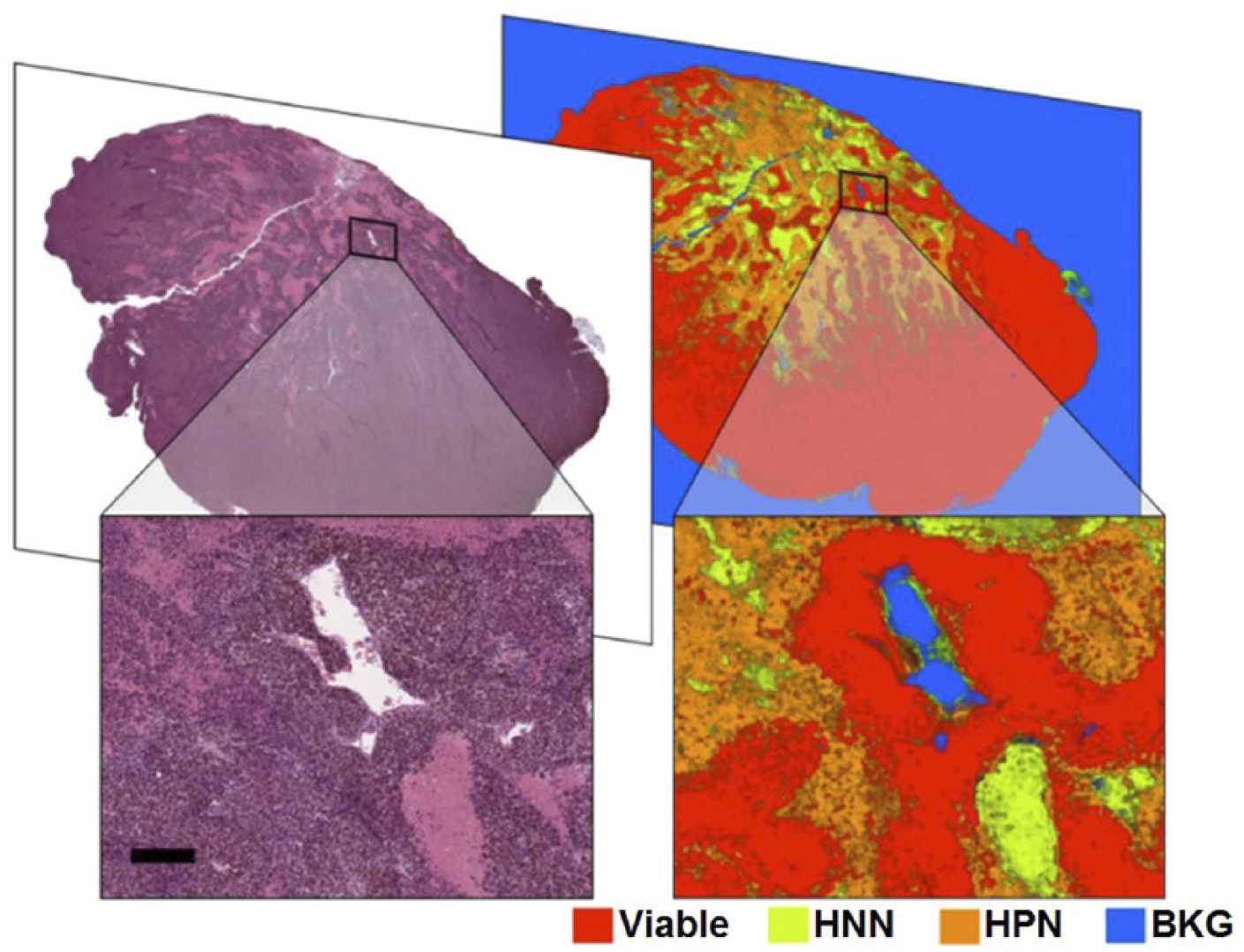
Whole-slide tissue segmentation output. Tissue section stained for Ki67 with H&E as counterstains. The nuclei of cells that have been necrotic for the longest time only lightly stain with hematoxylin (hematoxylin-negative necrotic (HNN) regions). Cells with small, intensely dark nuclei (DNA condensation) are generally dead or advanced in the process of dying (hematoxylin-positive necrotic (HPN) regions). Red, live tumor; yellow, H-negative necrotic (long-standing necrotic); orange: H-positive necrotic (HPN, forming necrotic); blue: background (BKG). Scale, 200 µm.

IHC Marker Detection

Manual or automated intensity threshold by a constant is often used to detect DAB-positive pixels in an image. This method is prone to error in the presence of nonspecific DAB staining. We used a classifier to detect DAB-positive pixels and minimize background noise due to nonspecific DAB staining. We used a training set at 10× magnification by sampling from a wide range of DAB intensities in the absence and presence of nonspecific staining, which usually occurs at tissue folds and edges. The final version of our DAB signal detection classifier achieved 99% accuracy in a 10-fold cross-validation test. We used the segmented image as a mask and applied it to the unmodified DAB-channel (straight out of deconvolution) to eliminate noise.

Multi-scale IHC Quantification and Statistical Tests

We investigated the effect of ROI sizes on the resulting staining index distributions and statistical tests by virtually partitioning the images using multiple non-overlapping square grids (Figure 1) at grid tile sizes ranging from 50 µm to 1000 µm. For each grid tile, we calculated staining indices as the ratios of total DAB-positive pixels in viable tumor tissue regions to the count of all pixels of viable tumor regions. To obtain viable tumor regions, we did spline-based elastic registration (Arganda-Carreras et al. 2006) to map the segmented viable tumor regions from the Ki67 slide to the rest of the serially sectioned slides within the set. We then used the segmented viable tumor regions as masks on the registered images to separate the contribution of DAB staining from viable tumor tissue in the registered images in the same set. For grid quantification, we drew uniformly random samples with replacement of sizes ranging from 1 to 1000 for each tile size from each image. We captured the underlying heterogeneity of IHC patterns by uniform random sampling of grid tiles of a given size. We repeated this procedure 100 times and used the vector of indices from each such repetition as inputs to statistical tests. By repeating the sampling process, we tested the robustness of the statistical outcome. For whole-image scale IHC quantification, we calculated a staining index for each WSI for viable tumor tissue regions as a ratio of total DAB-positive pixel count to the count of all pixels of the tumor tissue regions.

Statistical Tests

We performed two statistical tests to compare the IHC indices with and without therapy: 1) the weighted non-parametric Mann-Whitney-Wilcoxon (MWW) U-test and 2) the non-overlapping confidence interval (NCI) method. We chose these two methods because they do not make any assumption about the underlying distribution of the IHC patterns. In addition to the end-of-study statistical comparisons of IHC indices of the two arms, we repeated the tests at each exit event by including all of the mice that exited the study prior to that event. This temporal analysis showed how the staining indices of the study arms changed over the course of the study.

We performed two one-sided weighted MWW U-tests with “less than” and “greater than” alternatives on subsets of uniformly random samples drawn with replacement from the non-overlapping grids of each tile size (for each WSI). We implemented the weighted MWW U-test by replicating the indices in the random subsets by their respective percentage viable tumor tissue content and then performing the MWW tests on these replicated subsets. We repeated the U-tests on 100 uniformly random subsets and calculated the probability of significance as the proportion of tests with p-values less than 0.05 per time-point. We also performed two one-sided MWW U-tests on whole-slide averages and whole-grid values without sampling or repetitions at the corresponding time points.

In general, the shapes of the staining index distributions are not guaranteed to be the same between the two groups/arms. Thus, the U-test checks for stochastic dominance between two variables but it is not a test of a shift in location (mean or median).

We tested for statistically significant differences between the means of staining indices weighted by the area of live region in each tile (eq. 1) of the two treatment arms using the method of NCIs. For the random subset of samples from each repetition, we calculated the weighted staining index of the random subset as:

$$I=\frac{{\displaystyle \sum _{i=1}^N{n}_i}}{{\displaystyle \sum _{i=1}^N{a}_i}}$$

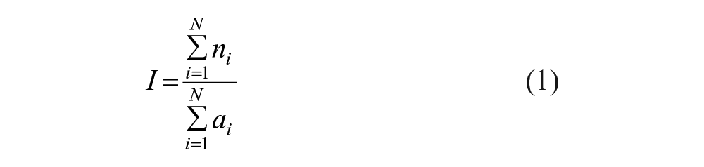
where I is an unbiased estimator of the staining index for the subset, N is the total number of sampled tiles, n_i is the total number of (DAB) positive pixels in the tissue type of interest in the i^th tile, and a_i is the total area of the tissue type of interest in the i^th tile. Then we calculated the 95% confidence intervals of the weighted means of the staining indices from all of the random subsets from all repetitions (100 random subsets) for each treatment arm (Mattfeldt et al. 2013). We then checked for overlaps in the confidence intervals. Non-overlapping 95% confidence intervals denote statistically significant differences between the means of the two groups at the significance level of 0.05 (Schenker and Gentleman 2001).

We performed local LOESS regression with LOESS smoothing parameter (span) set to 0.75 and used second-degree polynomials. We used a significance level of 0.05 for all tests.

Results

Increased Sensitivity of Detection

We compared the sensitivity of statistical inference of both the MWW and NCI tests deriving inputs from of our grid quantification method against whole-slide indices (Fig. 3). The MWW test, based on whole-slide indices, detected significantly higher levels of the CD34 index for placebo than SOC at the end of the study (p<0.05). This difference in CD34 indices is consistent with the known antiangiogenic effects of cyclophosphamide, doxorubicin and etoposide (used in SOC) (Mailloux et al. 2001; Kalyanaraman et al. 2002; Santosuosso et al. 2002; Bruneel et al. 2005; Marklein et al. 2012). The MWW tests based on whole-slide indices do not detect any significant difference in other indices (CASP3, H3 and KI67) between the two arms at the end of study. This lack of difference between the two arms is consistent with the waning cytotoxic effect of the SOC drugs, which had reduced to levels not detectable by MWW tests based on whole-slide indices by the end of the study (see the section phenotypic alterations for a detailed analysis). In contrast, both the MWW and NCI tests deriving inputs from grid quantification detected statistically significant differences in all four staining indices between the two arms at the end of the study. This observation holds true at various tile sizes and samples per draw. Thus, our grid quantification provides a higher sensitivity of detection to the MWW test compared to whole-slide indices. In general, the MWW test shows higher sensitivity of statistical inference, requiring fewer samples per WSI for any given tile size as compared with the NCI test.

Figure 3.

Comparison of probability of significance (statistical power) between Mann-Whitney-Wilcoxon (MWW) tests and non-overlapping confidence intervals (NCIs) at the end of the study (Day 103). Probability of significance for sampled data calculated by portion of MWW tests (out of 100 repeats) with p-values less than 0.05. Difference in staining index between standard of care (SOC) and placebo are significant at level of 0.05 when CIs do not overlap. We use a combination of fill colors and symbols to indicate statistical significance. Solid white patches with gray border indicates no statistically significant difference is detected by MWW and NCI tests. All the combinations of fill colors and symbols in the legend have additive interpretations (e.g., light blue fill with ‘-’ means placebo staining index is statistically greater than SOC in both MWW and NCI tests).

Representation of the Heterogeneity Landscape

Statistical tests using samples from IHC index distributions may lead to unreliable conclusions due to sampling bias. To measure sampling bias at any given tile size, we calculated two types of relative errors for the sample mean and sample variance (Table 1). ${\epsilon }_{M1}$ and ${\epsilon }_{V1}$ represent the extent of bias in sample means and variances; ${\epsilon }_{M2}$ and ${\epsilon }_{V2}$ represent the extent of deviation of sample means and variances from whole-slide means and whole-grid variances, respectively. Figure 4 shows the distribution of errors for tile sizes 50 and 500 µm. Parts A and C of Fig. 4 show that both ${\epsilon }_{M1}$ and ${\epsilon }_{V1}$ are symmetric about zero for any given number of sample tiles per WSI and their spreads shrink rapidly with an increasing number of sample tiles per WSI, for samples from both 50 and 500 µm tile sizes used in the statistical tests (this is true for all tile sizes we tested; data not shown). Similarly, parts B and D of Fig. 4 show that the spreads in both ${\epsilon }_{M2}$ and ${\epsilon }_{V2}$ shrink rapidly, approaching zero, with an increasing number of sample tiles per WSI. These observations show that our sampling did not introduce bias in means and variances for the range of tile sizes tested.

Table 1.

Errors for the Sample Mean and Sample Variance.

	Mean	Variance
Bias	${\epsilon }_{M1}=E\left(\frac{{\mu }_i-\mu }{\mu }\right)$	${\epsilon }_{V1}=E\left(\frac{{\sigma }_i^2-{\sigma }^2}{{\sigma }^2}\right)$
Deviation	${\epsilon }_{M2}=E\left(\frac{\left|{\mu }_i-\mu \right|}{\mu }\right)$	${\epsilon }_{V2}=E\left(\frac{\left|{\sigma }_i^2-{\sigma }^2\right|}{{\sigma }^2}\right)$

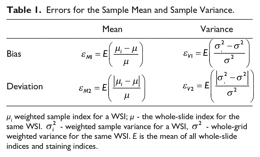
µ_i weighted sample index for a WSI; µ - the whole-slide index for the same WSI. ${\sigma }_i^2$ - weighted sample variance for a WSI, ${\sigma }^2$ - whole-grid weighted variance for the same WSI. E is the mean of all whole-slide indices and staining indices.

Figure 4.

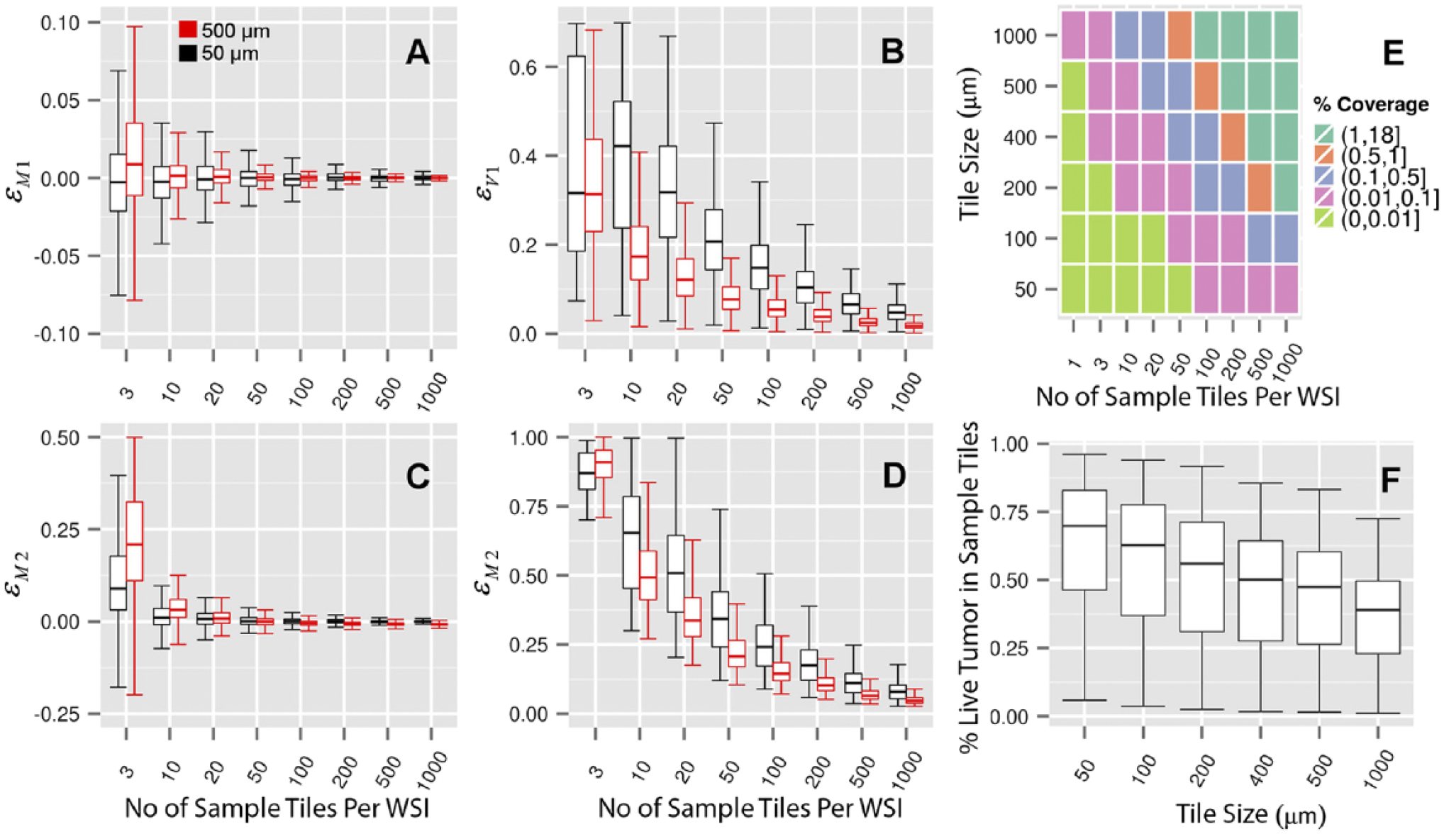
(A–D) Boxplot of errors in sample mean and sample variance per WSI for tile size of 50 µm and 500 µm (all four staining indices combined). (E) Mean sampled viable tumor tissue percentage coverage. Percentage coverage greater than one represents oversampling. (F) Mean percent viable tumor tissue content of sampled tiles. Error bars in the box plots (A–D and F) show the 95% confidence interval. The two hinges correspond to the first and third quartiles. The midline corresponds to the median.

Phenotypic Alterations

We tracked the phenotypic properties over the course of the study to see if significant alterations in phenotypic properties correlated with the timing of SOC treatment. Figure 5 shows the phenotypic alterations as measured by four IHC staining indices over the course of the study. In general, the SOC treatment (cytotoxicity) that ended at day 26 (end of week 1 of course 2) significantly affected the phenotypic properties of tumor cells and tumor blood vessels both during and after the treatment period. The exits of mice from the SOC arm during the course of treatment were due to illness and not tumor burden. CASP3 indices in tumors in the SOC arm harvested during treatment were higher than in tumors in the placebo arm from the same period. The magnitude of this difference gradually decreased over time and reached its lowest at the end of the study. Initially, H3 and Ki67 indices were higher in the placebo arm. These indices for the SOC arm quickly reached levels similar to the placebo arm by around day 42 and became higher for the SOC arm past day 42 and remained so for the rest of the study. The CD34 index of the SOC arm widely fluctuated during the early part of the study and decreased to lower levels than that of the placebo arm by day 50, and remained so for the rest of the study.

Figure 5.

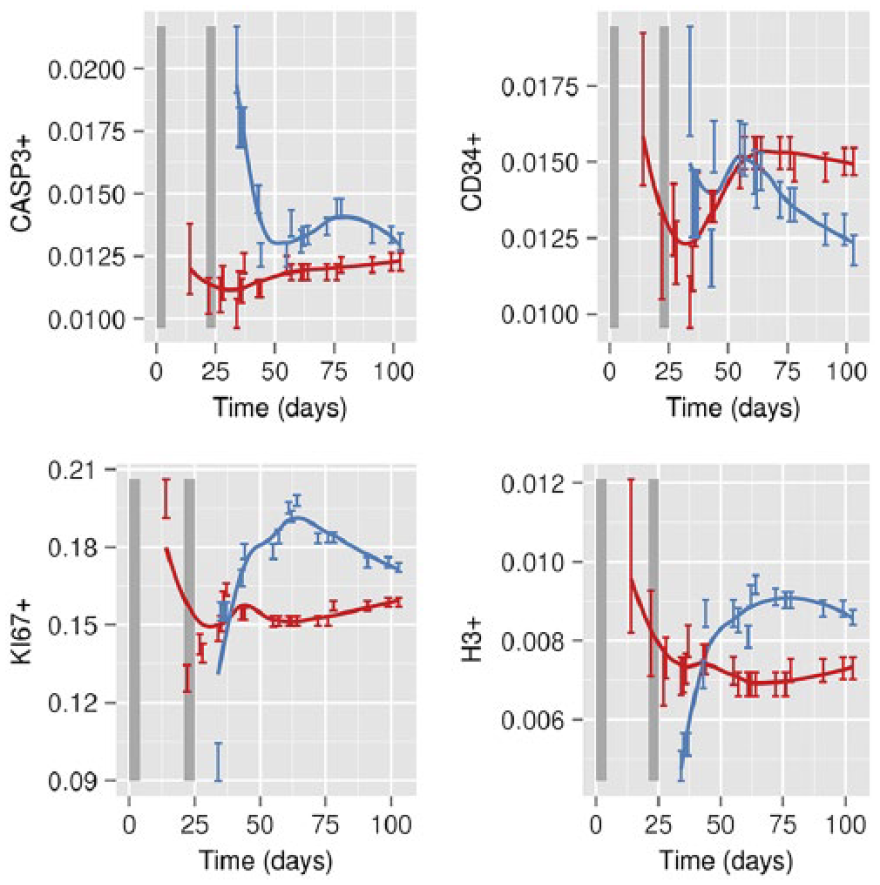
Phenotypic (IHC staining index) alterations over time using LOESS regression on whole-slide indices. Blue represents standard of care (SOC); red, Placebo. Error bars represent 95% confidence interval (CI), estimated using 100 sample tiles of size 200 µm × 200 µm per image. Vertical shaded areas represent the days of treatment during Course 1 (days 1 to 5) and Course 2 (days 22 to 26).

Phenotypic Alterations – Statistical Analysis

We compared the sensitivity of statistical inferences of both the MWW and NCI tests (where appropriate) resulting from inputs from three staining index calculation methods: 1) whole-slide index, 2) non-overlapping whole-grid indices, and 3) our method of repeated uniform random sampling of non-overlapping whole-grid tiles (Fig. 6). Since the temporal analysis adds a third dimension, a full detailed comparison of all of the tile sizes and sample sizes in Fig. 3 is prohibitively long. Without a loss of generality, we focus on two tile sizes for IHC quantification, as representatives of local cellular activity (50 µm) and tissue scale activity (500 µm). The results of this comparison in Fig. 6 show the increased detection sensitivity of the MWW test deriving inputs from our quantification method, made obvious by the absence of significance in the MWW test deriving inputs from the whole-slide at different time points. In general, if the MWW tests detect significant differences in either direction using whole-slide indices as input, then both MWW and NCI tests detect significant differences in the same direction, using inputs from our quantification method. Also, the MWW tests deriving inputs from our method required a fewer number of samples to detect significant differences as compared with the NCI tests for a given tile size and generally in agreement with the direction of statistical significance using whole-slide indices, if present. Whereas these observations are also mostly true for comparisons between the directions of significance of the MWW method based on inputs from our method and that of the whole-grid, there are a few exceptions, which are discussed in detail in the Supplemental Material.

Figure 6.

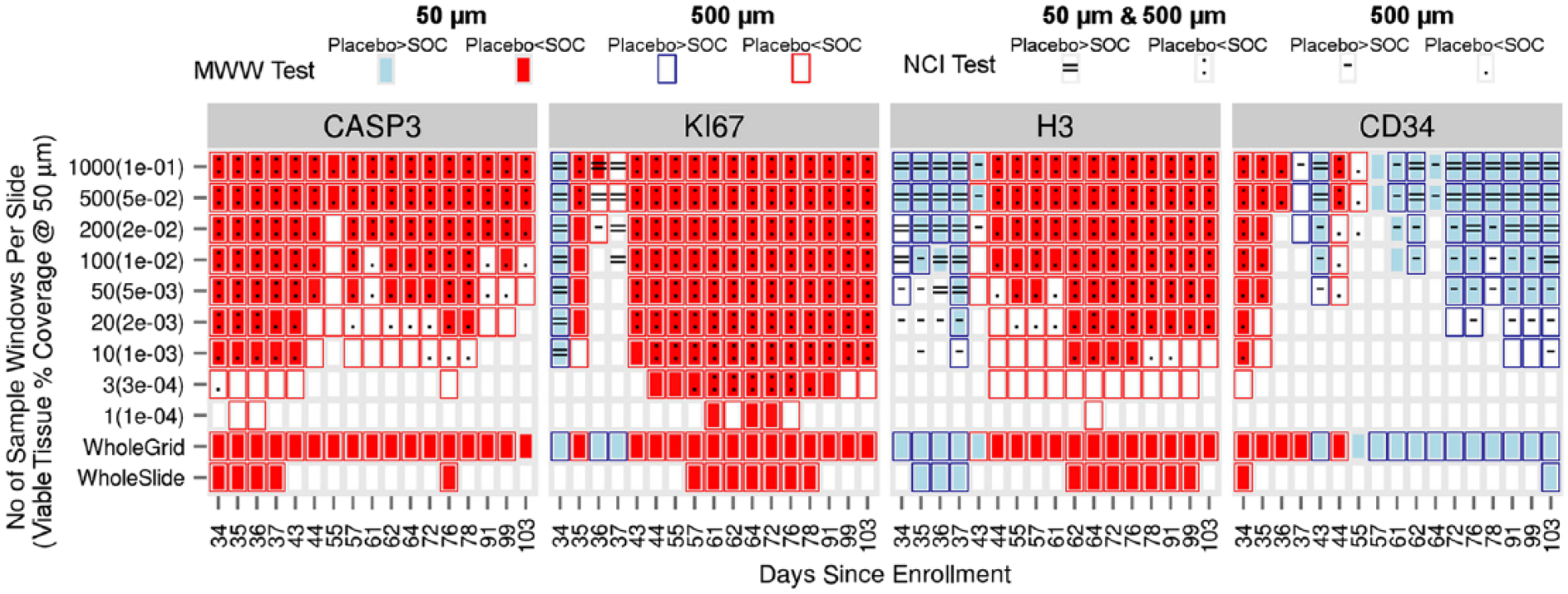
Heat map of significance for two one-sided Mann-Whitney-Wilcoxon (MWW) tests and non-overlapping confidence interval (NCI) tests (tile size of 50 µm and 500 µm) at the significance level of 0.05. We calculated the significance of the MWW tests for the sampled data as the fraction of the tests that reached significance less than 0.05 for more than 95% of the repeats (total of 100 repeats). We used the entire grid data without sampling in MWW tests to calculate a p-value for whole-grid tests. We used whole-slide index in MWW tests to calculate a p-value for whole-slide tests. We used a combination of fill and border colors and symbols to indicate statistical significance. Solid white patches with gray border indicates no statistically significant difference is detected by MWW and NCI tests. All the combinations of fill and border colors and symbols in the legend have additive interpretations (e.g., light blue fill with dark blue border with ‘=’ means placebo staining index is statistically greater than SOC at 50 µm and 500 µm tile sizes in both MWW and NCI tests).

Discussion

With the advent of WSI analysis tools, the field of digital pathology has gained prominence in recent years as a potential solution to minimizing subjectivity in IHC quantification by including entire histological sections. It is an established fact that tumors exhibit spatial heterogeneity. Existing WSI analysis tools do not account for this spatial heterogeneity. Therefore, information is lost when the heterogeneity is reduced into a single IHC index per slide.

Our method captures the underlying spatial heterogeneity in WSIs by calculating distributions of staining indices. It uses these distributions to reliably compare biological properties of tissue response to therapy. The use of appropriate weights makes our method robust for analyzing fragmented tissues (e.g., viable tumor regions in Fig. 1) because it is not sensitive to partially filled grid tiles. This capability is important for comparing primary tumors to micro-metastases where tumor cells are dispersed across the host tissue in small clusters.

Tests using whole-slide data allow only a single statistical test and provide one p-value, but a single test does not show how sensitive these detected differences are to uncontrolled experimental variations (e.g., the amount of tissue harvested or size of tissue section). To overcome this issue, we sample a fraction of the WSI for each statistical test, and repeat the test. We use percentage coverage of samples used in the tests as a measure of oversampling. We use errors in sample means and variances and percentage coverage as measures of quality of samples. Generally, larger sample sizes have smaller errors in sample means and variances, but they suffer from oversampling and are more likely to artificially deflate the p-values than smaller sample sizes. We regard statistically significant differences detected using a smaller fraction of tissue and smaller errors in sample means and sample variances as more reliable. In our study, for a given tissue percentage coverage (as low as 2%), the choice of tile size of 50 µm provided the lowest level of error and bias and outperformed the tests based on whole-slide index.

In general, (chromogen- and fluorescence-based) IHC is a qualitative or semi-quantitative measure in most applications (Taylor and Levenson 2006; Dunstan et al. 2011). IHC variability (tissue preparation, staining validation, interpretation, lack of standards for 1+, 2+, 3+ positivity) is the major obstacle for a measure to become a quantitative one by use of image analysis and is a challenge for the development of new biomarkers (Dunstan et al. 2011). However, under standardized conditions, IHC staining intensities have been used to accurately quantify protein expressions and validated against gold-standard techniques (Matkowskyj et al. 2003). There have been advancements toward the standardization of IHC (Taylor and Levenson 2006; Dunstan et al. 2011; Pantanowitz et al. 2013). Our method can be used with both chromogen- and fluorescence-based IHC. Higher detection powers by our weighted grid method, coupled with standardized IHC practices, may significantly improve the predictive power of current diagnostic and prognostic assays, and allow for exploring novel assays.