Assessing Cortical Thickness in Human Tibiae With Sonography vs Computed Tomography: A Pilot Study

Abstract

Osteoporosis is a public health problem worldwide that decreases bone strength and increases the risk for fractures. Cortical thickness of long bones has gained attention because of its contributions to the resistance of bone fracture. What is currently lacking is a nonionizing imaging modality that assesses cortical bones with a sensitivity equal to that of computed tomography (CT). Tibiae were utilized to compare cortical thickness measurements recorded with diagnostic medical sonography (DMS) and CT. Four percentage sites (4%, 38%, 50%, 66%) were identified along the tibiae, and cortical measurements were taken from 3 views (anterior, medial, lateral). Medial views at all sites except 38% had DMS full measurements that were not significantly different than those collected with CT. The 4% sites in all views yielded the most cortical thickness measurements that were not significantly different from those of CT. These promising results at DMS full 4% sites open the possibility of translating this methodology to bones that have thin cortices and high risks of fragility fractures, such as the radius.

Approximately 200 million people worldwide have osteoporosis, a disease that contributes to about 9 million fragility fractures every year. ¹ This accounts for $20 billion in health care costs in the United States alone. ² Most bones are composed of two main compartments: the trabecular bone, known as spongy bone, and the cortical bone, which is a compact bone that forms the outer shell around the trabecular bone. With age, skeletal fragility becomes more prevalent as some individuals experience bone loss and microstructural deterioration in both the trabecular and cortical compartments. This increase in fragility, with an increased risk of falling, causes persons of advanced age to be more susceptible to bone fractures. ² Fracture risk grows exponentially with the presence of bone disease, such as osteoporosis. Osteoporosis is characterized by low bone mineral density (BMD) and by changes in the microstructure of the bones, thus resulting in a decrease in bone strength and an increased risk for fractures. ² This issue will continue to escalate as life expectancy increases and the aging population grows, resulting in an even greater economic burden in health care costs. ³

Clinically, areal BMD obtained by dual-energy x-ray absorptiometry has been the gold standard in determining bone strength for the diagnosis of osteoporosis. ² Yet, <50% of the changes that affect whole-bone strength are directly caused by variations in BMD.^4,5 According to criteria of the World Health Organization, osteoporosis is determined if the areal BMD value obtained is ≥2.5 SD below the young adult reference mean (T score ≤ −2.5 SD). ⁶ However, multiple studies revealed that fragility fractures occur in patients with T scores > −2.5.^4,5,7 A prospective study consisting of 7806 participants aged >55 years found that 56% and 79% of fractures that occurred in women and men, respectively, had T scores between −1.0 and −2.5. ⁵ Nonetheless, merely lowering the T-score threshold is not a solution. Bringing the T-score threshold closer to zero will also decrease the threshold value for intervention, resulting in the treatment of a largely low-risk population and severely increasing health care costs. Despite a noted relationship between density (areal BMD) and osteoporosis, there are density-independent changes (e.g., bone geometry and quality) that dual-energy x-ray absorptiometry fails to account for when evaluating bone.

Historically, fragility fractures were believed to be a direct result of trabecular bone loss. Yet, while bone loss in the cortical compartment occurs more slowly than in the trabecular compartment, cortical bone accounts for 70% of all appendicular bone loss with increasing age. ⁸ During puberty, cortical bones become thicker because bone formation on the periosteal surface occurs at a much higher rate than resorption on the endocortical surface. Conversely, during adulthood, there can be a net loss of bone because endosteal resorption occurs at a faster rate than periosteal apposition. The reduced rate of periosteal apposition of the cortex leads to a change in the size and contour of the bone and is a main contributor to the loss of cortical thickness. ⁹

Multiple studies found that elderly individuals have lower cortical thickness and significantly higher cortical porosity than do their younger counterparts. Kazakia and colleagues’ analysis of the tibia revealed a 181% increase in cortical porosity (P < .001) and a 12% decrease in cortical thickness (P < .001) among elderly subjects versus young adults. ¹⁰ The increase in cortical porosity and decrease in cortical thickness greatly affect the strength of the bone. Further research focused on evaluating the mechanical properties of bone found that a 20% reduction in the periosteal surface of the cortex led to a 120% increase in strain energy density; yet, thinning in the trabeculae compartment by 20% resulted in a less pronounced increase of 37% in strain energy density. ¹¹ Given the importance of assessing cortical and trabecular bone compartments, there has been a growing interest in identifying an imaging modality that can evaluate the contribution of cortical bone to skeletal fragility.

High-resolution peripheral quantitative computed tomography (HR-pQCT) is an in vivo imaging technique that is capable of visualizing the separate compartments within bone and assessing the microstructure within each compartment. HR-pQCT is able to detect changes that occur between pre- and postmenopausal females. Boutroy and colleagues found that HR-pQCT was able to detect a 28% to 41% (P < .001) decrease in cortical thickness, in addition to an 8% to 19% (P < .001) decrease in trabecular thickness. ¹² Although HR-pQCT is capable of distinguishing and evaluating cortical bone, it is typically used in research settings, given its high cost and low availability. ⁶

Furthermore, with a greater awareness to minimize patient exposure to ionizing radiation in health care organizations, especially pediatrics, a nonionizing modality should be explored. Diagnostic medical sonography (DMS) uses reflected acoustic pressure waves (ultrasound) to produce an image of internal structures. Major benefits to this modality include the lack of ionizing radiation, wide accessibility, and cost-effieciency. ⁶ While it is widely believed that DMS is incapable of evaluating adult bones, studies demonstrated the effectiveness of DMS in evaluating the surface of the cortical bone for fractures. ¹³ The discovery that DMS can evaluate the surface of the cortical bone for fractures opens the possibility for further research in quantifying the thickness of cortical bone—an important indicator of bone strength.

Therefore, the purpose of this preliminary study was to investigate the feasibility of DMS in measuring the cortical bone thickness of the tibia. The tibia was selected for cortical thickness evaluations because of the repeated fatigue that it endures as a weight-bearing bone. Thus, we decided to utilize the tibia to compare the cortical thickness measurements recorded with DMS with those measured with clinical computed tomography (CT). Despite the clinical impetus to use nonionizing imaging modalities, there is a known acoustic impedance difference between bone and soft tissue that may pose a challenge when bones are imaged with DMS. Therefore, we hypothesized that there would be a difference in the cortical bone thickness measurements between DMS and CT.

Method

Subjects

A preclinical research approach was used to evaluate a cohort of four postmortem human subjects (PMHSs; n = 8 lower extremities) donated to The Ohio State University Body Donor Program. The sample consisted of one man and three women with a mean ± SD age of 62.8 ± 16.6 years, height of 169.6 ± 13.1 cm, and body mass of 57.6 ± 16.0 kg. All PMHSs were fresh (not embalmed) and frozen to −20°C until the time of imaging, at which point they were thawed to room temperature before imaging with DMS. Afterward, the tibiae were excised and wrapped in saline-soaked gauze, then frozen at −20°C until CT imaging.

Because of accessibility, clinical CT was used rather than HR-pQCT. However, performing the CT on ex vivo tibiae of PMHSs allowed the research team to obtain high-resolution images on which cortical thickness measurements could also be obtained.

Diagnostic Medical Sonography

The research team utilized a GE Logiq i machine and a 12-MHz linear transducer to obtain images of the tibiae. The GE Logiq i machine was set at a high frequency (12 MHz) to acquire a high spatial resolution image. Quality control testing of the equipment was performed with use of a tissue-mimicking phantom on a monthly basis, and data revealed a difference of <0.05 mm for axial resolution and <0.17 mm for lateral resolution.

After the PMHSs were prepared for DMS imaging, the tibiae were palpated, and tibial length was determined by measuring from the medial malleolus to the medial tibial plateau. Tibial length was used to identify measurement sites at 4%, 38%, 50%, and 66%, with the medial malleolus set as 0% (Figure 1). The measurement sites were then marked on the skin of the PMHSs. These specific measurement sites were selected to coincide with anatomic sites that were used in other published studies, allowing for the results to be compared with the literature. ¹⁴

Figure 1.

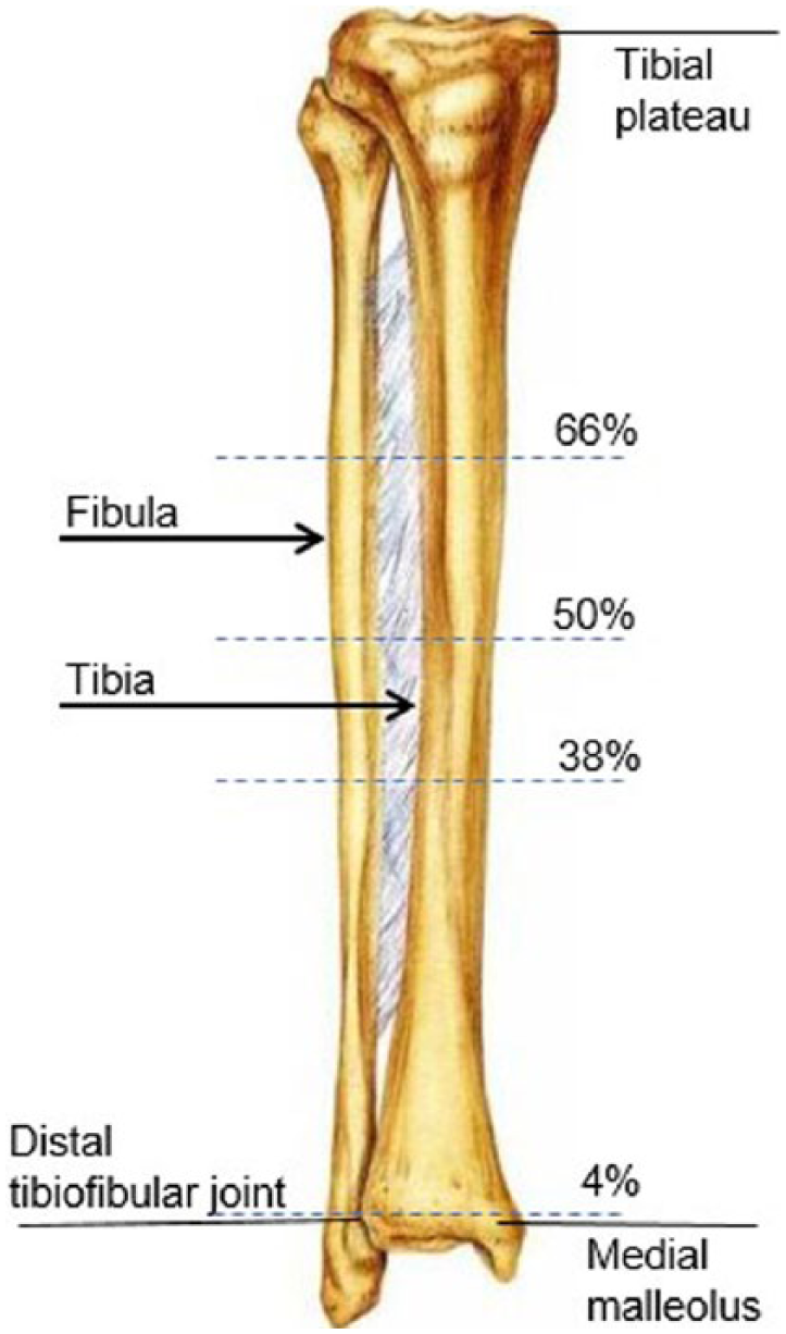
Measurement sites for right tibia. 0% = distal tip of the medial malleolus.

Three views were taken with DMS at each measurement site to represent the anterior, medial, and lateral cortical thicknesses of each tibiae. As the cortical bone in the tibiae endure fatigue from repeated loading, the damage to the cortex varies depending on the magnitude and location, thus resulting in a heterogeneous cortical thickness. ¹⁵ Therefore, it was imperative to take images at different sites and varied transducer positions to capture the variation in cortical thickness measurements.

During imaging with DMS, the anterior crest was used as a landmark for all anterior views at the 38%, 50% and 66% sites. At the 4% site, however, the anterior crest does not exist; therefore, the anterior view was taken approximately at the center of the anterior tibia. To obtain the medial view, the transducer was moved 90° from the anterior location toward the medial side of the leg. To obtain the lateral view, the transducer was moved 90° from the anterior location toward the lateral side of the leg. The overall gain and depth varied among images to optimize visualization.

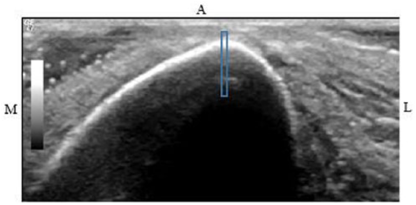
After the images were obtained, a narrowed region of interest (ROI) was established for each view to determine where the measurements would be taken. The ROIs at the 38%, 50%, and 66% sites for the anterior images were set at the anterior crest (Figure 2). At the 4% site, a measurement was taken between the ends of the cortical surface visualized on either side of the image. At the midpoint of this measurement, a perpendicular line was drawn toward the cortex and set as the ROI (Figure 3). Based on the assumption that the sonographer moved the transducer 90° from the anterior ROI to the medial or lateral side of the tibia, the ROI was set by measuring the distance between the ends of cortical surface visualized on either side of the screen and by drawing a perpendicular line from the midpoint of this measurement up toward the cortex.

Figure 2.

Sonographic image of the left tibia at anterior 38%. Anterior region of interest (blue box) set at the anterior crest.

Figure 3.

Sonographic image of the left tibia at anterior 4%. The midpoint between the visualized cortical ends was determined, and a perpendicular line was drawn toward the cortex (solid pink lines), which was utilized to set the anterior region of interest (blue box).

Since the true depth of penetration that ultrasonic pressure waves can travel through a cortical bone is unknown, two sets of measurements were taken at each ROI. It was assumed that the highly reflective surface of the tibia bone was the cortical bone. Therefore, the first set of measurements were labeled “border” and contained the depth of the brightest pixels visualized (Figure 4A). Yet, it was not apparent how much of the cortical bone was detected below the highly reflective surface, as opposed to what might be artifact. Therefore, the second set of measurements were labeled “full” and contained the maximum depth of pixels visualized that were believed to be the cortex (Figure 4B).

Figure 4.

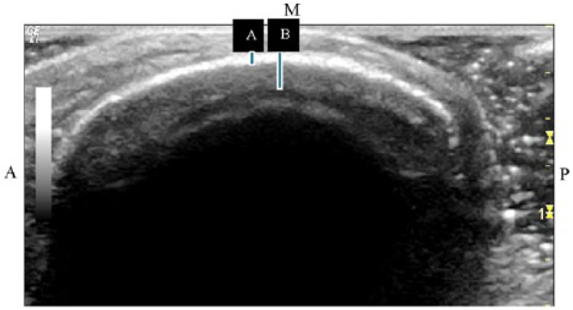
Sonographic image of left tibia at medial 50%: (A) border measurement; (B) full measurement.

ImageJ (v 1.51k; National Institutes of Health) was utilized for measuring all cortical thicknesses for DMS. It was crucial to set the scale before measuring with it. Having varying depths with DMS changed the number of pixels in the image. Therefore, the scale had to be adjusted for each image, depending on the depth (Table 1). Five measurements were collected for each established ROI for the “border” and “full” data sets. The highest and lowest measurements of the five values were excluded, and the remaining three values were averaged and used for further analysis.

Table 1.

Depth Scale Settings for Diagnostic Medical Sonography Measurements.

Image Depth, mm	Pixels/mm
20	24.200
25	19.400
30	16.200
35	13.887

Computed Tomography

The research team utilized the clinical Philips Vereos Digital 64-Slice Ingenuity CT, located at the Wright Center of Innovation in Biomedical Imaging, to obtain images of the ex vivo tibia at 0.335-mm resolution. The algorithm was changed from the standard algorithm used to image soft tissue to a bone algorithm to increase the sharpness of the bony detail.

The true length of the tibia was measured from the distal medial malleolus to the tibial plateau, similar to the palpitation method employed prior for DMS imaging. Axial or cross-sectional slices (0.671 mm in thickness) of the tibia were taken at the same levels as with DMS (4%, 38%, 50%, and 66% of total tibial length, with 0% representing the distal tip of the medial malleolus) with OsiriX MD (v 8.0.1). Additionally, three views (anterior, medial, and lateral) were analyzed from each image obtained at the sites.

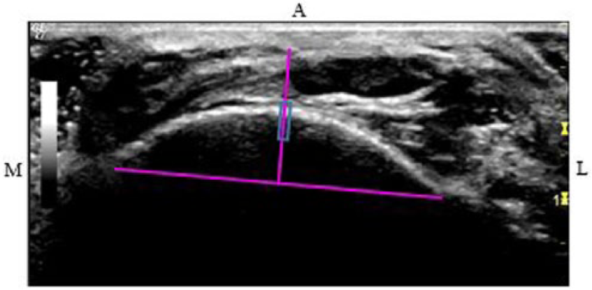
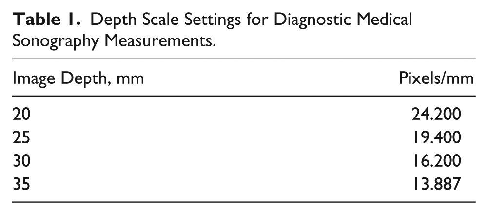
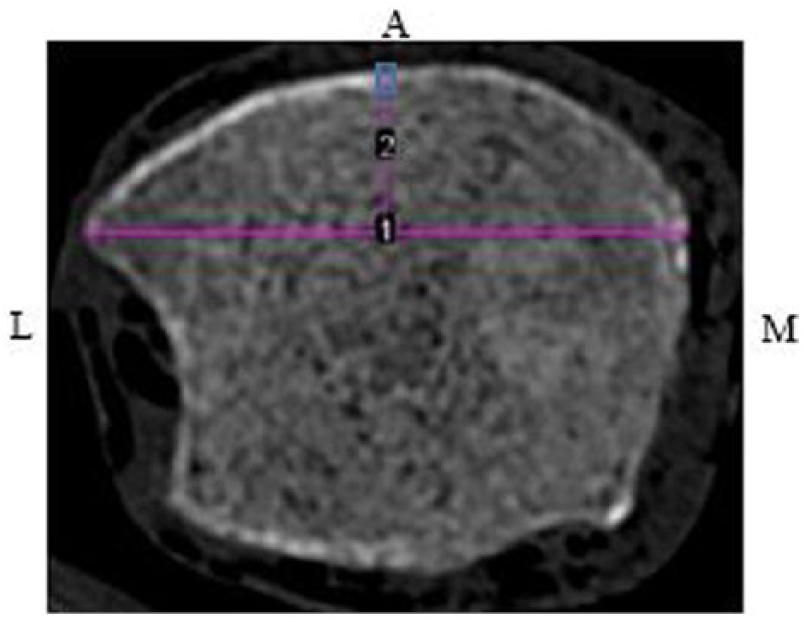
An ROI was established for each view. The anterior crest was set as the ROI for the anterior views of the tibiae at 38%, 50%, and 66%. Unlike with DMS, at the anterior 4% site, the medial malleolus and distal fibular notch are visualized; therefore, a measurement was taken between the points. At the midpoint of this measurement, a line was drawn toward the cortex and set as the ROI (Figure 5). To determine the ROI for the lateral and medial views of the tibiae at all sites, a line was drawn from the anterior ROI down to the posterior border of the tibia. From the midpoint of this measurement, a perpendicular line was drawn across the cross-sectional tibia (Figure 6). The lateral and medial ROIs were consistently set at 90° from the anterior ROI.

Figure 5.

Computed tomographic image of left tibia at anterior 4%. Midpoint level of the measured distance from the medial malleolus to the distal fibular notch (1) was utilized to set the anterior region of interest (blue box) at 4%.

Figure 6.

Computed tomographic image of the left tibia at 38%. Midpoint level of the measured distance from the anterior region of interest to the outer posterior cortex (1) was utilized to determine the level for the medial (2) and lateral (3) regions of interest.

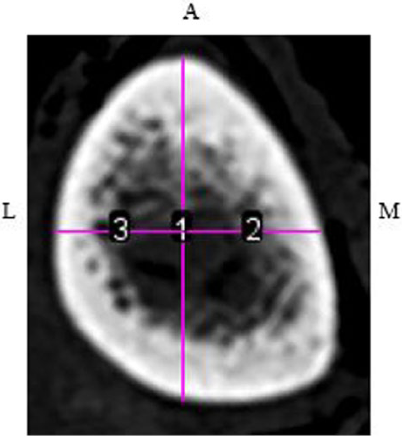
In measuring the cortical thickness with CT, the brightest pixel depth was measured (Figure 7). The light gray pixels represent what once was cortical bone that went through endosteal resorption; thus, these pixels were excluded from the measurement. ⁹

Figure 7.

Computed tomographic image of the left tibia at 38%. Anterior and lateral cortical thickness measurements (solid pink lines) within the regions of interest (blue boxes).

ImageJ was utilized for measuring all cortical thicknesses for CT. The scale was set at 6.015 pixels/mm for all images. Five measurements were collected at each established ROI. The highest and lowest measurements were excluded from each ROI. The remaining three values were averaged and used for further analysis.

Statistics

Of the 864 possible measurements, 840 were utilized for analysis based on optimal image quality. In some locations, the cortical layer was not visualized clearly at the specified ROI, possibly because of endosteal resorption, and was thus excluded from the data. Additionally, since the data did not follow the assumption of a normal distribution, the data points were analyzed with Minitab (v 17) via the Wilcoxon signed rank test. Cortical thicknesses measured for DMS border and DMS full were compared with each other and with measurements collected from CT. The alpha level was set to 0.05 a priori. CT was set as a reference for DMS full and DMS border measurements.

Results

Descriptive Statistics

Table 2 displays the descriptive data obtained from the Wilcoxon signed rank test. The median values clearly demonstrate that the DMS border measurements yielded the lowest measurements, the CT measurements yielded the largest measurements, and the DMS full measurement values fell between DMS border and CT. It was also clear that DMS full and DMS border measurements were significantly different from each other at all sites and views (P < .01).

Table 2.

Descriptive Statistics for Cortical Thickness (mm) Measurements Made With DMS and CT at the Four Measurement Sites and Three Image Views.

Site: View	DMS Full			DMS Border			CT
	n	Median	IQR	n	Median	IQR	n	Median	IQR
4%
Anterior	7	0.523	0.234	7	0.453	0.100	8	0.558	0.302
Medial	7	1.082	1.031	7	0.336	0.210	7	0.471	0.222
Lateral	8	0.668	0.261	8	0.481	0.158	7	0.720	0.641
38%
Anterior	8	2.267	0.927	8	0.548	0.331	8	6.570	5.910
Medial	8	2.082	1.792	8	0.437	0.234	8	2.839	1.162
Lateral	7	1.144	1.156	7	0.358	0.253	8	2.454	2.293
50%
Anterior	8	1.438	1.684	8	0.595	0.331	8	8.230	7.650
Medial	8	2.410	1.147	8	0.467	0.215	8	2.705	1.748
Lateral	8	1.144	0.660	8	0.479	0.283	8	3.031	1.395
66%
Anterior	8	1.720	1.628	8	0.586	0.284	8	7.110	5.910
Medial	8	2.064	1.685	8	0.417	0.256	8	2.690	1.539
Lateral	8	1.003	0.312	8	0.536	0.287	8	2.091	0.793

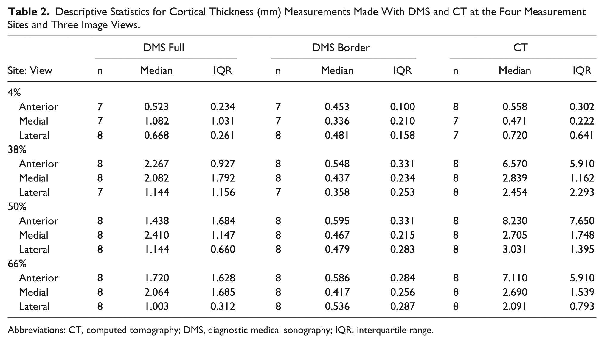
Abbreviations: CT, computed tomography; DMS, diagnostic medical sonography; IQR, interquartile range.

DMS Border vs CT

At the 4% site, the medial view measurements were significantly different than those collected from CT (P < .04). However, the measurements collected from the anterior and lateral views were not significantly different from the CT measurements (P < .05 and P < .35, respectively). At the 38%, 50%, and 66% sites, the measurements collected from all views were significantly lower than the CT values (Table 3).

Table 3.

Median Differences From Wilcoxon Signed Rank Test for the DMS Border vs CT Thicknesses (mm).

Site: View	DMS Border vs CT
	n	Median Difference	IQR	95% CI	P Value a
4%
Anterior	7	0.129	0.275	3.520 to 6.300	.05
Medial	7	0.065	0.091	0.029 to 0.150	.04
Lateral	7	0.124	0.777	−0.215 to 0.562	.35
38%
Anterior	8	6.090	5.640	4.390 to 9.210	.01
Medial	8	2.324	1.103	1.800 to 3.260	.01
Lateral	7	2.393	2.984	1.300 to 4.650	.04
50%
Anterior	8	7.520	7.320	4.910 to 11.370	.01
Medial	8	2.284	1.608	1.290 to 3.310	.01
Lateral	8	2.320	1.299	1.460 to 2.890	.01
66%
Anterior	8	6.470	6.230	4.600 to 9.380	.01
Medial	8	2.110	1.300	1.360 to 2.640	.01
Lateral	8	1.422	0.726	0.964 to 1.857	.01

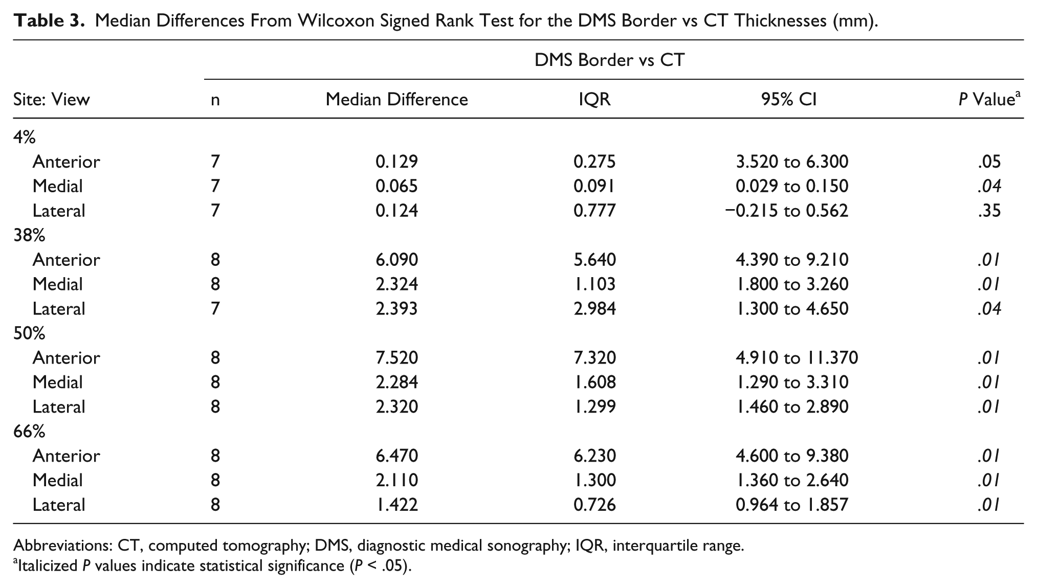
Abbreviations: CT, computed tomography; DMS, diagnostic medical sonography; IQR, interquartile range.

a

Italicized P values indicate statistical significance (P < .05).

DMS Full vs CT

At the 4% site, the measurements collected from the anterior view were not significantly different from those of CT (P < .67). The measurements collected from the medial and lateral views were also not significantly different from the CT values (P < .06 and P < .55; Table 4). Similar to those of the DMS border, measurements from all views (anterior, medial, and lateral) at the 38% site were significantly lower than those collected from CT (P < .04, P < .03, and P < .04; Figure 8). Additionally, the anterior and lateral view measurements at the 50% and 66% sites were significantly lower than the CT measurements. However, the medial view measurements for the 50% and 66% sites were not significantly different from the CT values (P < .44 and P < .23; Figure 9).

Table 4.

Median Differences From Wilcoxon Signed Rank Test for the DMS Full vs CT Thicknesses (mm).

	DMS Full vs CT
	n	Median Difference	IQR	95% CI	P Value a
4%
Anterior	7	−0.074	0.281	−0.170 to 0.217	.67
Medial	7	−0.639	0.641	−1.010 to −0.166	.06
Lateral	7	−0.219	0.599	−0.567 to 0.292	.55
38%
Anterior	8	4.490	5.380	3.150 to 7.470	.01
Medial	8	0.461	0.999	0.059 to 0.983	.03
Lateral	7	1.418	3.015	0.700 to 4.220	.04
50%
Anterior	8	5.650	6.540	3.990 to 1.070	.01
Medial	8	0.127	1.227	−0.250 to 1.080	.44
Lateral	8	1.626	1.660	0.470 to 2.270	.03
66%
Anterior	8	4.890	4.131	4.000 to 7.490	.01
Medial	8	0.237	0.631	−0.980 to 1.270	.23
Lateral	8	1.040	1.527	0.300 to 1.540	.04

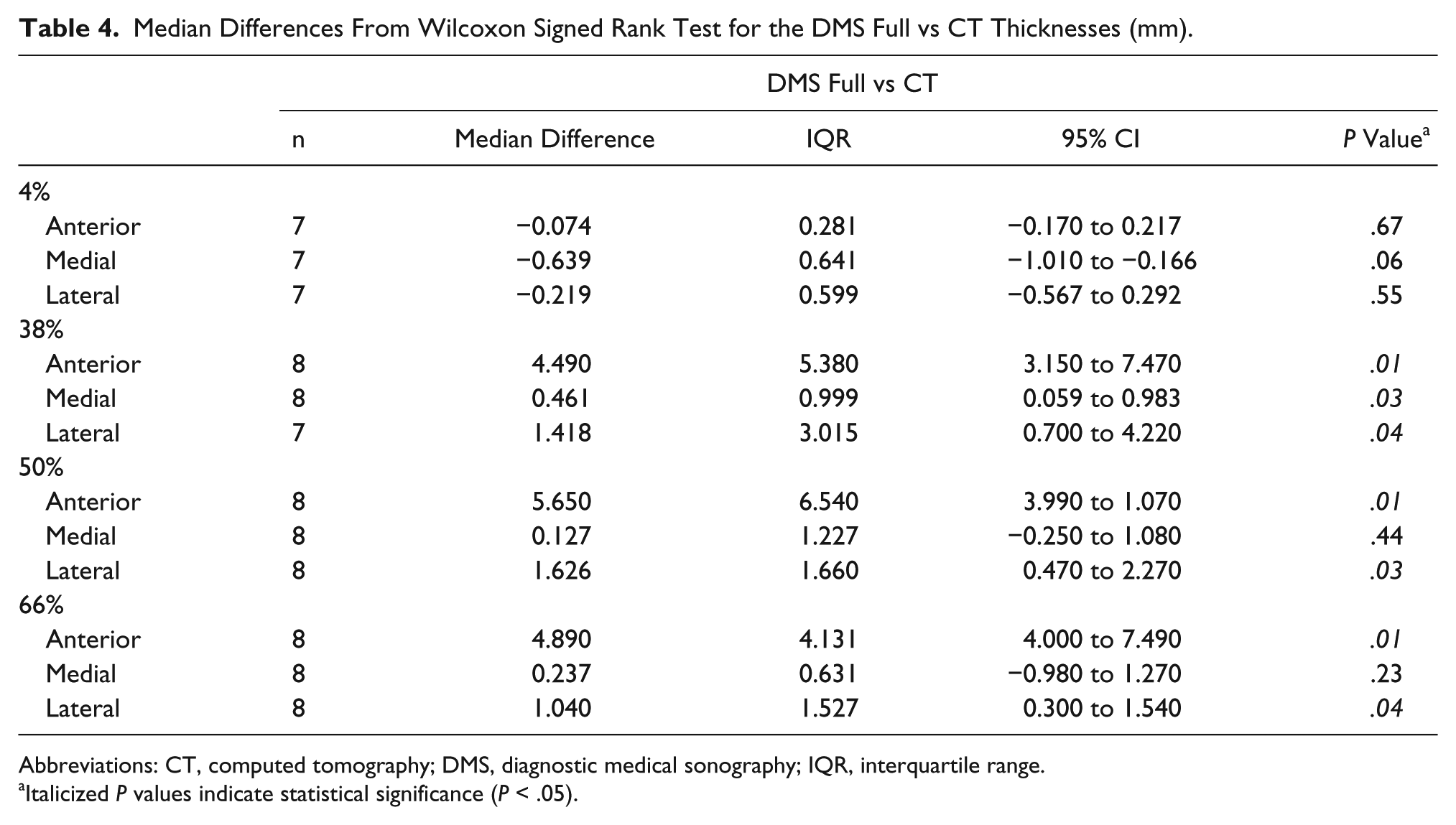
Abbreviations: CT, computed tomography; DMS, diagnostic medical sonography; IQR, interquartile range.

a

Italicized P values indicate statistical significance (P < .05).

Figure 8.

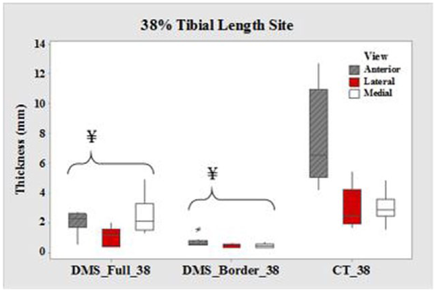
Boxplots of cortical thickness at the 38% tibial length site for all three views. CT, computed tomography; DMS, diagnostic medical sonography. ^¥DMS measurements are significantly different from CT (P < .05). Values are presented as median, interquartile range, and 95% CI.

Figure 9.

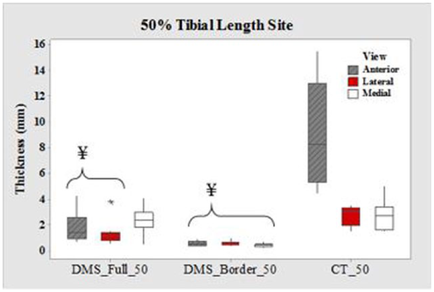
Boxplots of cortical thickness at the 50% tibial length site for all three views. CT, computed tomography; DMS, diagnostic medical sonography. ^¥DMS measurements are significantly different from CT (P < .05). Values are presented as median, interquartile range, and 95% CI.

Discussion

As expected, the DMS border measurements consistently yielded significantly lower values than those of CT in all views at the 38%, 50%, and 66% sites. When only the depth of the brightest pixels visualized was measured, a large portion of what we believe to be cortical bone was omitted. The cortical bone at the 4% site, however, is much thinner and could be why the anterior and lateral DMS border measurements were not significantly different from those of CT.

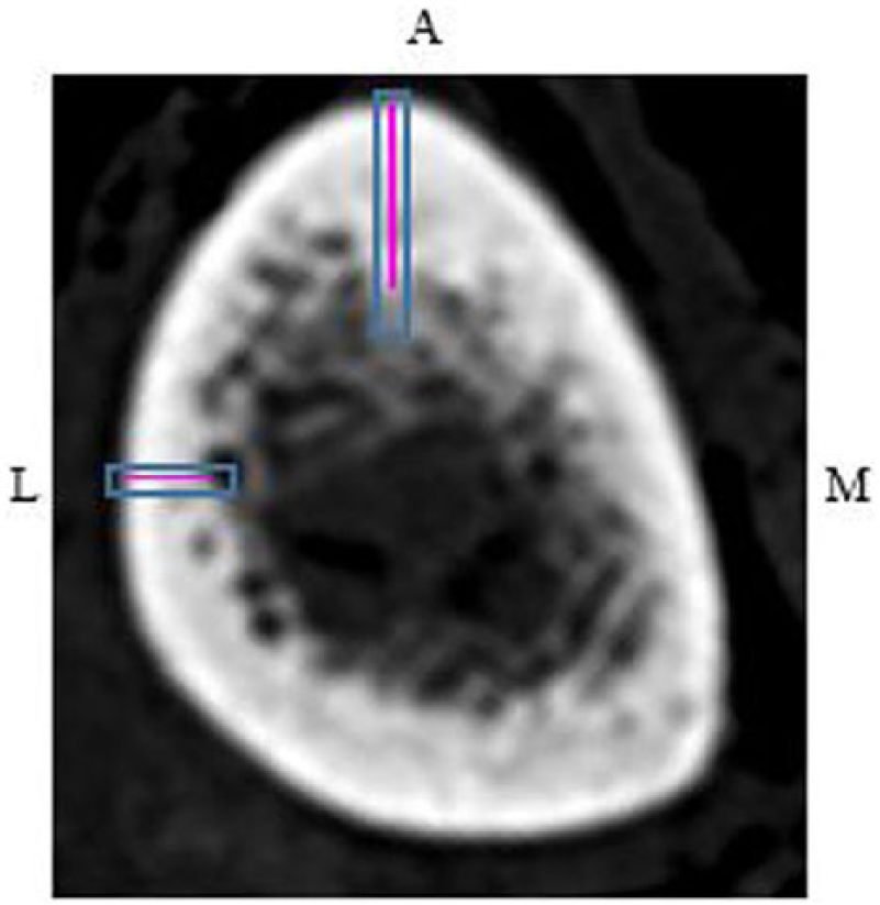
The anterior portion of the bones at the 38%, 50%, and 66% sites were typically thicker than at the medial and lateral portions. The ultrasound pressure waves were likely unable to penetrate through the thick cortices in their entirety, thus resulting in the anterior DMS full measurements at the 38%, 50%, and 66% sites being significantly lower than those from CT. Furthermore, the lateral view measurements at these sites were also significantly different when compared to CT. It was difficult to obtain images where the lateral tibia was directly perpendicular to the ultrasound beam because of the adjacent fibula and muscles (Figure 10). When a structure is approximately perpendicular to the ultrasound beam, more sound waves will be reflected back to the transducer, resulting in a higher-quality image. However, when the structure is approximately parallel to the transducer, as seen with the lateral bone, fewer sound waves return to the transducer, resulting in a “blurry” image of the bone. ¹⁶ Perhaps if a small footprint transducer is utilized, the transducer would fit between the tibia and fibula and be able to produce an image with the tibia perpendicular to the ultrasound beam.

Figure 10.

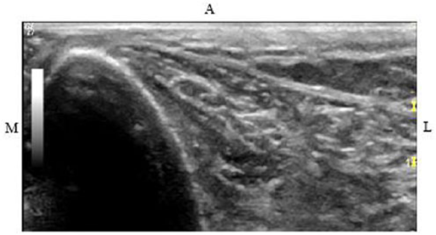
Sonographic image of left tibia at lateral 38%.

It was hypothesized that there would be a difference in the cortical thickness measurements between DMS and CT because of the known difference between the acoustic impedance values of soft tissue and bone. Acoustic impedance depends on the density of the structure and the speed of the sound waves as they travel through the structure. The acoustic impedance is approximately 7.8 × 10⁶ in bone and 1.34 × 10⁶ in soft tissue. As the acoustic impedance difference between interphases increases, the amount of reflection at that surface also increases. ¹⁷ As a result of the large acoustic impedance difference between soft tissue and bone, fewer acoustic pressure waves continue past the cortical surface and instead reflect back to the transducer to be converted into an image. Furthermore, the majority of ultrasound machines are set to assume that the speed of sound is that of soft tissue (1540 m/s); however, this poses a challenge in trying to image bone, which has a speed of sound of approximately 4080 m/s. ¹⁸

Despite these potential limitations in methodology, the medial views at all sites, except 38%, had DMS full measurements that were not significantly different from the measurements collected with CT. Unlike with the lateral views, the medial views of the tibia were obtained with it directly perpendicular to the ultrasound beam. Therefore, the transducer may have been able to detect the low-level signals returning from beyond the cortical surface of the bone. Yet, it is unclear why the medial DMS full measurement at 38% did not follow this same pattern as the other sites.

Of all the sites, the 4% site yielded the most measurements (DMS full) throughout all views that were not significantly different from CT. The cortices are thinnest at the 4% sites, and there was only a small layer of skin separating the transducer from the tibia. With the combination of these two factors, it is possible that the sound waves were able to penetrate through the thin cortices in their entirety.

Limitations

This research study had several limitations. There was a small sample size, which largely consisted of Caucasian women of postmenopausal age. Limitations are also attributed to the body habitus of the PMHSs. When edema was present, DMS images were very limited because of the increase in sound absorption; thus, fewer reflections returned to the transducer to produce an image. Additionally, as mentioned earlier, lateral muscles and the fibula posed a challenge to obtaining lateral views with the tibia perpendicular to the sound beam. Utilizing a transducer with a small footprint could allow for the transducer to fit between the bones and produce the desired image. Additionally, a higher-frequency transducer would be beneficial to allow for better spatial resolution.

Furthermore, there are some limitations to the universality of this methodology. Determining the depth of the brightest pixels for DMS border measurements and the maximum depth of pixels believed to represent the entire cortex for DMS full measurements was a subjective process. Therefore, there is the possibility that individuals evaluating the DMS images could obtain different values.

Future Directions

Future goals for this research project include comparing the cortical measurements of DMS and CT with the true histomorphometric measurements from these samples. This will allow us to discover the accuracy of the measurements collected from DMS and CT. Furthermore, it is important to perform inter- and intrarater reliability tests on the cortical measurements obtained with CT and DMS to determine reproducibility.

We are also interested in translating this research method from the tibia to the radius, which accounts for 25% of fractures in the pediatric population and 18% of fractures in the elderly population. ¹⁹ Given our research revealing measurements of DMS full at the 4% site in all views that were not significantly different from those of CT, the radius provides a similar possibility because of the thin nature of the cortical bone throughout the radius. We are interested to determine if the measurements of the cortical bone of the radius would yield similar findings to what was seen at the 4% site of the tibiae.

Validating a nonionizing method to evaluate cortical bones is growing in demand, especially with recent studies revealing a rise in osteoporosis among children as well. While osteoporosis is recognized as a worldwide public health problem among adults, it has been increasing among children and adolescents. Some researchers suggested that osteoporosis presenting later in life may originate during childhood. ²⁰ Childhood osteoporosis can develop from genetic bone abnormalities, including osteogenesis imperfecta, or secondary to certain medical conditions and/or treatments. ²⁰ Secondary osteoporosis is more commonly seen and has been on the rise with the obesity epidemic among youth. ²¹ Even though these children are overweight, they are undernourished as a result of their poor diets and lack of important nutrients. Thus, their bones become underdeveloped, and they are at greater risk of fragility fractures if they fall, because their bones bear a disproportionate amount of weight. Children in underdeveloped countries who are suffering from low body weight disorders also face this dilemma because of malnourishment. ²¹ Furthermore, with medical and pharmaceutical advancements, there have been a greater number of childhood cancer survivors. ²¹ The toxic effects of these therapies on the skeletal system is becoming more apparent and must be monitored.

Thus, this study methodology can be translated to a pediatric setting because of the lack of ionizing radiation exposure with DMS. Baselines can be established for children who are at risk of fragility fractures, and prospective studies can be initiated to determine if there is a decrease in their cortical bones and if this correlates with children who later develop fragility fractures. Furthermore, patients who need surgical restoration of fractures or dislocations require multiple imaging to be performed over an extended period, resulting in an accumulation of radiation doses. ²² The possibility of utilizing DMS for fracture evaluation on pediatrics, instead of x-ray, should also be explored to decrease ionizing radiation exposure to children and adolescents.

Conclusion

Osteoporosis is a known public health problem for adults worldwide that puts many at risk of fragility fractures. As health care providers continue to work toward decreasing ionizing radiation exposures to their patients, there is a desire to find nonionizing diagnostic methods for assessing cortical bone loss. This study demonstrated some of the pitfalls that exist with DMS as a screening technique for assessing tibial cortical bone thinning. Higher-frequency transducers with small footprints continue to be introduced on the market and may assist in visualizing the cortex better. Nevertheless, there were some promising finds. The medial views at all sites except 38% had DMS full measurements that were not significantly different from measurements collected with CT. Additionally, the 4% sites in all views yielded the most cortical thickness measurements that were not significantly different than those of CT; thus, the radius, which has a thin cortex, may be a better site for future experimentation. Furthermore, the recent rise in childhood osteoporosis provides demand for a diagnostic method that can evaluate the cortical bones without exposing patients to ionizing radiation. For assessments to be made about cortical bone thinning, a large data set of DMS measurements would be needed, segregated by age, race, and sex. This line of inquiry has the potential for a significant impact on detecting bone fragility without the threat of ionizing radiation.