
Abstract
This article presents the results of a research that is part of a larger collaborative effort between the Lawrence Berkeley National Laboratory and the Pacific Earthquake Engineering Research Center, funded by the US Department of Energy Office of Cybersecurity, Energy Security and Emergency Response. The main objective of this study is to assess a suite of near and far-field simulated ground motions obtained from 20 realizations of an M7 Hayward Fault earthquake in the San Francisco Bay Area, California USA, and inform the selection of rupture simulation parameters leading to strong motions. To this aim, comparisons are conducted with NGA-W2 and directivity ground-motion models and a selected population of records. An archetypal steel moment-resisting frame is utilized to assess infrastructure response distributions. The analyses carried out for each simulated event and subdomain with consistent properties in terms of shallow shear-wave velocity proved to be instrumental for better interpreting the differences between simulated motions and empirical models. The main reasons identified for variances between simulations and empirical relationships included (1) directivity effects fully captured by the simulations across the full breadth of rupture models; (2) site vicinity to ruptures that incorporate large-slip patches, particularly if these are in the forward-directivity direction; and (3) presence of geologic structures that can “trap” seismic waves and produce ground motions with large amplitude and long signal duration. The analyses carried out in this work provide a path for interpreting ground-motion site and event specificity obtained from a suite of physics-based simulations, differing only in the rupture model characterization, to inform the selection of simulation scenarios for site-specific engineering analyses under strong excitations. Evidence from this work points to the possibility that current hazard models may underestimate ground-motion intensities in areas where the combined effect of directivity and site conditions results in large ground-motion amplitudes.
Keywords
Introduction
Seismic hazard assessment is a critical component of earthquake risk mitigation, and the accurate representation of key ground-motion intensity measures (IMs) is fundamental for understanding the impacts of a broad range of expected seismic events on the built environment. As computational capabilities advance and simulation algorithms are optimized, physics-based ground-motion simulations are establishing as instrumental for informing hazard and risk analyses, particularly for scenarios not adequately represented by recorded data (McCallen et al., 2021; Paolucci et al., 2014; Taborda et al., 2012). Especially relevant is the possibility to span a range of simulation parameters to assess the expected aleatory variability associated with an earthquake event and enable the identification of extreme scenarios, which are fundamental to informing critical infrastructure evaluations.
The simulation of earthquake ground motions requires comprehensive understanding and careful modeling of fault geometry, rupture dynamics, and the path- and site-specific geological conditions. The accurate representation of these factors is crucial for producing realistic synthetic ground motions that can be reliably used in seismic hazard and risk assessments. Extensive work has been carried out to validate simulation methods employing historical events as a baseline (Aagaard et al., 2008; Bradley, 2019; Dreger et al., 2015; Galasso et al., 2018; Goulet et al., 2015; Hartzell et al., 1999; Ramirez-Guzman et al., 2015; Withers et al., 2019). However, the endeavor of assessing simulated ground motions for not-historical events and for conditions that are poorly represented by empirical data and models remains a challenge (Petrone et al., 2020, 2021).
The Hayward Fault extends in the densely populated San Francisco Bay Area for about 120 km and stands as a significant seismic source, capable of producing large earthquakes with potentially devastating consequences. After more than 150 years from the 1868 M 6.8 earthquake, such an event, for which consistent historical data are not available, could be expected at any time in the immediate future (Brocher, 2018).
As part of ongoing efforts to enhance seismic resilience through physics-based ground-motion simulations, under support from the US Department of Energy Office of Cybersecurity, Energy Security and Emergency Response (CESER), the Lawrence Berkeley National Laboratory and the Pacific Earthquake Engineering Research (PEER) Center have partnered to create and share with the community of researchers and energy system stakeholders an open-access database of simulated ground motions for large-magnitude events in the San Francisco Bay Area.
The study presented herein focuses on a preliminary subset of such simulations consisting of 20 M7 Hayward Fault strike-slip earthquakes and has the primary objective to assess the realistic character of the motions and identify the factors that control ground-motion intensities outside the ranges predicted by empirical models. The ground-motion simulations were performed utilizing the EarthQuake SIMulation (EQSIM) framework that was created to fully exploit the computational performance achievable on the newest class of GPU-accelerated super computers developed by the US Department of Energy (McCallen et al., 2024). State-of-the-art ground-motion models (GMMs) derived from historical earthquake records are utilized to provide a baseline for comparison and validation of the synthetic motions. Specifically, the NGA-W2 GMMs by Abrahamson et al. (2014), Boore et al. (2014), Campbell and Bozorgnia (2014), and Chiou and Youngs (2014) are employed to perform a first set of analyses across the entire computational domain. The ground-motion model of Bray and Rodriguez-Marek (2004) is subsequently utilized to support the interpretation of simulation results falling above or below the predictions of the NGA-W2 GMMs in specific areas of the modeled region as the result of rupture directivity effects.
Given the heterogeneity of the seismic velocity structure of the San Francisco Bay Area (US Geological Survey (USGS), 2018), an approach based on the identification of subdomains having consistent properties in terms of shallow shear-wave velocity (VS30) is utilized to compare site-specific and median IMs with GMMs’ predictions.
The analyses carried out for each event and subdomain, as opposed to those executed on the aggregated ground motions from all events and subdomains, allowed isolating the effect of rupture directivity and site conditions and supporting the interpretation of the simulation results. The main reasons for divergences between the simulations and the NGA-W2 empirical models were identified in the (1) directivity effects, (2) vicinity to ruptures that incorporate patches with concentrated slip in the forward-directivity direction, and (3) presence of geologic structures that can “trap” the seismic waves producing an amplification of ground-motion amplitude and signal duration.
The analyses presented herein primarily focus on the peak ground velocity (PGV) and are extended to the pseudo-spectral acceleration (PSA) for selected sets of sites. This is motivated by the fact that the constructive interference of long-period waves generated by a rupture propagating toward a site (forward directivity) causes coherent large-amplitude velocity pulses occurring at the beginning of the record with a typical two-sided shape in the fault-normal component and one-sided shape in the fault-parallel component. Therefore, the spatial distribution of PGV falling outside the predictions of the GMMs is utilized to isolate the effect of rupture directivity (forward and backward) and correlate it with the specific characteristics of the rupture model employed to generate the motions (hypocenter location, slip distribution, rise time, and slip rate).
The pulse-type velocity signals observed in forward-directivity ground motions are also known to pose severe demands to structures (Hall et al., 1995; Somerville et al., 1997). In this study, the response of a 20-story building is utilized to contrast the effects of strong directivity that distinctly manifests in selected simulations with the effects of ground-motion records identified as forward-directivity motions by Bray and Rodriguez-Marek (2004), based on the method proposed by Somerville et al. (1997).
The work presented in this article provides the basis for a correct interpretation of simulation results, particularly for the case of simulation parameters leading to ground-motion amplitudes outside the ranges predicted by the NGA-W2 GMMs and, in some cases, by Bray and Rodriguez-Marek (2004). The results from the considered set of realizations highlight the possibility that current hazard models may underpredict ground-motion intensities in specific regions of the San Francisco Bay Area where the wave amplitudes are influenced by the combined effect of rupture directivity and local site conditions.
Evidence from this work provides a path for informing the selection of the rupture parameters to obtain realistic region-specific strong motions that are on the tails of the expected ground-motion distributions and, as such, control probabilistic seismic hazard results (Anderson and Brune, 1999). Finally, the inspection of the strong motions presented in this study demonstrated that they can be utilized with confidence for critical infrastructure analysis.
Simulated ground motions
This section illustrates the main characteristics of the computational domain and the rupture models utilized to generate the simulated ground motions utilized in this study. The description focuses only on the aspects that are relevant to the analyses presented in this article. A more comprehensive discussion of the simulation models and the computational aspects associated with their solution can be found in McCallen et al. (2024).
The computational domain encompasses an 80 km × 120 km × 30 km volume in the San Francisco Bay Area and adopts the USGS geologic and seismic velocity model (Aagaard and Hirakawa, 2021). 20 M7 Hayward Fault strike-slip earthquakes are simulated in SW4 (Sjögreen and Petersson, 2012) with the kinematic rupture model by Graves and Pitarka (2016), which employs stochastic small-scale rupture variability and depth-dependent rupture velocity and slip rate. Figure 1 provides a representation of the rupture planes utilized to simulate each earthquake, referred to as “realization” or simply “R” hereafter.
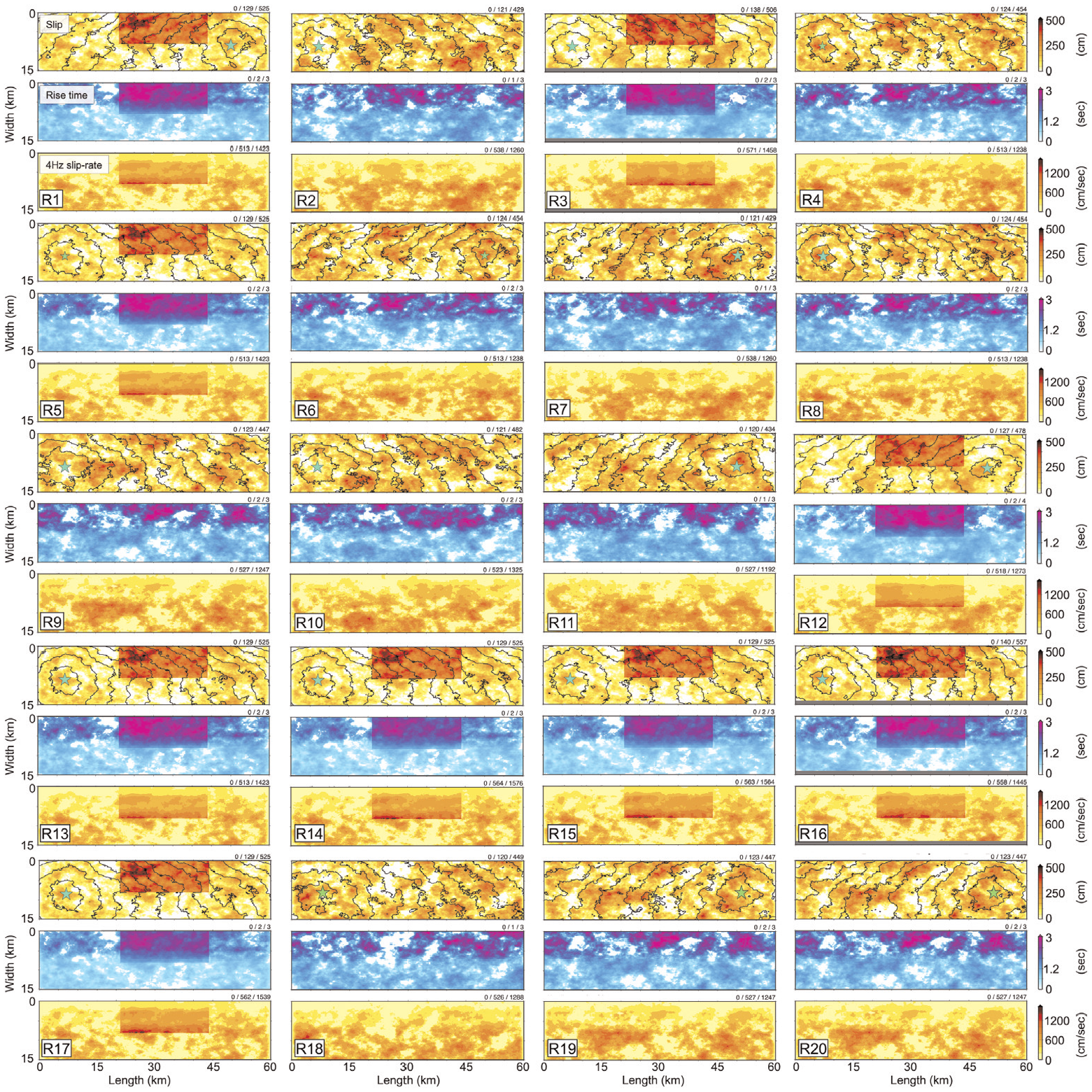
Rupture planes of all realizations: slip distribution (top panel), rise time (middle panel), and4-Hz slip-rate (bottom panel). The black lines represent the rupture front contours at 1 s intervals and the green star the location of the hypocenter.
The top, middle, and bottom panels show the slip distribution, the rise time, and the 4 Hz slip rate, respectively, with the numbers on the top-right corner of each panel indicating the minimum, average, and maximum values of the relevant parameter. The green star denotes the location of the hypocenter on the rupture plane (west view), and the black lines represent the rupture front contours at 1 s intervals (isochrones). A subset of rupture models employs discrete high-slip patches with assigned dimensions and location on the rupture plane, thus originating multiscale slip distributions that incorporate both stochastic small-scale variations of slip (in the background) and deterministically specified areas of high slip. The patches have an area of 23 km × 8 km and are located at the top of the rupture plane and 21 km away from the southern end of the fault (which corresponds to the left edge of the rupture planes in Figure 1). Table 1 provides a summary of the key features of the rupture plane for each realization.
Selected features of the rupture models for each earthquake realization
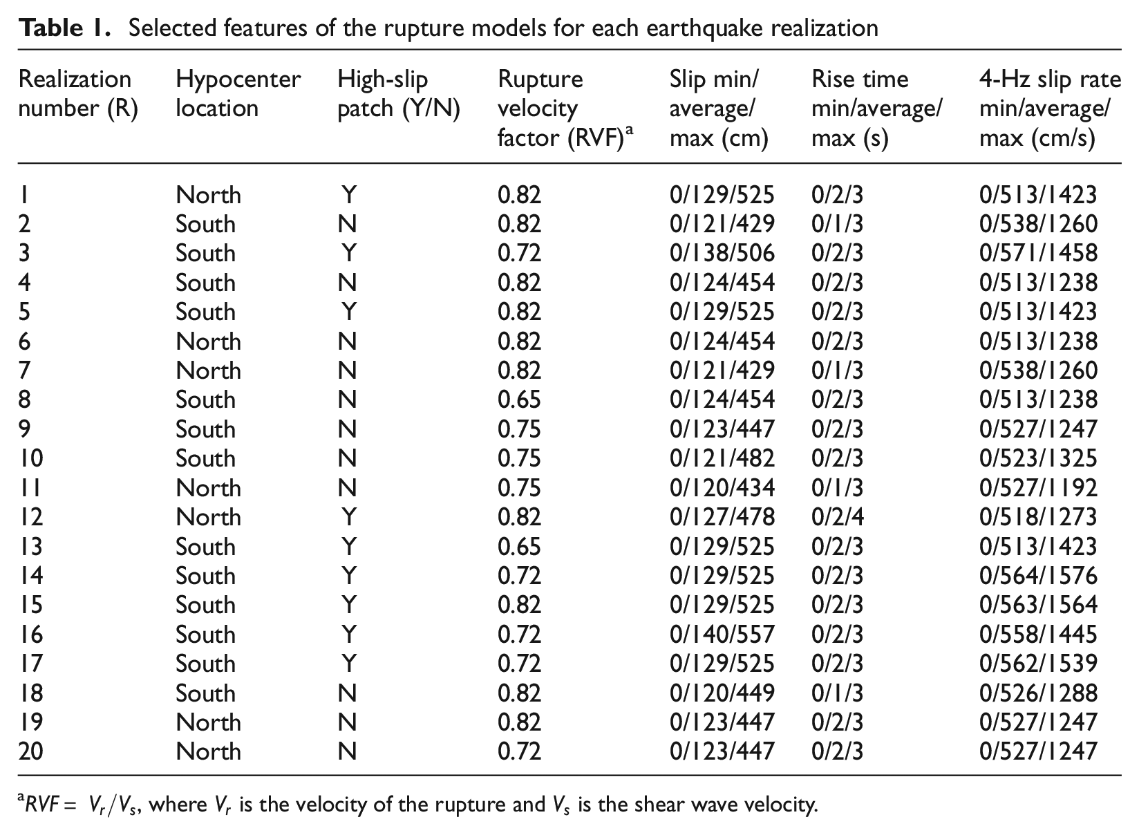
From Figure 1 and Table 1, it is seen that selected pairs of realizations adopt the same rupture parameters and differ only in the location of the hypocenter, which is either at 10 km from the northern tip of the fault (called “north hypocenter”) or at 7 km from the southern tip of the fault (called “south hypocenter”). As such, these realizations are identified as “paired.” See, for example, R2-R7, and R1-R5. In all cases, the rupture initiates at a depth of 8 km on the rupture plane and the rupture top depth (Ztor) is 200 m. While it is not expected that the ground motions resulting from paired realizations will be mirrored because of the heterogeneity of the velocity model and the stochastic nature of the rupture generator, these pairs of simulations are utilized to analyze the effects of forward and backward directivity and interpret the results from the comparisons with the empirical models.
The analyses presented in this study are carried out on the two horizontal components of the ground motions, normal and parallel to the fault, sampled on a 2-km spacing grid, which leads to a total of 2301 × 2 = 4602 ground motions for each realization. In all realizations, the simulations resolve frequencies up to 5 Hz with a minimum shear-wave velocity of 250 m/s. Inelastic attenuation is obtained with frequency-independent P- and S-wave attenuation factors, which relate to the shear wave at the considered grid point.
Figure 2a and b provides a representation of the distribution of the shallow shear-wave velocity (VS30) and the depth to the first occurrence of VS of 1 km/s (Z1.0) across the computational domain (Aagaard and Hirakawa, 2021).
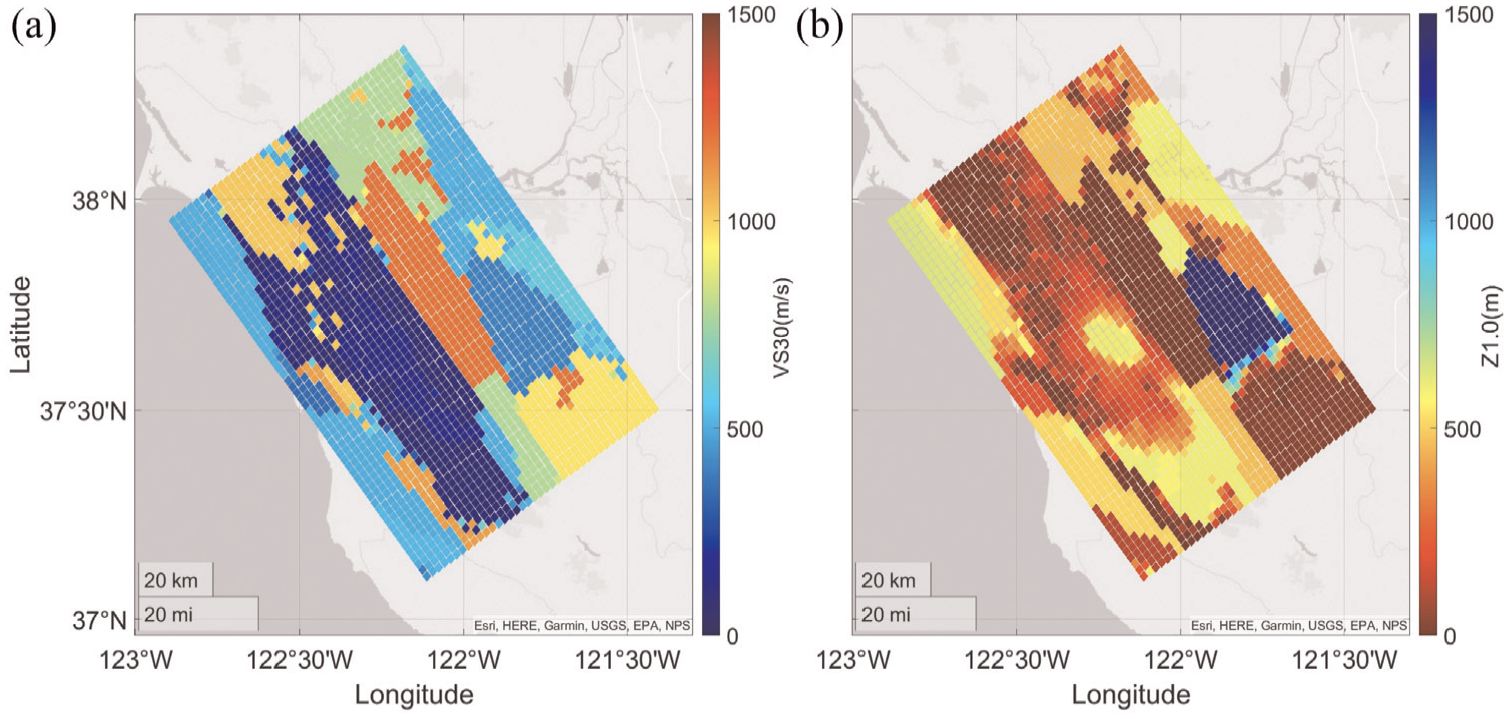
Computational domain: distribution of (a) shallow shear-wave velocity (VS30 in m/s), and (b) depth to the first occurrence of shear-wave velocity of 1 km/s (Z1.0 in m). USGS velocity model (v21.1).
The geology structure in the San Francisco Bay Area is host to a variety of rock and sedimentary units. For example, quaternary surficial sediments with VS30 as low as 81 m/s and Z1.0 ranging between 100 and 600 m characterize the near-fault sites west of the Hayward Fault (dark blue area in Figure 2a); Great Valley rocks with VS30 of about 1200 m/s identify the sites east of the fault (orange area in Figure 2a); and formations of unconsolidated to semi-consolidated beds of gravel, sand, silt, and clay with VS30 of about 400 m/s and Z1.0 of 1400 m distinguish the Pleasanton-Livermore Valley (dark cyan area in Figure 2a). Across the entire computational domain, the median VS30 is 409 m/s, with a standard deviation of 0.94 (in lognormal units), and the median Z1.0 is 0.26 km with a standard deviation of 1.14 (in lognormal units).
Peak ground velocity
The PGV is utilized in this study as an indicator of the forward rupture directivity affecting the motions at sites in the near field and in the direction of rupture propagation. In this study, the definition provided in the ASCE/SEI7 (2022) is utilized as a general reference to distinguish near-field from far-field sites. Figure 3 shows the variation of the simulated PGV (RotD50) as a function of the Joyner-Boore distance, Rjb, across the entire computational domain with overlain GMMs predictions (median ± 1 standard deviation), for each realization (R1 through R20). The color scheme represents the VS30 at each site, consistently with Figure 2a. While comparisons demonstrate a substantial agreement between the simulated peak velocities and the GMMs for all realizations, the simulated PGVs at sites characterized by similar site conditions and distance from the fault (i.e. clusters with the same color) vary substantially across the realizations. A quantitative assessment of such differences is provided in the next section.
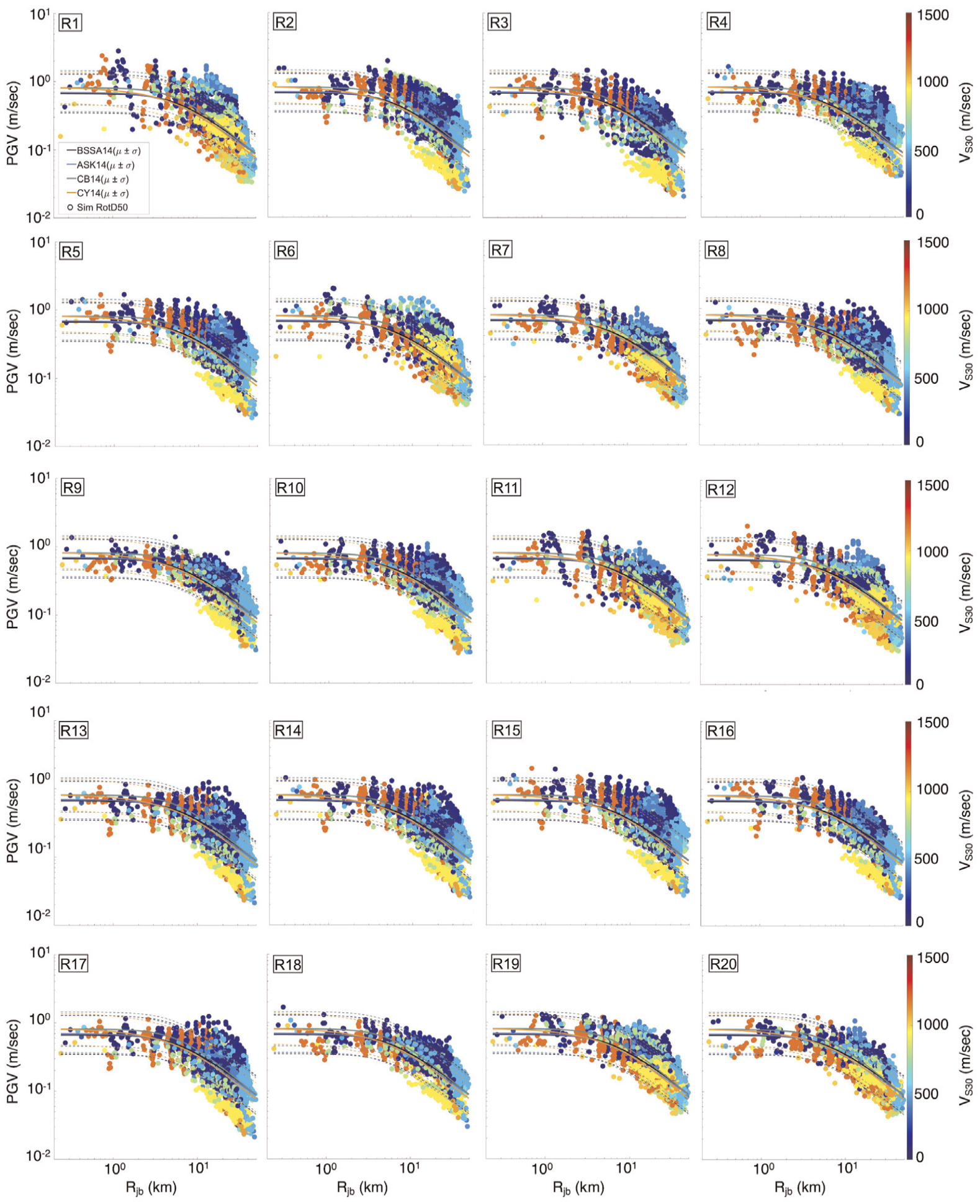
Simulated PGV (m/s) versus Rjb (km) for all realizations (see also Table 1) with overlain NGA-W2 GMMs’ predictions. The color code represents the VS30.
Convolving the information in Figures 1 and 3 demonstrates that the highest values of the PGV manifest when the corresponding clusters of sites are located in the forward-directivity direction, with peaks attained when the rupture model features high-slip patches in the rupture direction. This is seen to have implications on the PGV absolute values up to 30 km from the fault, as it will be discussed later, as well as on PGV variability across sites equidistant from the fault. Table 2 provides a summary of the PGV standard deviation (in lognormal units) at selected distances (bins) from the fault showing differences in the spread by factors above 2. See, for example, R3 and R9 at 5 km from the fault, and R2 and R20 at 30 km from the fault. For each sampled distance, the minimum values of the standard deviation are underlined, and the maximum values are underlined and bold.
Standard deviation of the PGV in lognormal units at selected distances from the fault
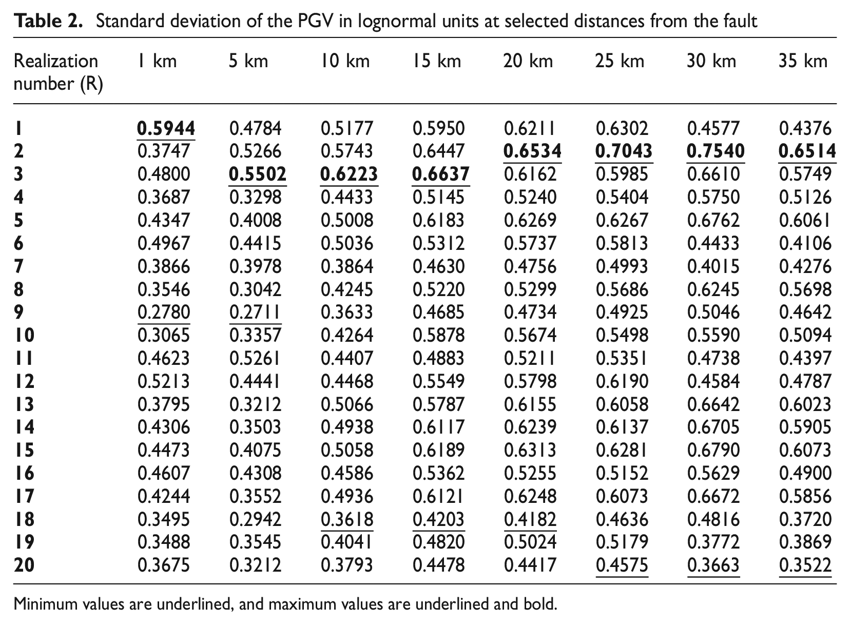
Minimum values are underlined, and maximum values are underlined and bold.
From the structural risk evaluation perspective, this indicates that rupture models differing for the slip distribution and rate, while having the same dimensions and hypocenter location, can lead to substantially different distributions of the ground-motion peak amplitudes at sites equidistant from the fault, with implications on the expected infrastructure response variability.
Averaged over all the realizations with different propagation directions, the total standard deviation of the PGV is on the order of 0.41–0.64 (in lognormal units), which is aligned with the standard deviations predicted by the NGA-W2 GMMs, ranging from 0.53 to 0.65 across the different models.
Figure 4 shows the variation of the PGV with the distance for all combined realizations (2301 × 20 = 46,020 gray dots) with corresponding median and standard deviation at sites equidistant from the fault (red dots and lines) and overlain NGA-W2 GMMs (median ± 1 standard deviation).
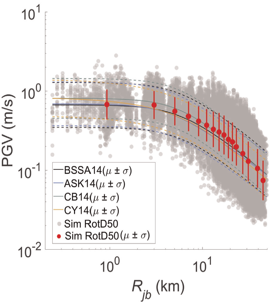
PGV vs Rjb: Median (μ) and standard deviation (σ) of the simulated PGV calculated across the 20 realizations and corresponding NGA-W2 GMMs.
Analysis approach
Following the evidence from Figure 3 and given the pronounced geological heterogeneity of the region, two approaches were employed to compare simulated ground motions and empirical models. The first one considers the median properties of the entire regional domain to calculate the GMMs’ predictions; the second one partitions the regional domain into subdomains characterized by approximately homogeneous VS30. The criteria set forth in the ASCE/SEI7 (2022) to define site classes are utilized to identify such clusters of sites (i.e. subdomains).
Specifically, the entire region is divided into five clusters: subdomain 1 with a variety of very loose, loose, and medium dense sand or soft, medium stiff, stiff clay (classes F to D); subdomain 2 with dense sand or very stiff clay (class CD); subdomain 3 with dense sand or hard clay (class C); subdomain 4 with soft rock (class BC); and subdomain 5 with medium hard rock (class B). Figure 5a offers a representation of the computational domain with the partition into subdomains, each of which is represented with a different color. Figure 5b summarizes the statistics (median and standard deviation in lognormal units) of VS30, Z1.0, and Z2.5 for the full domain and for each subdomain, providing a measure of the consistency of VS30 within each subdomain. The dispersion of Z1.0 (sigma) within each subdomain is seen to decrease compared with the full domain, demonstrating an improved homogeneity of Z1.0 within each subdomain as well.
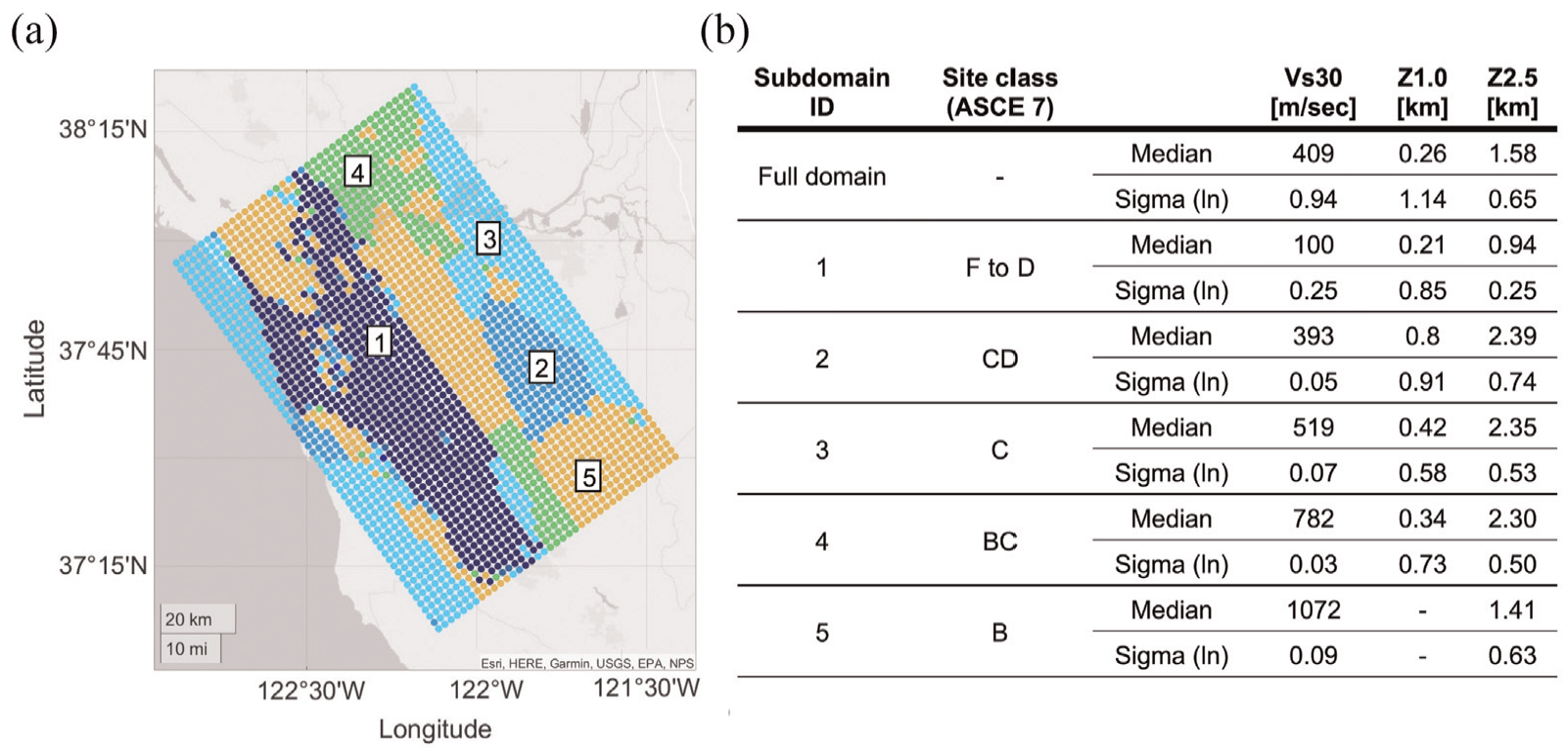
(a) Partition of the computational domain into subdomains (1 through 5) based on the site classes definition in ASCE/SEI 7; (b) median and standard deviation (in lognormal units) of VS30, Z1.0, and Z2.5 for the full domain and for each subdomain.
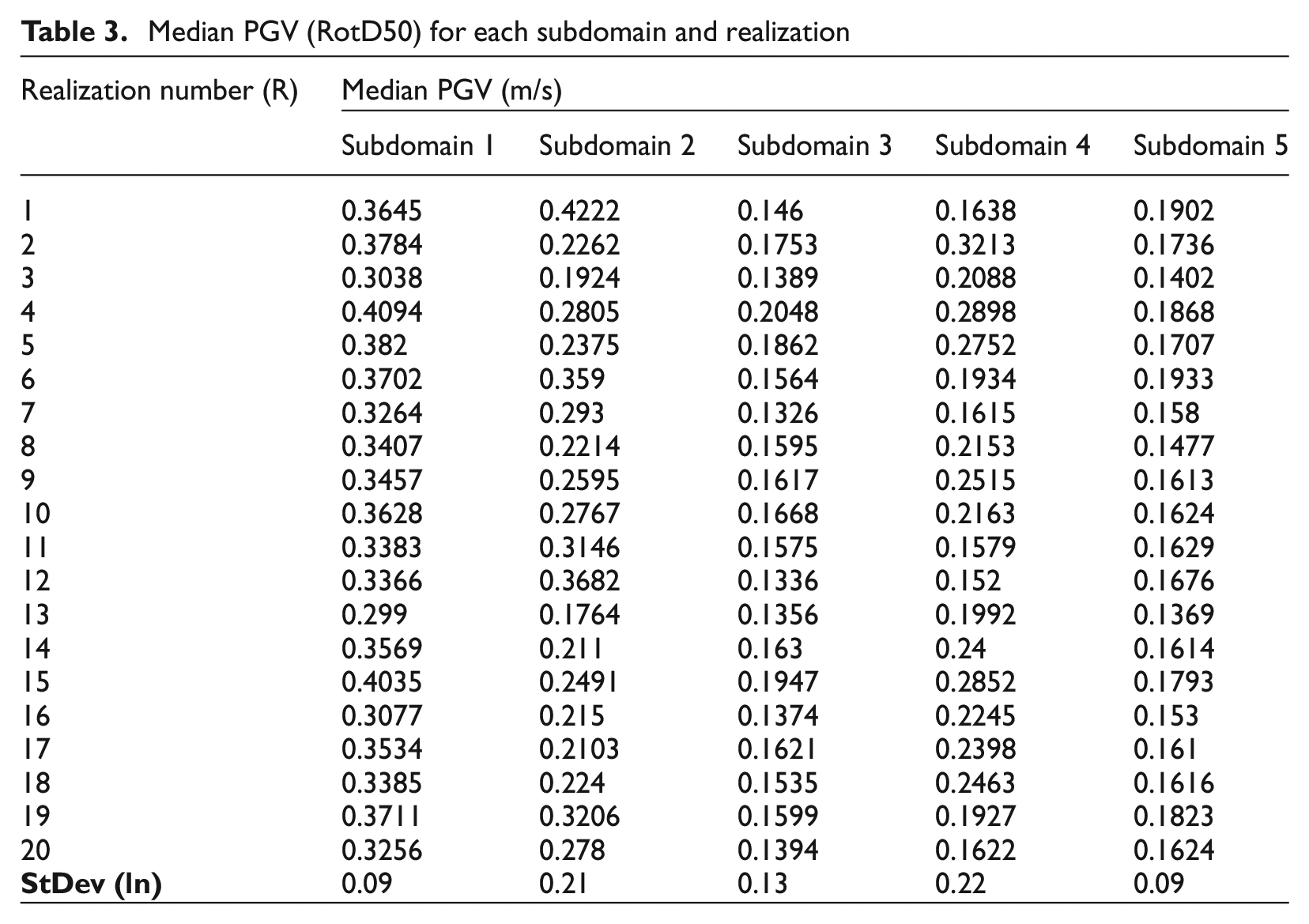
The partition of the domain into subdomains is first utilized to assess the variability of the median simulated PGV across all realizations and for each subdomain. These data are summarized in Table 3, demonstrating variations in the medians up to a factor of 2.4 for subdomain 2 with the largest spread observed in subdomains 2 and 4. As discussed later, these are the subdomains with ground-motion amplitudes most sensitive to the effects of rupture directivity due to their spatial location with respect to the fault and to site conditions.
Median PGV (RotD50) for each subdomain and realization
The analyses of the type presented in Figure 3 were performed subdomain by subdomain with the intent to isolate the effects of site conditions and rupture directivity. For the sake of conciseness, only the results of R2 and R7 are discussed in detail, but the same considerations remain valid across all realizations. R2 and R7 are paired and adopt a rupture model characterized by an average slip of 121 cm and a maximum slip of 429 cm. In R2, the rupture initiates close to the southern tip of the fault, while in R7 it initiates close to the northern tip.
Figure 6 shows the variation of the simulated PGV with the distance for R2 across the entire domain and for each subdomain, with overlain PGV predicted by the NGA-W2 GMMs. The median parameters specific to the full domain and each subdomain (i.e. VS30, Z1.0, Z2.5) are utilized as an input for the GMMs. The dots represent the simulated PGV at each station and are colored in gray if they are within the median ± 1 standard deviation envelope of the empirical models, in cyan if they fall above the envelope, and in pink if they fall below the envelope. Finally, the black dots represent the median simulated PGVs at sites equidistant from the fault (2-km bins).
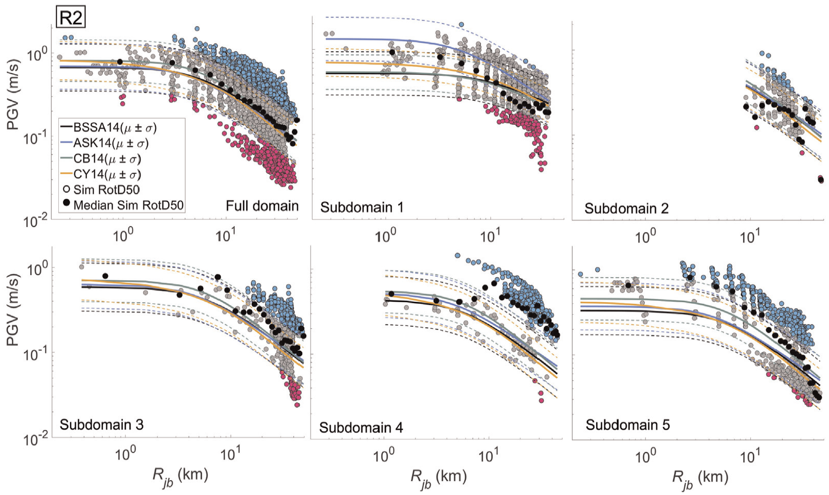
Realization 2: PGV vs distance from four NGA-W2 GMMs (median ± 1 standard deviation) and simulations for the full domain and for each subdomain. The colors gray, cyan, and pink indicate that the simulated PGVs are within, above, and below the empirical models’ envelope, respectively. The black dots represent the median of PGVs at sites equidistant from the fault.
It should be noted that the median site conditions for subdomain 1 are outside the range of applicability of the NGA-W2 GMMs (median VS30 = 100 m/s), and that the simulations resolve a minimum shear-wave velocity of 250 m/s, thus introducing approximations in the prediction of the ground-motion intensities. However, comparisons are still reported and utilized as a general reference to inform the interpretation of the simulation results.
The analysis conducted across the full domain shows that the median simulated PGVs vary with Rjb closely to the median empirical models’ predictions, with two distinct populations of sites with PGV above and below the GMMs envelopes. Such sites are identified with the same color code in the maps of Figure 7 (top-left, full domain), roughly indicating that the sites with PGVs above the GMMs envelope are in the direction of the rupture propagation, while those below the GMMs envelope are in the backward direction.
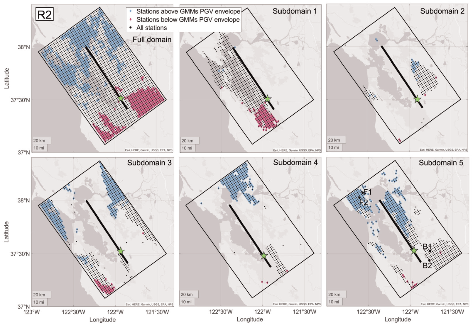
Realization 2. Maps representing the spatial distribution of the stations in the computational domain. The black dots indicate the stations belonging to each subdomain (or full domain). Cyan and pink are utilized to identify the stations for which the simulated PGVs are above or below the GMMs’ envelope, respectively. The black line represents the projection of the segment of the Hayward fault modeled in this study. The green star indicates the location of the hypocenter (south).
However, the plots and maps generated for each subdomain (Figures 6 and 7) clearly demonstrate that the stations with simulated PGVs above and below the NGA-W2 GMMs envelopes are consistently sited in the forward and backward directivity, respectively, with selected subdomains yielding median PGVs (black dots) above the GMMs envelope. The soft rock sites of subdomain 4 in the northern region of the computational domain provide one of such examples. Noteworthy, these sites are all located about 70 km away from the epicenter and in the vicinity of the tip of the fault, where the constructive interference of the S-waves caused by the propagation of the rupture is expected to manifest the strongest effects (Somerville et al., 1997). A similar trend is observed for medium/hard rock near-field sites in subdomain 5, where the PGVs at locations within 10 km from the fault are on the upper bound of the GMMs envelope.
Considering this evidence, the subdomains in the near field with ground-motion intensities potentially influenced by forward-directivity effects are compared with the model proposed by Bray and Rodriguez-Marek (2004), BR-M04 hereafter. The BR-M04 relationship was developed with ground motions from shallow crustal earthquakes identified as forward directivity based on the geometric conditions delineated in Somerville et al. (1997). The ground motions utilized to derive the model were recorded at sites less than 20 km from the causative fault, from events with moment magnitudes ranging from 6 to 7.6. Results of this comparison are shown in Figure 8 (top row) for subdomains 2, 4, and 5 up to 20 km, demonstrating a substantially improved agreement between the fault-normal component of the simulated PGVs and the prediction of the empirical model, with the median PGVs laying within median ± 1 standard deviation of the BR-M04 model.
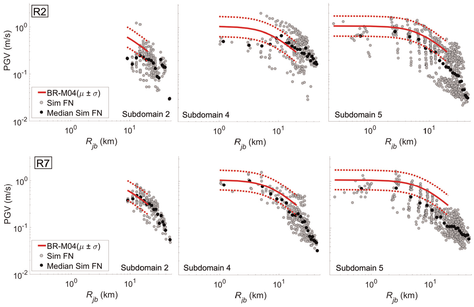
Simulated fault-normal PGV (m/s) vs Rjb (km) for subdomains 2, 4, and 5 and realizations R2 and R7 with overlain BR-M04 model’s prediction for forward-directivity ground motions in the near field (0–20 km as per BR-M04).
This evidence is utilized to assess the realistic character of the simulated PGVs at sites located along the strike where directivity pulses due to the forced unilateral rupture propagation control ground-motion amplitudes. Further comparisons between the simulated motions and a subset of the recordings utilized by BR-M04 are presented in the next sections in terms of PGV, waveforms, and structural response.
It should also be noted that the maximum PGVs (fault normal) in Figure 8 attain values of about 2 m/s at 5 km from the fault. Similar values have been observed in historical earthquakes. Examples include the M6.69 1994 Northridge earthquake with a fault-normal PGV of 1.73 m/s at the Rinaldi receiving station with a closest distance to the fault plane of 7.1 km.
The analyses carried out for R2 are repeated for R7, where the rupture initiates close to the northern end of the fault. The results are summarized in Figures 9 and 10. The observations related to R2 can be extended to R7, noting that the sites with PGV above the GMMs envelope are mainly located where the rupture propagates unilaterally along the strike (toward south), while those with PGV below the envelope are in the backward directivity direction (toward north). Similar to the observations for R2, the comparison with the BR-M04 model in Figure 8 (bottom row) supports the evidence that the high PGVs are associated with forward-directivity effects at sites in the vicinity of the fault tip in subdomain 4 and in the near field along the strike in subdomain 5.
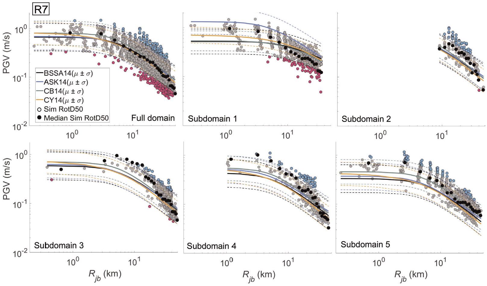
Realization 7: PGV vs distance from four NGA-W2 GMMs (median ± 1 standard deviation) and simulations for the full domain and for each subdomain. The colors gray, cyan, and pink indicate that the simulated PGVs are within, above, and below the empirical models’ envelope, respectively. The black dots represent the median of PGVs at sites equidistant from the fault.
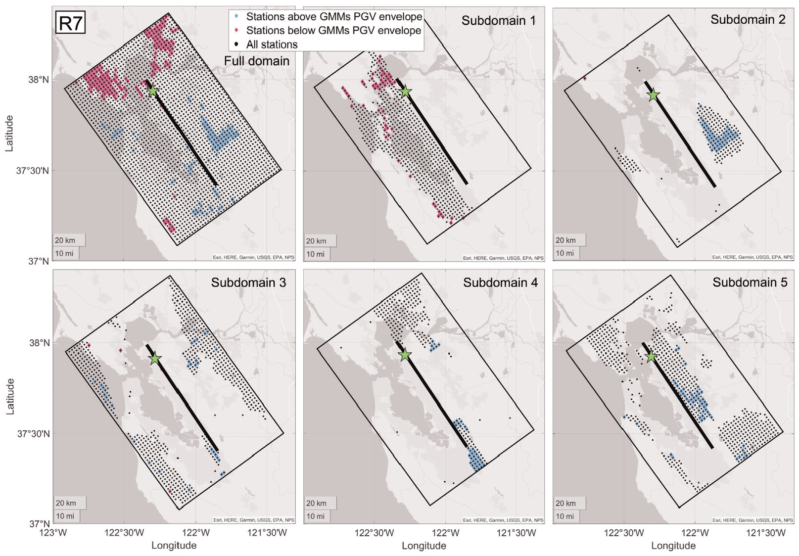
Realization 7. Maps representing the spatial distribution of the stations in the computational domain. The black dots indicate the stations belonging to each subdomain (or full domain). Cyan and pink are utilized to identify the stations for which the simulated PGVs are above or below the GMMs’ envelope, respectively. The black line represents the projection of the segment of the Hayward fault modeled in this study. The green star indicates the location of the hypocenter (north).
Noteworthy, amplifications of the motions are also seen in the Pleasanton-Livermore Valley (subdomain 2) at distances up to 30 km from the fault. This region is characterized by a median VS30 of 390 m/s and a median Z1.0 of 1.4 km. In these conditions, ground-motion amplitudes can be partially influenced by the effect of constructive interference of the S-waves in the rupture propagation direction and, to a larger extent, by the buildup of waves trapped in this softer soil basin. Such amplifications have been observed in sedimentary basins in moderate and large earthquakes, including the 1985 Michoacan, Mexico (Anderson et al., 1986), the 1994 Northridge (Gao et al., 1996) and the 1999 Chi-Chi (Fletcher and Wen, 2005), emphasizing how localized basin structures may result in larger motion amplitudes than predicted by the empirical models.
Based on this evidence, it was decided to examine realizations in which the combined effect of forward directivity, localized rupture high slips, and local site conditions may lead to strong, yet realistic, motions that current empirical models do not represent. R1 and subdomain 2 provide one such example. The rupture model in R1 is characterized by north hypocenter and a patch with a maximum slip of 525 cm. Subdomain 2 (Pleasanton-Livermore Valley) hosts unconsolidated to semi-consolidated granular deposits embedded in a stiffer soil structure.
Figure 11a shows how the simulated PGVs (RotD50) compare with the NGA-W2 GMMs, demonstrating that the peak velocities are outside the GMMs’ envelope for 76% of the stations, with the median PGVs at sites equidistant from the fault laying above the envelope up to 30 km from the rupture plane. The spatial distribution of these stations is represented in Figure 11c with cyan color. The comparison of the fault-normal PGV with the BR-M04 model in Figure 11b shows that 64% of the stations within 20 km have PGVs above median ± 1 standard deviation with medians right on the upper bound of the BR-M04 84th percentile, pointing to additional factors potentially contributing to the strength of the motions. The high amplitudes also manifest in the PSAs, with amplitudes reaching the upper bound of the NGA-W2 GMMs envelope in the 1- to 10-s bandwidth (Figure 11d). Mapping the rupture plane on the computational domain demonstrates that the Pleasanton-Livermore Valley is in the forward rupture direction and in the proximity of the high-slip region (red rectangle along the fault in Figure 11c), which has been associated with a significant increase of the motion amplitudes (Eckert et al., 2022; Pitarka et al., 2019). Figure 11e and f reports the velocity time histories for the two separate components (fault normal and fault parallel) of two sites, namely, site A, which is on medium/hard rock, and site B, which is on semi-consolidated incoherent soil. The two sites are about 10 km apart. The motions are seen to have larger amplitude and longer duration at site B than at site A, which is caused by the reflection of waves occurring in the Pleasanton-Livermore Valley. Noteworthy, the fault-parallel component of station B shows a two-sided pulse with amplitudes larger than in the fault-normal component, which results from local basin amplification effects that modify the original features of the ground-motion components.
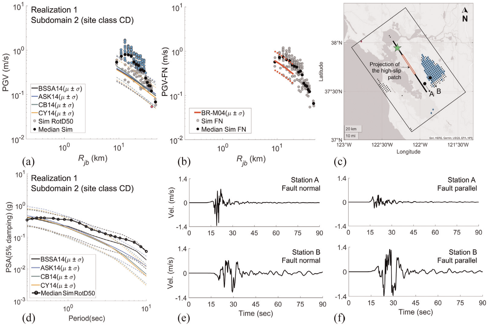
Realization 1, subdomain 2: (a) simulated PGV (RotD50) vs Rjb with overlain NGA-W2; (b) simulated PGV (fault normal) vs Rjb with overlain BR-M04 GMM; (c) map of subdomain 2 with cyan and pink colors indicating the sites with simulated PGV above and below the NGA-W2 GMMs envelope respectively; (d) PSA vs spectral periods with overlain NGA-W2 GMMs; and (e–f) velocity time histories at stations A and B.
Therefore, although standing as “outliers” when compared with the empirical models, these simulated ground motions result from the concurrent effects of directivity, rupture characteristics, and local site conditions that collectively lead to the amplification of the seismic motions expected from the underlying physics of the simulated earthquake phenomenon. The identification of these conditions is crucial to interpreting simulation results and informing the selection of simulation parameters yielding ground-motion amplitudes not adequately represented in the catalog of observational ground-motion data.
To further investigate the characteristics of the motions with simulated PGV outside the NGA-W2 GMMs envelope, selected time histories are analyzed and compared with historical records. Figure 12a and c shows the velocity time histories of the simulated motions (fault normal) at two sites located in the forward-directivity direction, while Figure 12b and d reports the simulated velocity time histories (fault normal) at two sites located in the backward directivity direction. The motions are both from R2 subdomain 5 and are identified with “F1” and “F2” (where F stands for forward) and “B1” and “B2” (where B stands for backward) in Figure 7. Figure 12e and f shows the velocity time histories (fault normal) of the 1992 Landers Earthquake at the Lucerne station, which is located 45 km from the epicenter and 1.1 km away from the fault (forward direction), and at the Joshua Tree station, which is near the epicenter (backward direction) (Somerville et al., 1997). Strong similarities are seen in the simulated and real motions, with the sites in the rupture forward directivity exhibiting a large, short-duration pulse occurring at the beginning of the motion, and the sites in the rupture backward directivity showing low amplitudes.
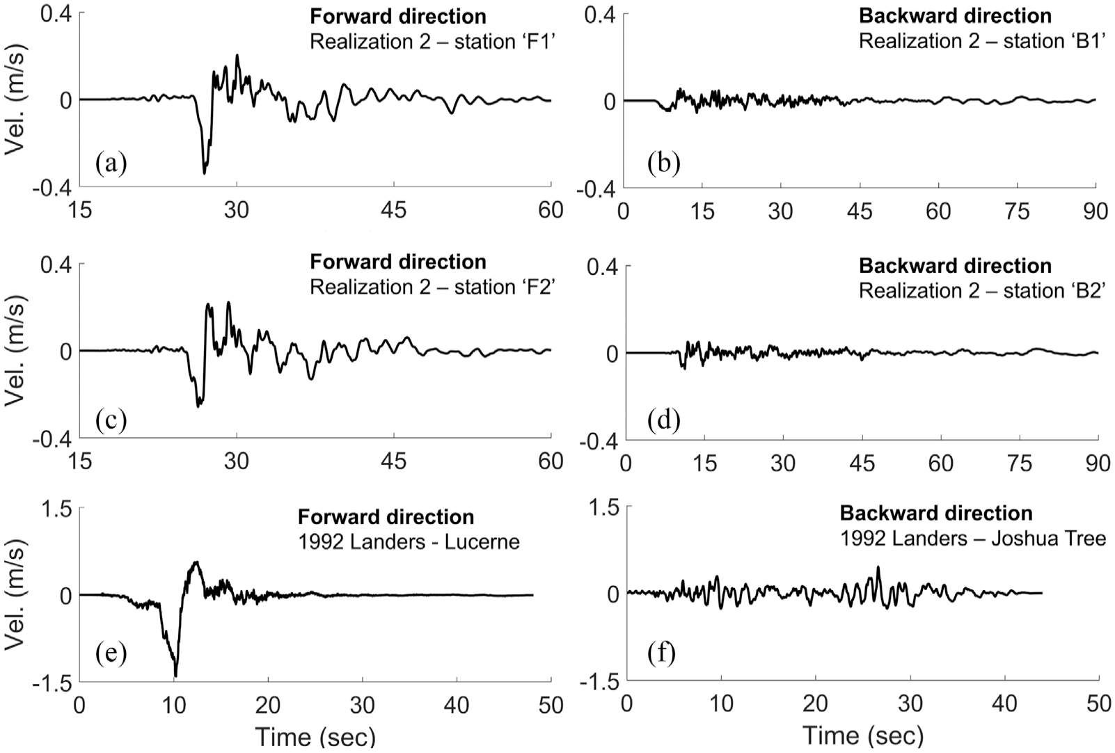
Velocity time histories for three sites in the forward-directivity direction (a–c) Realization 2, station “F1” and “F2” in subdomain 5, (e) 1992 Landers earthquake, Lucerne station, and three sites in the backward directivity direction (b–d) Realization 2, station “B1” and “B2” in subdomain 5, and (f) 1992 Landers earthquake, Joshua Tree station.
The observations made here for selected realizations and sites can be extended to all realizations, demonstrating that PGVs falling above the predictions of the empirical models possess the key features of motions generated under similar tectonic conditions in real earthquakes. Figures S1 and S2 in the supplemental material show how the PGV and PSA compare with the GMMs across all realizations, for the full domain.
Determining the reliability of simulated motions from large-magnitude events as a function of the specificity of the modeled region (i.e. seismic velocity structure) and the adopted rupture model has important implications for hazard and risk assessments. Considering these results, simulation data of this type can in fact be used to inform the update of current GMMs and hazard estimates and broaden empirical data for ground-motion selection to perform seismic evaluations of structural systems. Early examples of how ground-motion simulations can be utilized in code-compliant designs can be found in Matinrad and Petrone (2023) and Taslimi and Petrone (2024).
In the next section, selected populations of motions exhibiting extreme PGVs are analyzed and compared with earthquake records in terms of demand posed to a building structure.
Implications for structural response
A 20-story steel moment-resisting frame building model (Wu et al., 2018) is utilized to assess the response of a realistic structure subject to simulated and recorded motions exhibiting forward-directivity characteristics. The selection of a high-rise building is primarily motivated by the sensitivity of tall structures to long-period velocity pulses that characterize forward-directivity ground motions. In addition, as detailed below, the periods of the fundamental and higher modes of vibration of the considered structure are fully resolved by the considered ground-motion simulations (max frequency is 5 Hz), which is crucial to ensure reliability of the obtained structural response.
The building is modeled as a planar structure with the OpenSees software, employing force-based elements with multiple integration points and fiber cross-sections to simulate material and geometrical nonlinearities. The building’s fundamental periods are T1 = 2.68 s, T2 = 0.93 s, and T3 = 0.54 s.
The simulated motions from R1 (subdomains 2 & 5) and R2 (subdomain 4), and a subset of the population of records utilized by Bray and Rodriguez-Marek (2004) and resolved in the fault-normal and fault-parallel components by Baker et al. (2011) are utilized. Table 4 lists the considered earthquakes and stations, as well as selected key features, including moment magnitude (M), faulting mechanism, closest distance from the fault (R), PGV of the fault-normal component (PGV-FN), and PGV of the fault-parallel component (PGV-FP).
List of earthquakes, stations, and key parameters
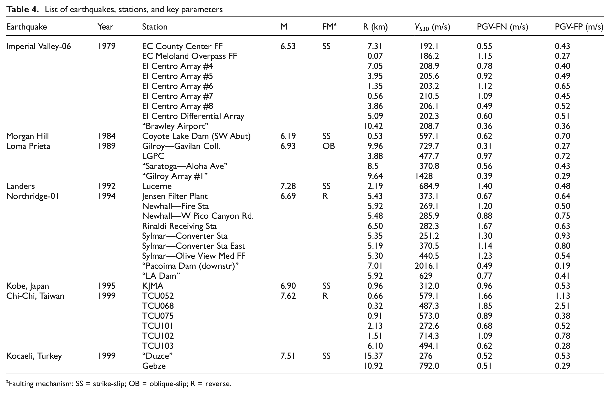
Faulting mechanism: SS = strike-slip; OB = oblique-slip; R = reverse.
Although the sites exhibiting forward directivity are known to be distributed near the fault at different distances from the epicenter depending on the faulting mechanism, the key characteristics of the motions remain unvaried. The radiation pattern of the shear dislocation on the fault, in fact, causes a large pulse of motion oriented in a direction perpendicular to the fault plane (Somerville et al., 1997). Therefore, the analyses presented in this section aggregate earthquake events with different faulting mechanisms (strike-slip, oblique, and reverse), and focus on the FN component of the motions without consideration of their spatial distribution with respect to the epicenter.
Figure 13 shows the variation of the PGV-FN as a function of the distance from the fault for the three selected sets of simulated motions (R1, subdomains 2 & 5 and R2, subdomain 4) and the records in Table 4, indicating analogous trends across a range of distances.
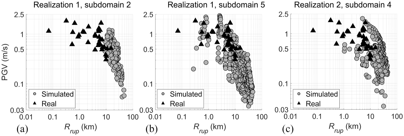
Variation of the PGV-FN with distance (Rrup). Simulated ground motions from (a) Realization 1 subdomain 2, (b) Realization 1 subdomain 5, and (c) Realization 2 subdomain 4 vs the ground-motion records in Table 4.
These populations of motions up to 20 km are utilized to perform nonlinear time-history analyses with the 20-story building. The peak interstory drift ratio (PIDR) is utilized as the key engineering demand parameter to estimate damage to structural components. The ASCE 7-22 (ASCE/SEI7, 2022), the Eurocode EN 1998-1 (European Committee for Standardization (CEN) 2004), and the New Zealand Standard NZS 1170.5 (SNZ 2004) are just some examples of the utilization of maximum allowable drifts in the design to assess structural demands and control damage. The plots in Figure 14 compare the variation of the PIDR as a function of the PGV-FN for the sets of simulated and recorded motions only for sites within 20 km, demonstrating a strong similarity in the trend of data for building responses ranging from substantially linear (PIDR < 1%) to highly nonlinear (PIDR > 2.5%). In the context of assessing the realistic character of the simulated motions, particularly when selected IMs lay outside the range predicted by the empirical models, analyses of this type indicate that the simulations utilized in this study have the key features of consistent records and yield the expected response for a realistic structure.
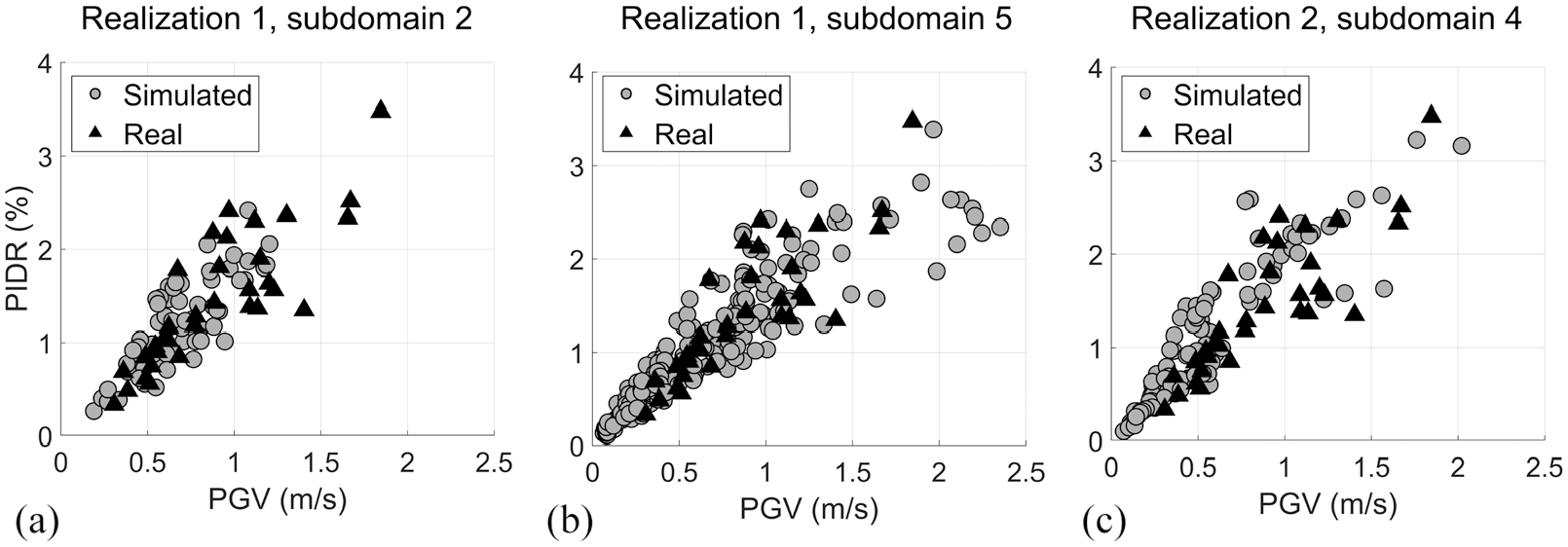
Twenty-story building: PIDR vs PGV-FN. Simulated ground motions from (a) Realization 1 subdomain 2, (b) Realization 1 subdomain 5, and (c) Realization 2 subdomain 4 vs the ground-motion records in Table 4.
The populations of motions in Figures 13 and 14 cover site class CD (very dense sand and stiff clay), where forward directivity is accompanied by local wave amplifications, and near-field site class BC (soft rock) and class B (medium hard rock), overall spanning distances from 1 to 50 km. As such, these motions can be reliably utilized to supplement the population of measured ground-motion records when interested in structural assessments under strong excitations. This is expected to enable more realistic evaluations of the structural response variability for assigned values of the IMs (PGV in this case), which is currently hindered by the utilization of a limited number of motions.
Concluding remarks and ongoing work
This study analyzes a set of simulated ground motions generated from 20 M7 Hayward fault strike-slip scenario earthquakes in the San Francisco Bay Area. The analyses presented in this article provided the basis to inform the selection and assessment of the simulation scenarios to share on a publicly available platform under a joint effort of the Lawrence Berkeley National Laboratory and the PEER Center.
The primary objective of this work was to evaluate the realistic character of the simulated motions as a function of the features of the employed rupture model (Graves and Pitarka, 2016; Pitarka et al., 2019) and seismic velocity structure (Aagaard and Hirakawa, 2021). Specific focus was paid to simulation parameters yielding ground-motion PGVs outside the predictions of state-of-the-art ergodic empirical models. Specifically, four NGA-W2 GMMs (Abrahamson et al., 2014; Boore et al., 2014; Campbell and Bozorgnia, 2014; Chiou and Youngs, 2014) and the model proposed by Bray and Rodriguez-Marek (2004) for forward-directivity motions in the near-field were utilized.
The analyses carried out on the aggregated motions from the full domain demonstrated that differences in the rupture model parameters (stochastic small-scale rupture variability and incorporation of high-slip patches) can produce differences in the prediction of peak velocities up to 2.4 times for clusters of sites characterized by similar shallow shear-wave velocity and depth to the first occurrence of VS = 1 km/s. In addition, differences of the order of 2× are observed in the variability of the PGV at sites equidistant from the fault as a function of the rupture parameters, and regardless of the site conditions.
Based on this evidence and considering the heterogeneity of the seismic velocity structure of the region, an approach based on the identification of subdomains having consistent shallow shear-wave velocity (VS30) was adopted. The criteria set forth in the ASCE/SEI7 (2022) to define site classes were employed to partition the domain into five subdomains. The PGVs falling outside (above and below) the NGA-W2 GMMs envelopes for the separate subdomains were consistently identified as spatially located in the forward and backward rupture directivity across all realizations and site classes. This was confirmed by a further comparison performed with the BR-M04 model, showing a strong agreement between the simulated and predicted PGVs in the forward-directivity.
High values of the PGV were also observed in earthquake realizations where the combined effect of high-slip patches located in the rupture forward direction and local site conditions contributed to generating strong motions. In the analyzed region, this was the case for the Pleasanton-Livermore Valley, in which motions at sites up to 20 km far from the fault manifest peaks in the fault-normal ground velocities above the median + 1 standard deviation predicted by the BR-M04 model. In this area, the median values of the PGVs at sites equidistant from the fault are seen to lay right on the median + 1 standard deviation boundary.
Sites in the rupture forward and backward directions were also compared with selected records from the 1992 Landers earthquake. The simulated velocity time histories of the fault-normal component confirmed that the simulations retain the characteristics of the records from similar tectonic conditions, including large-amplitude pulses occurring at the beginning of the time history in the forward-directivity sites and small-amplitude motions in the backward directivity sites.
Furthermore, the fault-normal component of a subset of records identified as near-fault forward-directivity by Somerville et al. (1997) was utilized to assess the response of a 20-story moment-resisting steel frame building and compare it with that obtained from the fault-normal component of selected sets of simulated motions (from two realizations and three subdomains). Both the variation of the PGV as a function of the distance from the fault and the variation of the PIDR as a function of the PGV showed strong similarities between the sets of motions.
Overall, the analyses carried out in this study demonstrated that strong ground motions at distances up to 30 km from the fault can be obtained in physics-based simulations when the following factors act concurrently: (1) the sites are located in the rupture forward directivity, (2) the rupture model incorporates high-slip patches in the forward-directivity direction, and (3) the site resides where the local geological conditions can produce ground-motion amplification.
Findings from this work provide a path for interpreting ground-motion site and event specificity obtained from a suite of physics-based simulation models to inform the selection of simulation scenarios for site-specific engineering analyses under strong motions.
Finally, comparing PGV predictions calculated using the NGA-W2 GMMs to those generated from the physics-based scenarios points to the possibility that existing regional hazard models may underestimate ground-motion intensities in selected regions in the San Francisco Bay Area, highlighting the importance of correctly estimating the concurrent effects of rupture directivity and local basin amplification. This information is key to improving our understanding of regional risk.
In light of the results discussed in this article, ongoing work is focused on the identification of rupture models that can provide a realistic representation of the expected ground-motion variability, including the incorporation of simulation parameters leading to strong motions in the San Francisco Bay Area at near and far-field sites and the consideration of a balanced set of unilateral and bilateral ruptures.
Supplemental Material
sj-tiff-1-eqs-10.1177_87552930241265132 – Supplemental material for Ground-motions site and event specificity: Insights from assessing a suite of simulated ground motions in the San Francisco Bay Area
Supplemental material, sj-tiff-1-eqs-10.1177_87552930241265132 for Ground-motions site and event specificity: Insights from assessing a suite of simulated ground motions in the San Francisco Bay Area by Floriana Petrone, Arsam Taslimi, Majid Mohammadi Nia, David McCallen and Arben Pitarka in Earthquake Spectra
Supplemental Material
sj-tiff-2-eqs-10.1177_87552930241265132 – Supplemental material for Ground-motions site and event specificity: Insights from assessing a suite of simulated ground motions in the San Francisco Bay Area
Supplemental material, sj-tiff-2-eqs-10.1177_87552930241265132 for Ground-motions site and event specificity: Insights from assessing a suite of simulated ground motions in the San Francisco Bay Area by Floriana Petrone, Arsam Taslimi, Majid Mohammadi Nia, David McCallen and Arben Pitarka in Earthquake Spectra
Footnotes
Acknowledgements
The authors would like to thank Dr. Sean Ahdi for providing valuable comments that helped improve the quality of the paper. The development of the simulated ground motions utilized in this study was supported by the U.S. Department of Energy Office of Cyber Security, Energy Security and Emergency Response at Lawrence Berkeley National Laboratory. The simulation data in this research used resources of the Oak Ridge Leadership Computing Facility, which is a DOE Office of Science User Facility supported under Contract DE-AC05-00OR22725.
Declaration of conflicting interests
The author(s) declared no potential conflicts of interest with respect to the research, authorship, and/or publication of this article.
Funding
The author(s) disclosed receipt of the following financial support for the research, authorship, and/or publication of this article: The work presented in this study was supported by the Transportation System Research Program of the Pacific Earthquake Engineering Research Center (PEER), through the Award AWD-01-00003574 at the University of Nevada Reno. Any opinions, findings, and conclusions or recommendations expressed in this material are those of the authors and do not necessarily reflect those of the funding agency. Arben Pitarka’s work was performed at the Lawrence Livermore National Laboratory under Contract DE-AC52-07NA27344.
Research Data and Code Availability
The unprocessed ground-motion data will be available in a new expanded simulated ground-motion database under development with PEER.
Supplemental material
Supplemental material for this article is available online.
References
Supplementary Material
Please find the following supplemental material available below.
For Open Access articles published under a Creative Commons License, all supplemental material carries the same license as the article it is associated with.
For non-Open Access articles published, all supplemental material carries a non-exclusive license, and permission requests for re-use of supplemental material or any part of supplemental material shall be sent directly to the copyright owner as specified in the copyright notice associated with the article.