
Abstract
Stochastic ground motion simulation models are often less accurate at lower frequencies than at higher frequencies when fitting recorded data unless supplemented by a deterministic forward directivity velocity pulse model. Moreover, time-modulated stochastic models, which adjust ground motion amplitudes over time, typically use functions that fail to capture multiple strong-motion phases. The February 2023 Turkey (Türkiye) earthquake exhibited diverse recordings, including near-fault and far-field motions with pulse-like and non-pulse-like characteristics, along with single and multiple strong-motion phases. To better represent such a diverse set of recordings, this study enhances a fully non-stationary site-based stochastic model without combining it with a deterministic model. Improvements include a new band-pass filter with upper- and lower-frequency limits, which refines the representation of the low-frequency content. Moreover, a time-modulating function that can represent energy arrival in multiple strong phases is introduced. The reference model’s parameters are identified by fitting to the energy content, zero-level crossings, and cumulative counts of positive-minima and negative-maxima of a target accelerogram. This fitting procedure is modified to address the increased number of parameters. These improvements broaden the reference model’s applicability while preserving its simplicity, a key aspect appealing to engineering practitioners. The improved model’s applicability is demonstrated by simulating a dataset from the February 2023 Türkiye earthquake, and the accuracy is tested using a pulse-like Next Generation Attenuation Relationships for Western United States dataset. Validations are performed based on total energy, zero-level crossings, Fourier amplitude spectrum, elastic response spectra, and peak ground motion parameters. Validations are performed schematically in the time and frequency domains and quantitatively using goodness-of-fit scores, various validation-metrics errors, and inter-period correlations. Overall, the improved stochastic model can effectively simulate a set of diverse ground motion recordings, including near-fault pulse-like records, records with multiple strong phases, and far-field motions across a broad frequency range.
Keywords
Introduction
In recent years, advancements in numerical methods for structural analyses, coupled with enhanced computational capabilities, have made it easier to use ground motion time-series in both linear and non-linear dynamic analyses of structures. Despite the expansion of strong-motion networks worldwide, there are still notable gaps in recorded ground motions in many seismic regions. Consequently, the lack of availability of recorded strong ground motions remains a challenge for accurately characterizing seismic hazards in site-specific analysis for many seismic design scenarios (Rezaeian et al., 2024; Yamamoto and Baker, 2013). To acquire supplementary ground motions for a specific design scenario, engineers often must select recorded motions with seismological characteristics different from those of the site of interest and adjust them by scaling or spectrum-matching methods (Hancock et al., 2006; Watson-Lamprey and Abrahamson, 2006). These methods may alter the correlation between important ground motion characteristics and their original physical conditions. Consequently, these operations may provide motions with unrealistic characteristics (Luco and Bazzurro, 2007; Naeim and Lew, 1995). An alternative approach is to perform ground motion simulations that incorporate key features of earthquakes and are consistent with the physical conditions of interest. This is important for realistic estimation of seismic demand, particularly when non-linear structural models are used that account for features such as changes in the frequency content of the input motions. As such, ground motion simulations have been widely used worldwide in seismology and engineering disciplines (Arslan Kelam et al., 2022; Askan et al., 2017; Bernardo et al., 2024; Fayaz et al., 2021; Karimzadeh et al., 2020, 2023, 2024a, 2024b; Rezaeian and Der Kiureghian, 2012; Rezaeian et al., 2017, 2024).
Ground motion simulation techniques can be categorized into three primary classes (Douglas and Aochi, 2008). The first class, often referred to as physics-based or deterministic source-based (Rezaeian and Sun, 2014), uses a physics-informed approach by modeling the fault rupture and propagating the resulting waves to the site of interest. Substantial research efforts have been devoted to the development of deterministic source-based methods, particularly focusing on modeling the source rupture (Beresnev and Atkinson, 1997; Hartzell, 2005, 1978; Zeng et al., 1994) and wave propagation in a three-dimensional (3D) medium using numerical methods (Komatitsch, 2004; Kristek, 2003). Nonetheless, these methods tend to be complicated and are not commonly used in engineering practice due to their high demand for computational resources and the necessity for a deep understanding of the ground medium, which in turn requires extensive seismological studies. The second class includes methods based on stochastic processes that represent ground motion time-series. Their parameters are sometimes theoretically determined and are sometimes empirically calibrated to fit a collection of recorded ground motions (Boore, 2003; Motazedian and Atkinson, 2005; Rezaeian and Der Kiureghian, 2008). Although deterministic physics-based models can better represent the low frequency of ground motions, stochastic models are often known to better represent the medium to high frequency contents of ground motions (Rezaeian and Sun, 2014). Hybrid methods, as the third class, combine deterministic physics-based and stochastic approaches to generate broadband synthetic ground motions (Graves and Pitarka, 2010) and can accurately represent all frequency ranges but are more complicated and their accuracy often suffers at the transition frequency.
Stochastic methods can be categorized into source-based and site-based approaches (Rezaeian and Sun, 2014). In the source-based stochastic approach, a theoretical spectrum of the earthquake source is shaped and scaled by incorporating the effects of path and site, which can be described in terms of seismological parameters (Boore, 2003, 2009; Motazedian and Atkinson, 2005). These parameters are often region-specific and can vary notably from one region to another, or they may be unavailable in a region of interest, thus limiting their applications in engineering practice (Chouet et al., 1978; Stafford et al., 2009). Given the complexity of simulation methods and the expertise and seismological knowledge they require, it is often advised for engineering practitioners to use a validated set of simulated ground motions (Rezaeian et al., 2024), which are not currently readily available for all seismic regions of interest to the engineering community. On the other hand, site-based stochastic approaches represent ground motions at a specific region by using a stochastic process capable of capturing the important characteristics of previously observed motions in that or similar region. They often require fewer parameters and notably lower computational costs compared to source-based or hybrid simulations. These advantages, along with their simplicity, are key aspects that make site-based stochastic models more appealing to engineering practitioners.
The key difference among various site-based stochastic models in the literature is how the underlying stochastic process is defined and enhanced to represent the characteristics of recorded ground motion time-series. Following Rezaeian and Sun (2014), existing site-based stochastic models can be classified into five categories: (a) models based on filtering and time-modulating a white noise process (Alamilla et al., 2001; Dabaghi and Der Kiureghian, 2017; Rezaeian and Der Kiureghian, 2008; Waezi and Balzadeh, 2022; Waezi et al., 2021), (b) models based on filtering a train of Poisson pulses (Lin, 1986), (c) auto-regressive moving average models (Sgobba et al., 2011), (iv) direct spectral representations using short-time Fourier or wavelet transforms (Huang and Wang, 2017; Pousse et al., 2006; Vlachos et al., 2016; Yamamoto and Baker, 2013), and (v) data-driven machine learning methods such as Gaussian process regression (Alimoradi and Beck, 2015; Tamhidi et al., 2022).
Most existing site-based models in the literature rely on mathematical parameters rather than those with meaningful physical interpretations, although some have attempted to use physically meaningful parameters (Rezaeian and Der Kiureghian, 2008) or related the model parameters to other seismological parameters through empirical regressions (Rezaeian and Der Kiureghian, 2012; Sgobba et al., 2011). Improving these models to capture physical characteristics such as low-frequency content and near-fault directivity effects entails adding complexity, more parameters, and tailoring them to a specific scenario. For instance, Dabaghi and Der Kiureghian (2017) and Waezi and Balzadeh (2022) added a deterministic forward directivity velocity pulse model to a site-based stochastic model to simulate ground motions with a low-frequency directivity velocity pulse. Several studies incorporated sequential filtering, including a stationary high-pass filter in their model to capture two or three peak frequencies in the evolutionary power spectral density (PSD) of an observed ground motion time-series (Broccardo and Dabaghi, 2019; Vlachos et al., 2016; Waezi and Balzadeh, 2022; Waezi et al., 2021). Nonetheless, additional post-simulation high-pass filtering is still required in most site-based stochastic models to remove undesired low frequencies. Filtering the low-frequency content after generating synthetics can lead to an implicit average bias that tends to underestimate the total energy of the synthetic record. Consequently, several studies have resorted to correction factors as a post-simulation solution for addressing energy bias in simulations (Broccardo and Dabaghi, 2019; Dabaghi and Der Kiureghian, 2017).
Stochastic approaches, despite their advancements, still face limitations in capturing low-frequency content and modeling multiple strong-motion phases without a deterministic component. On the other hand, real recorded ground motion sets, such as those observed during the February 6, 2023, Kahramanmaraş, Turkey (Türkiye), earthquake, can exhibit a variety of such features. The February 6, 2023, Kahramanmaraş, Türkiye, earthquake with a moment magnitude (Mw) of 7.8, caused extensive damage, including around 50,000 fatalities and the collapse of more than 19,000 buildings (Wang et al., 2024). This large-magnitude event exhibited a diverse range of recordings, including both near-fault and far-field motions, with directivity pulse-like and non-pulse-like characteristics, low-frequency basin amplifications, as well as single and multiple strong-motion phases. Prior to the earthquake, Arslan Kelam et al. (2022) used the stochastic finite-fault approach by (Motazedian and Atkinson, 2005) to assess the seismic vulnerability of buildings in the Gaziantep region, located near a major seismic data gap. Following the event, (Askan et al., 2025) performed a comprehensive study of the region, including pre-earthquake findings such as regional velocity models, stochastic ground motion simulations, building vulnerability assessments, and post-event damage modeling, providing valuable insights for seismic resilience. Wang et al. (2024) applied the stochastic finite-fault approach by (Motazedian and Atkinson, 2005) to simulate ground motions at eight stations for this event, achieving a good fit with real data for most of the considered stations. Despite their usefulness, these studies suffered from the limitations of current stochastic approaches in accurately representing low-frequency contents and multiple strong phases in time-series.
This study aims to enhance a fully non-stationary site-based stochastic ground motion simulation model developed by Rezaeian and Der Kiureghian (2008), hereafter called the reference model, to overcome the limitations of current stochastic approaches. This reference model is based on time-modulating a filtered Gaussian white noise process. It features a simple formulation, few physically informed model parameters, and computational efficiency. The model parameters are calibrated for a given seismic region by aligning the cumulative energy (CE), zero crossings, and positive-minima and negative-maxima of the model with those of the target accelerogram that have also been suggested as simulation validation metrics (Rezaeian et al., 2024). Parameters of the reference model were chosen based on functions that can accurately represent far-field ground motions where the total energy arrives in a single strong-motion phase, but they could not represent low-frequency content observed in pulse-like and deep basin motions or temporal non-stationarities that are caused by multiple strong phases, without post-processing or combining with deterministic models. These shortcomings were recognized, and the use of alternative filters and parameters was recommended for future improvements to the model, which are undertaken in the current study.
The improvements presented in this study extend the applicability of the reference model to various types of ground motions, including the diverse set of recordings observed during February 6, 2023, Kahramanmaraş, Türkiye, earthquake, while maintaining the model’s simplicity and ease of use by engineering practitioners. The improvements include: (a) adjusting the filtering order after time-modulating in the model formulation to avoid distortion of very low frequencies, (b) eliminating the post-simulation filtering to avoid correction factors for adjusting to the energy bias, (c) introducing a new band-pass filter function to represent the very low-frequency components, implicitly considering near-fault rupture directivity pulses and potential long-period basin effects without relying on supplementary deterministic models, and (d) introducing a new time-modulating function to account for the arrival of energy in multiple strong phases. The extended applicability of the improved model is first demonstrated for a diverse set of recordings that correspond to the February 6, 2023, Kahramanmaraş, Türkiye, earthquake. The accuracy is further tested by simulating a dataset of pulse-like motions from the Next Generation Attenuation Relationships for Western United States (NGA-West2) dataset and assessing the goodness-of-fit (GoF) scores (Olsen and Mayhew, 2010), the empirical cumulative distribution of various validation-metrics errors (Rezaeian et al., 2024), and the inter-period correlations (Burks and Baker, 2014). Although deterministic forward directivity velocity pulse models may still be more accurate approaches in representing near-fault directivity effects for specific seismic regions where detailed information on the fault rupture and the ground medium are available, the model improvements in this study present an acceptable and much simpler approach to simulate a diverse set of ground motions when our knowledge of seismological information is limited or when representing the variability in input ground motions is an objective of more advanced structural analyses.
Selected datasets
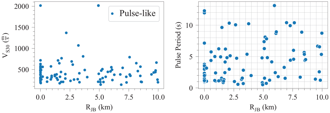
To simulate strong ground motions from the February 6, 2023, Kahramanmaraş, Türkiye, earthquake (Mw = 7.8), hereafter referred to as the Kahramanmaraş earthquake, we select a dataset of recorded motions with Joyner-Boore distances (RJB) less than 80 km from the pan-European strong-motion (ESM) database (Luzi et al., 2016). Figure 1 shows the frequency distribution of the 41 selected recording pairs (82 components in the as-recorded directions) with respect to RJB and the averaged shear wave velocity at the top 30 m of soil (VS30). The selected records encompass a wide range of source-to-site distances and soil conditions. Wu et al. (2023) identified 18 pairs of these recordings as pulse-like motions, using the pulse index value at the orientation of the largest pulse determined through Baker’s algorithm (Baker, 2007). Figure 2 shows a scatter plot of VS30 versus RJB, distinguishing pulse-like and non-pulse-like motions, along with the period of the largest pulse for the identified pulse-like motions. Four sample time-series in the north-south (NS) and east-west (EW) directions are shown in Figure 3, showing a diverse set of characteristics, including pulse-like, non-pulse-like, single, and double strong phase motions at different source-to-site rupture distances.
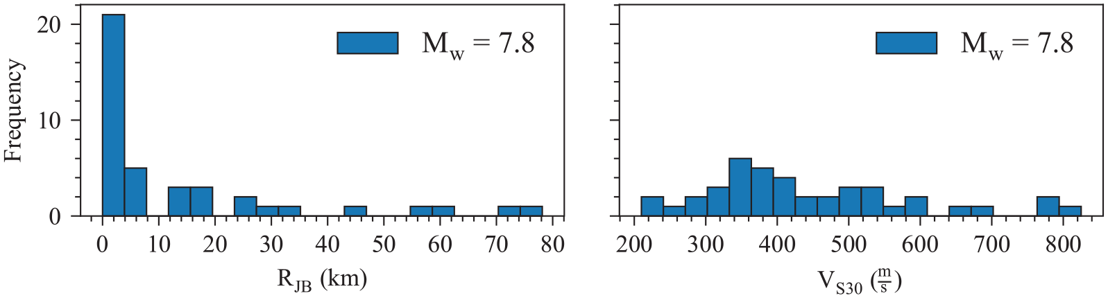
Frequency distribution of the selected ground motions from Kahramanmaraş, Türkiye, earthquake with moment magnitude (Mw) 7.8, with respect to Joyner-Boore distance (RJB) and averaged shear wave velocity at the top 30 m of soil (VS30).
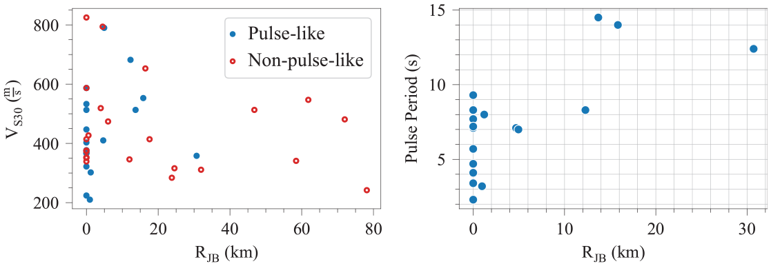
Scatter plot of VS30 versus RJB for the Kahramanmaraş, Türkiye, earthquake dataset (Luzi et al., 2016), distinguishing pulse-like and non-pulse-like motions, along with the pulse period values for the identified pulse-like motions.
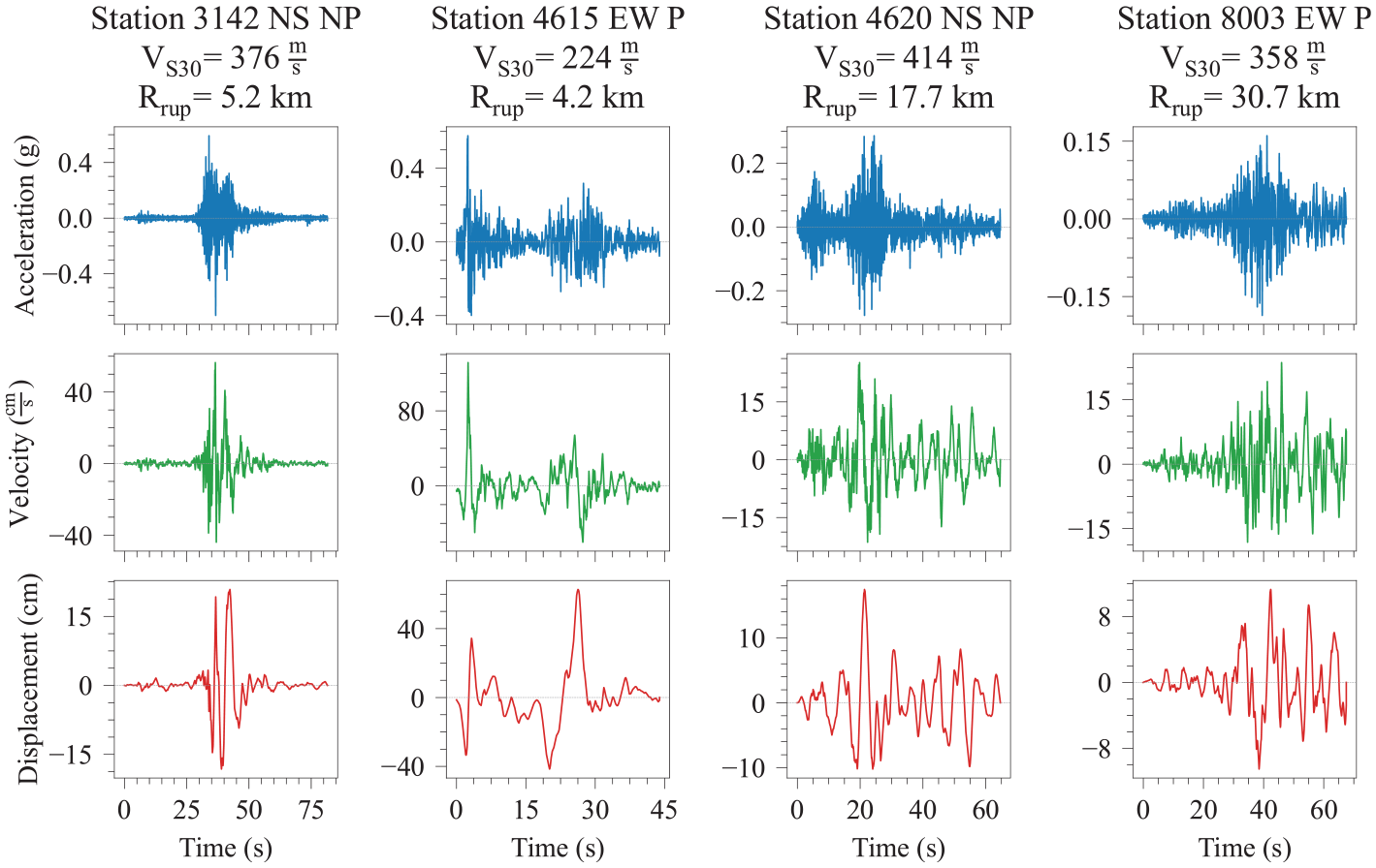
Sample ground motion time-series from the Kahramanmaraş, Türkiye, earthquake dataset (Luzi et al., 2016), at various VS30, source-to-site rupture distances (Rrup), showing pulse-like (P), non-pulse-like (NP), single (left and right panels), and double strong-phase motions (mid panels).
To assess the ability of the improved model to accurately represent low-frequency pulse-like ground motions for a range of earthquake magnitudes, a subset of the NGA-West2 database (Ancheta et al., 2014) is also selected. This subset includes 97 recording pairs (194 components) of pulse-like motions with RJB less than 10 km, selected without additional assumptions. Figure 4 shows the frequency distribution of the selected motions across RJB, VS30, and Mw, and Figure 5 shows a scatter plot of VS30 versus RJB, along with estimated values of pulse periods for each motion as calculated by Shahi and Baker (2014) and reported in the NGA-West2 database.
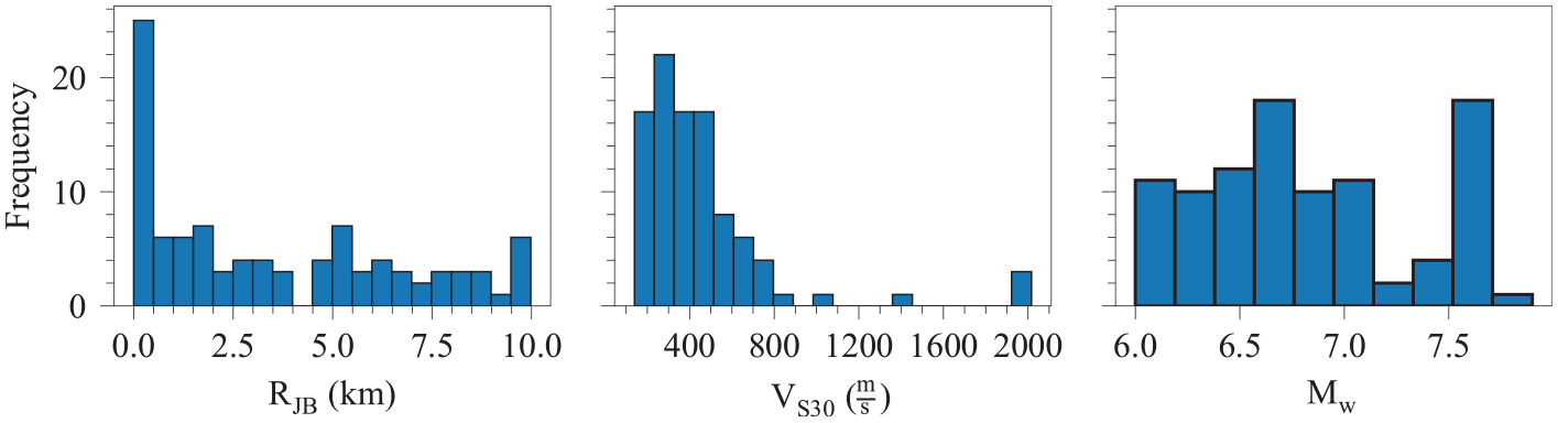
Frequency distribution of the selected ground motions from the Next Generation Attenuation Relationships for Western United States (NGA-West2) dataset (Ancheta et al., 2014), with respect to RJB, VS30, and Mw.
Scatter plot of VS30 versus RJB for the selected pulse-like NGA-West2 dataset (Ancheta et al., 2014), along with the pulse period values of the motions.
The combined Kahramanmaraş earthquake and NGA-West2 datasets result in a total of 276 representative ground motion components, sourced from various regions and earthquakes. Information about the selected records regarding the ESM (https://esm-db.eu) and NGA-West2 (https://ngawest2.berkeley.edu/site) databases is summarized in Supplementary Table A2.1 and Table A2.2, respectively.
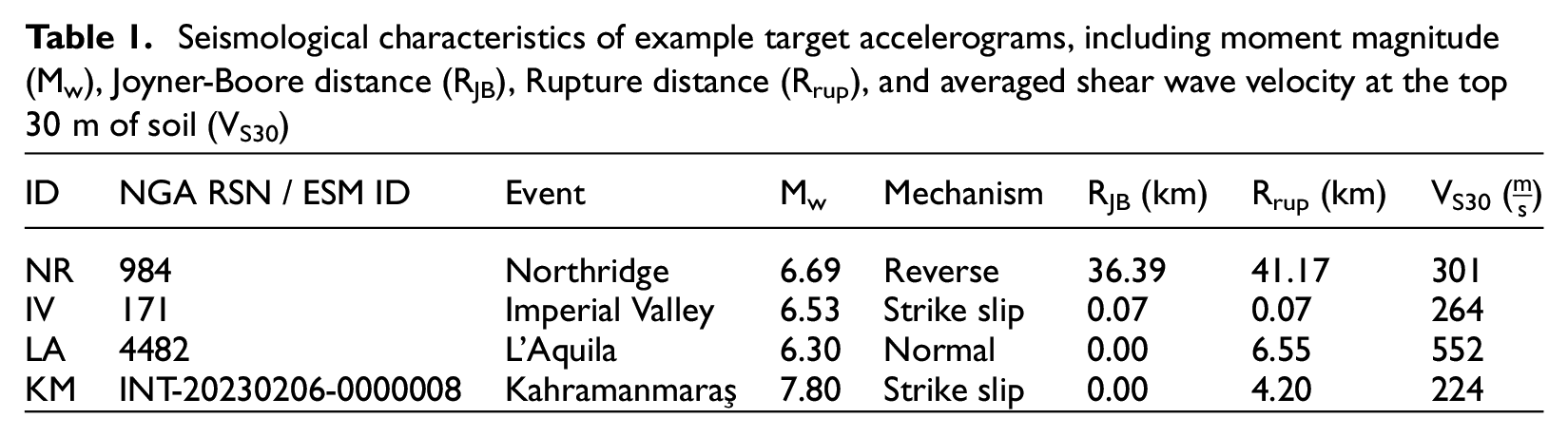
The four accelerograms, shown in Table 1, are selected for illustrative purposes and discussions in this study. These example accelerograms include the non-pulse-like component 90 of the Northridge-01 1994 (United States) earthquake recorded at the 116th Street School station with record sequence number (RSN) of NGA RSN 984, the pulse-like component 0 of the Imperial Valley-06 1979 (United States) earthquake recorded at El Centro-Meloland Geotechnical Array station (NGA RSN 171), the pulse-like horizontal EW component of the L’Aquila 2009 (Italy) earthquake recorded at station L’Aquila-V.Aterno-F. Aterno (NGA RSN 4482), and the pulse-like horizontal EW component of the Kahramanmaraş 2023 (Türkiye) earthquake recorded at station 4615 (ESM ID INT-20230206-0000008). The latter two accelerograms exhibit double strong-motion phases. In this study, an identifier (ID) is assigned to each target recorded ground motion for ease of reference, as shown in Table 1.
Seismological characteristics of example target accelerograms, including moment magnitude (Mw), Joyner-Boore distance (RJB), Rupture distance (Rrup), and averaged shear wave velocity at the top 30 m of soil (VS30)
The stochastic ground motion model
The reference model
This study builds upon the site-based stochastic model developed by Rezaeian and Der Kiureghian (2008). This reference model accounts for both the temporal and spectral non-stationarities of earthquake ground motion time-series. One of the key benefits of this model is the ease of parameter estimation, achieved by separating the temporal and spectral non-stationary features of the stochastic process. The ground acceleration process
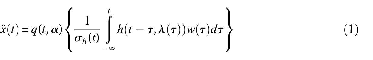
where

where
The model formulation in Equation 1 and the corresponding high-pass filter in Equation 2 have served as the basis for the development of several improved non-stationary site-based stochastic models in the literature. These models have primarily aimed to broaden the applicability range of the model by enhancing its low-frequency content representation either by incorporating a deterministic forward directivity velocity pulse model or by refining the filter through sequential filtering techniques (e.g. Dabaghi and Der Kiureghian, 2017; Waezi and Balzadeh, 2022; Waezi et al., 2021). Moreover, the evolutionary frequency content of a ground motion time-series is affected by several factors, including the characteristics of the earthquake source, path, and site. These intricate non-stationary processes demonstrate multiple peak frequencies in their evolutionary PSDs. To better characterize this spectral non-stationarity, several studies have assumed two or three peak frequencies and corresponding bandwidths at the expense of additional parameters and complexity (Vlachos et al., 2016; Waezi and Balzadeh, 2022; Waezi et al., 2021). However, direct identification of multiple evolutionary peak frequencies is not straightforward and often requires non-stationary spectral estimation techniques such as short-time Fourier transform (Vlachos et al., 2016; Waezi and Balzadeh, 2022).
The limitations
The reference model in Equation 1, with the application of the high-pass filter in Equation 2, exhibits two main limitations. First, there could be a total energy deficit in the final process due to the high-pass filtering, and although this bias was negligible for the applicability range of the original records considered by Rezaeian and Der Kiureghian (2008), it could be noticeable for records that are near-fault or on deep basins and exhibit lower-frequency contents. Although the residual velocity and displacement are removed through a stationary high-pass filter, this post-processing step can eliminate a part of the low-frequency contents and the corresponding energy from the simulations. Thus, the final process can systematically underestimate the total energy with respect to the initial process. In the validation studies done by Rezaeian and Der Kiureghian (2008, 2012), such underestimations were considered nonsignificant for the selected set of strong far-field recorded ground motions; however, they may be of considerable interest in ground motions where a substantial portion of the energy comes from low-frequency contents, such as those observed in some of the records in the Kahramanmaraş earthquake.
Several studies have incorporated a stationary high-pass filter as a part of the main filter function within the reference model (Broccardo and Dabaghi, 2019; Waezi and Balzadeh, 2022; Waezi et al., 2021) or an evolutionary power spectral-based model (Vlachos et al., 2016). Although this inclusion may alleviate excessive low-frequency contents in the final process, several challenges persist. First, determining the optimal high-pass frequency parameter remains ambiguous, often requiring iterative adjustments to the parameter to achieve realistic velocity and displacement time-series (Rezaeian and Der Kiureghian, 2008; Vlachos et al., 2016), which has some degree of subjectivity. In a recent study (Su et al., 2024), this stationary high-pass corner frequency was optimized by matching the long-period (T ≥ 1 s) linear acceleration response spectrum of synthetic ground motions to that of each target record. Second, the implementation of a stationary high-pass filter is susceptible to generating undesired response amplitudes near its frequency parameter due to the cumulative effect of response contributions in the integral term in Equation 1. Consequently, a high-pass filter that attenuates frequencies below a stationary corner frequency, uniformly across all time instances, may be inadequate for simulating ground motions in which an important part of the non-stationary frequency content lies within the low-frequency range, such as in near-fault pulse-like motions and motions with deep basin effects.
As the second limitation, time-modulating after filtering a process as highlighted by Safak and Boore (1988) distorts the low-frequency content in the Fourier amplitude spectrum (FAS) of the process. This latter limitation indicates that models based on Equation 1, despite incorporating a stationary high-pass filter, could still require an additional post-simulation high-pass filtering. Consequently, this results in an inherent bias in the total energy, requiring a post-simulation energy correction factor to address the induced bias as described by Dabaghi and Der Kiureghian (2017) and Broccardo and Dabaghi (2019). Similarly, site-based stochastic models are typically fitted to target records based on criteria such as the rates of zero-level crossings and counts of local extrema. However, post-simulation high-pass filtering can introduce bias, causing the simulations to deviate from the original fitting criteria.
These two limitations restrict the application of the reference model to only far-field ground motions and motions without the presence of deep basin effects, in which low-frequency contents do not contribute to a substantial portion of the total energy. To broaden the applicability range of the reference model to near-fault pulse-like motions, previous studies have used a deterministic forward directivity velocity pulse model (Dabaghi and Der Kiureghian, 2017; Waezi and Balzadeh, 2022). This approach involves several steps to first identify and extract the largest pulse using a wavelet-based method, as outlined in Baker’s algorithm (Baker, 2007), and then, a forward directivity velocity pulse model would be fitted to the extracted pulse in the velocity domain. The derivative of this model is then combined with a stochastic model of the residual motion, tailoring it to cases of forward directivity velocity pulses.
The proposed improved stochastic model
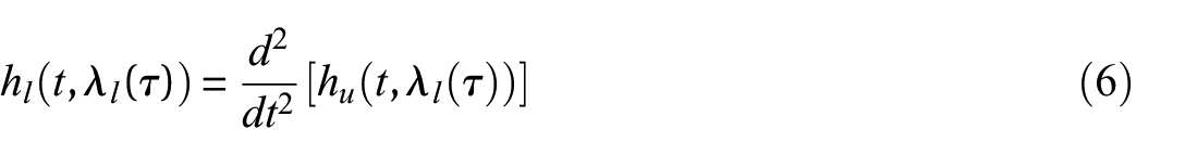
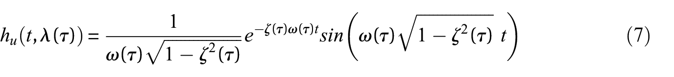
In this study, we first modify the order of time-modulating and filtering in the formulation of the reference model. The proposed modification is based on band-pass filtering of a time-modulated Gaussian white noise process. The band-pass filter is selected based on the response of a linear time-variant (LTV) SDoF system. Following the same terminology as the reference model, we define the IRF of the LTV filter as
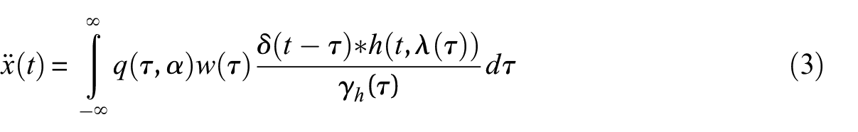
where
It is important to note that the term inside the integral in Equation 3 is a stationary Gaussian process at each instance of
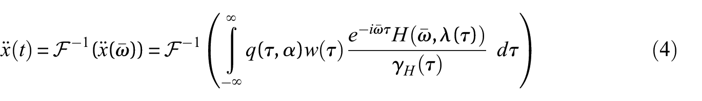
where
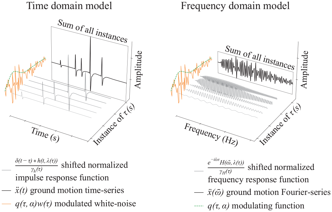
Schematic representation of the improved stochastic model in the time and frequency domains.
The proposed filter function
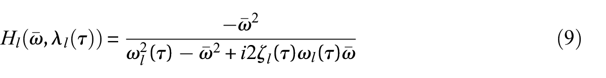
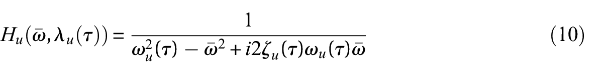
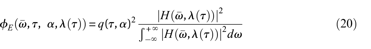
For the filter function, we use the FRF of the filter

where subscripts
where

here,
The functional forms of the filter parameters
where
The proposed time-modulating function
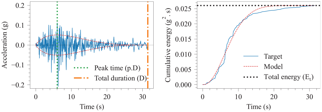
Existing time-modulating functions include the piecewise function (Amin and Ang, 1968; Housner and Jennings, 1964), the double-exponential function (Shinozuka and Sato, 1967), and the Gamma function (Rodolfo Saragoni and Hart, 1973). Stafford et al. (2009) proposed a modulating function based on the Lognormal distribution, which models the energy buildup in ground motion time-series. These parameterized time-modulating functions describe the arrival of energy in a single strong phase, preceded by an energy buildup and followed by a decay, which may not necessarily reach zero at the end of the acceleration process. Consequently, for accelerograms characterized by the arrival of energy in multiple strong phases, these functions require adjustments. Figure 7 illustrates an example of such ground motions, featuring the Kahramanmaraş (KM) accelerogram (refer to Table 1) along with a corresponding fitted Gamma function as used by Rezaeian and Der Kiureghian (2010). Notably, the fitted Gamma function is unable to capture the realistic arrival of energy.
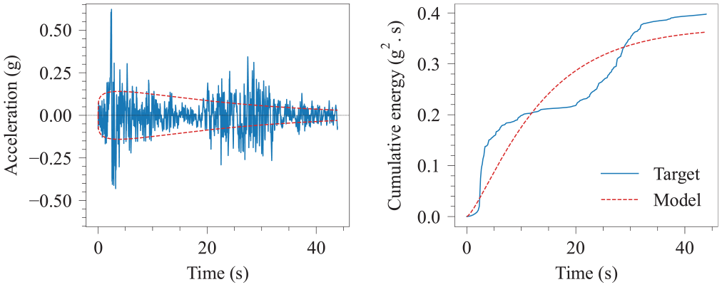
The Kahramanmaraş accelerogram with multiple strong phases, along with the fitted Gamma function and their cumulative energy.
Moreover, existing time-modulating functions rely on mathematical parameters that often lack physical interpretation. One way to relate these parameters to the seismological characteristics of a scenario earthquake is through empirically developed predictive models (Rezaeian and Der Kiureghian, 2010; Stafford et al., 2009). Modulating functions often require adjustments to account for various shapes of ground motion time-series, such as near-fault pulse-like accelerograms, by introducing additional parameters in the function (e.g. Dabaghi and Der Kiureghian, 2017). Numerical interpolation methods like monotonic cubic Hermite splines can require a varying number of input parameters depending on the target motion and desired accuracy. Broccardo and Dabaghi (2019) recommended using seven interpolation points to model the modulating function. These numerical methods may necessitate supplementary post-processing to achieve a smooth modulating function and circumvent issues like overshooting (e.g. a local abrupt jump), particularly when neighboring interpolation points are spaced very closely. This can be challenging for recorded motions with rapid energy arrivals, requiring a choice of interpolation points based on the specific characteristics of the motion.
To overcome the limitations of existing time-modulating functions, here we use concave Beta distributions to describe the energy buildup in ground motions. Let
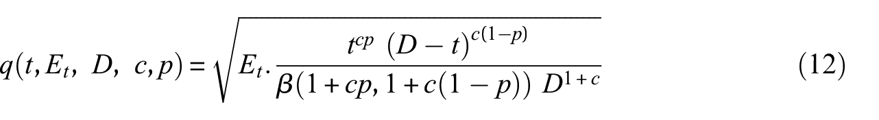
where p is the ratio of the time of peak amplitude to the total duration (i.e.
Parameters of the basic beta function fitted to the Northridge accelerogram.
The arrival of energy in multiple strong phases can be replicated by a weighted sum of basic Beta time-modulating functions. The proposed Beta modulating function which explicitly starts from and ends in zero amplitude, can be expressed as follows:
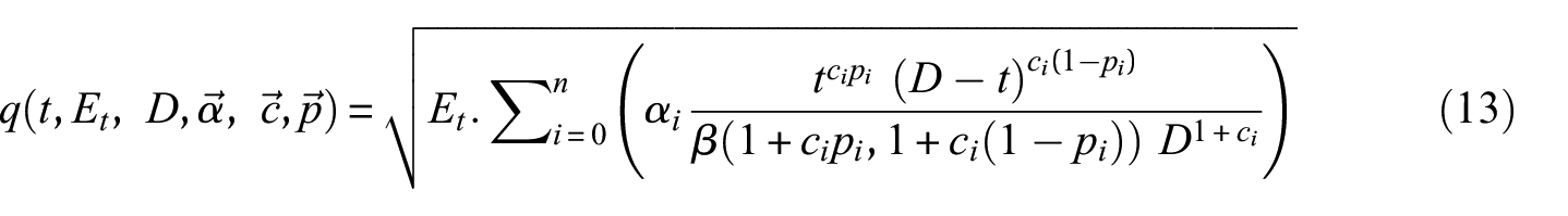
where
Therefore, the improved stochastic model is fully defined by eight parameters (
Fitting to the evolutionary frequency and energy contents of the ground motion process
Time-varying frequency content
To characterize the predominant frequency and bandwidth, many site-based stochastic models have used the rate of zero-level up-crossings and positive-minima and negative-maxima of the acceleration process, respectively (e.g. Dabaghi and Der Kiureghian, 2017; Rezaeian and Der Kiureghian, 2008; Rodolfo Saragoni and Hart, 1973; Waezi et al., 2021; Yeh and Wen, 1990). To explore the characteristics of a ground motion time-series, we define mean zero crossing (MZC), mean local extrema (MLE), and mean positive-minima and negative-maxima (MPMNM) as follows; MZC represents the average number of zero-level up-crossings and down-crossings, MLE denotes the average number of local minima and maxima, and MPMNM indicates the average number of local positive-minima and negative-maxima. Analysis of these three features within recorded ground motions demonstrates that the MZC of acceleration equals the MLE of velocity, and the MZC of velocity equals the MLE of displacement, which is supported by the theoretical definitions of acceleration, velocity, and displacement processes. Similarly supported by their definitions, the MPMNM of velocity is half of the difference between its MLE and MZC. Likewise, the MPMNM of displacement is half of the difference between its MLE and MZC. Figure 9 illustrates these relationships for the example NR ground motion (refer to Table 1).
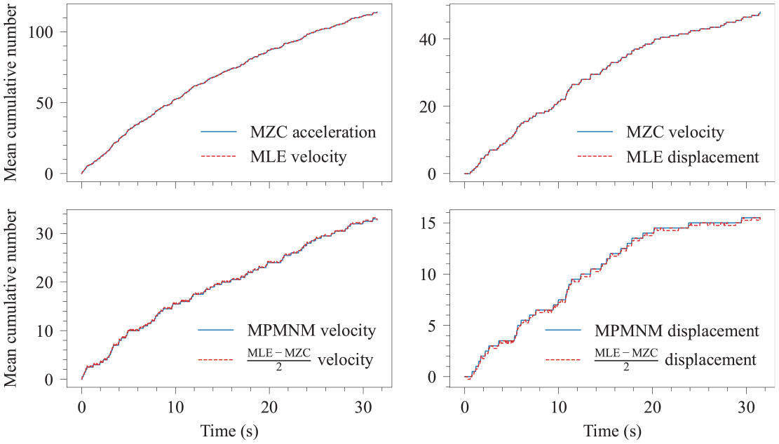
Relationships between time-series characteristics of recorded ground motions, using the Northridge accelerogram. Characteristics include mean zero crossing (MZC), mean local extrema (MLE), and mean positive-minima and negative-maxima (MPMNM).
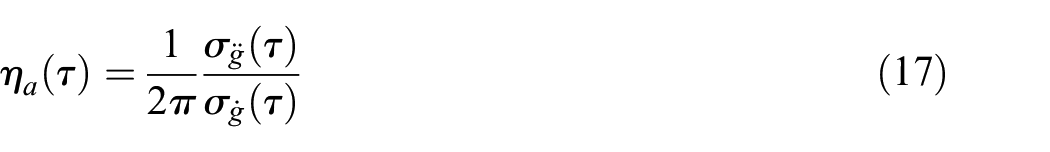
As such, the MPMNM of a process can be replaced with the difference between the MZC of that process and its time-derivative. In other words, given that the MZC of a process (i.e. acceleration, velocity, or displacement) is related to its dominant frequencies, the MPMNM of the process is associated with the bandwidth between the dominant frequencies of that process and its time-derivative. Therefore, the MZC of acceleration, velocity, and displacement processes can be used as proxies for high, intermediate, and low dominant frequencies, respectively. Similarly, the MPMNM of the displacement and velocity processes can be used as proxies for the bandwidth between low to intermediate and intermediate to high dominant frequencies. As the MPMNM of the acceleration process acts as a proxy for the bandwidth between the acceleration and its time-derivative, it may not provide any advantages for modeling the acceleration, velocity, and displacement time-series. Consequently, it is not used as a fitting criterion in this study. Subsequently, we formulate these features for the acceleration, velocity, and displacement processes of the stochastic model.
Let
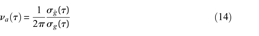
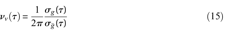
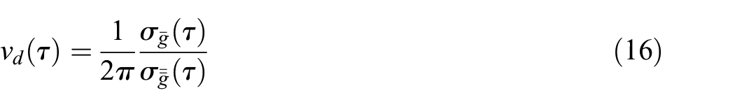
where
where
This study uses Equations 14–16 as the fitting criterion to describe the time-varying frequency content of a target recorded motion. As a result, the MZC of acceleration and displacement processes serve as proxies for the upper and lower dominant frequencies, respectively. To avoid redundancy, the MZC of the velocity process (alongside acceleration and displacement MZC) adequately accounts for the bandwidth of the process, implicitly capturing the MPMNM of the velocity and displacement processes.
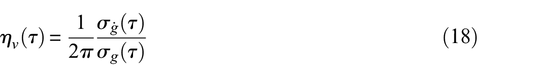
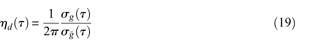
In Equation 3, the term
Therefore, the variance of the process
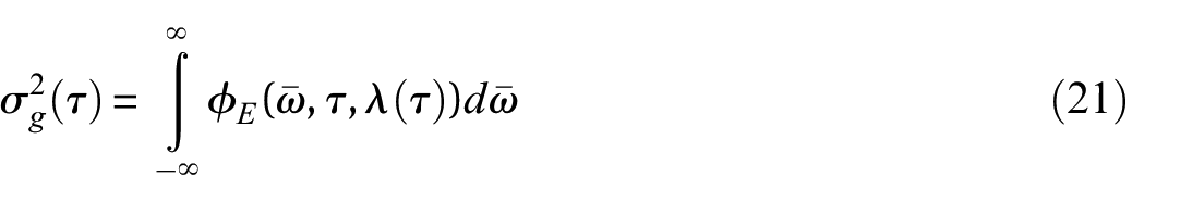
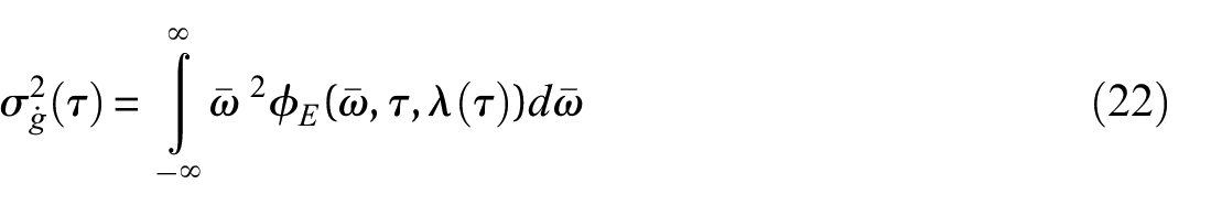
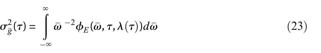
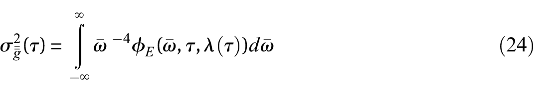
Because
Time-varying energy content
Fitting to the time-varying energy content follows the same procedure used by Rezaeian and Der Kiureghian (2008) but with an added number of parameters for the time-modulating function. For a ground motion time-series
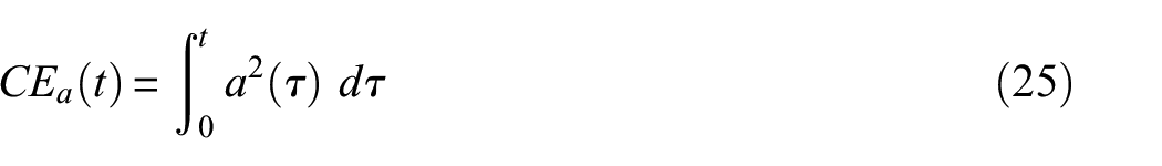
Similarly, the expected CE of the process
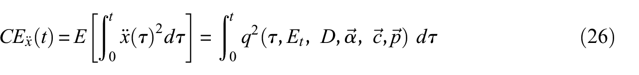
This means the modulating function can fully and independently describe the energy content of the process.
Parameter identification
Similar to Rezaeian and Der Kiureghian (2008), the parameters of both the filter and the time-modulating function can be independently identified by matching the characteristics outlined in the previous section with those of a target accelerogram. Unlike Rezaeian and Der Kiureghian (2008), in which filter parameters were identified by matching to the MZC and MPMNM of the acceleration process, we identify the parameters by matching to the MZC of the acceleration, velocity, and displacement processes. This adjustment to the objective functions is necessary to converge to an optimized set of model parameters given their increased number and is more intuitive given their segregation into lower and upper limits of the dominant frequency in Equations 9–10.
Parameter identification for the filter function
The filter parameters (
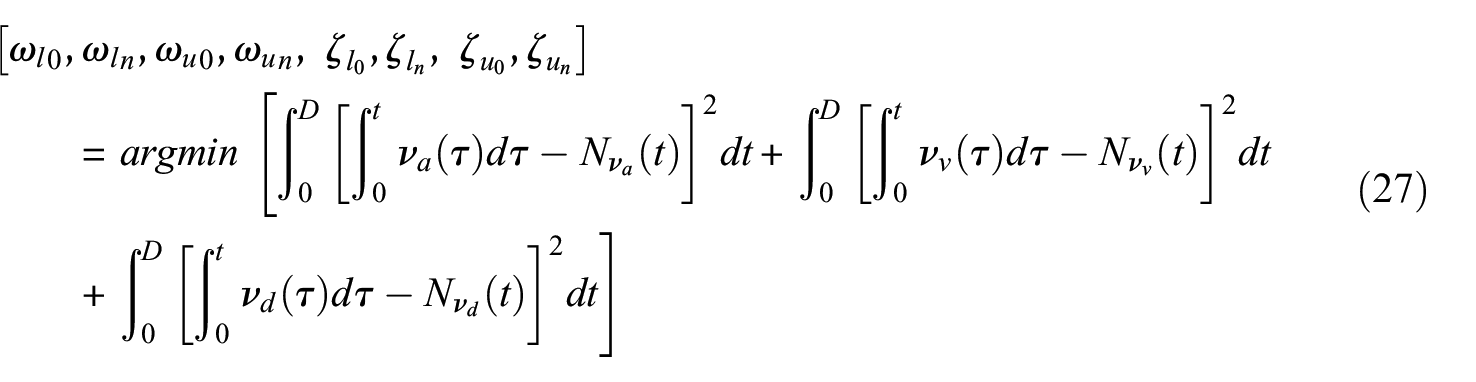
where
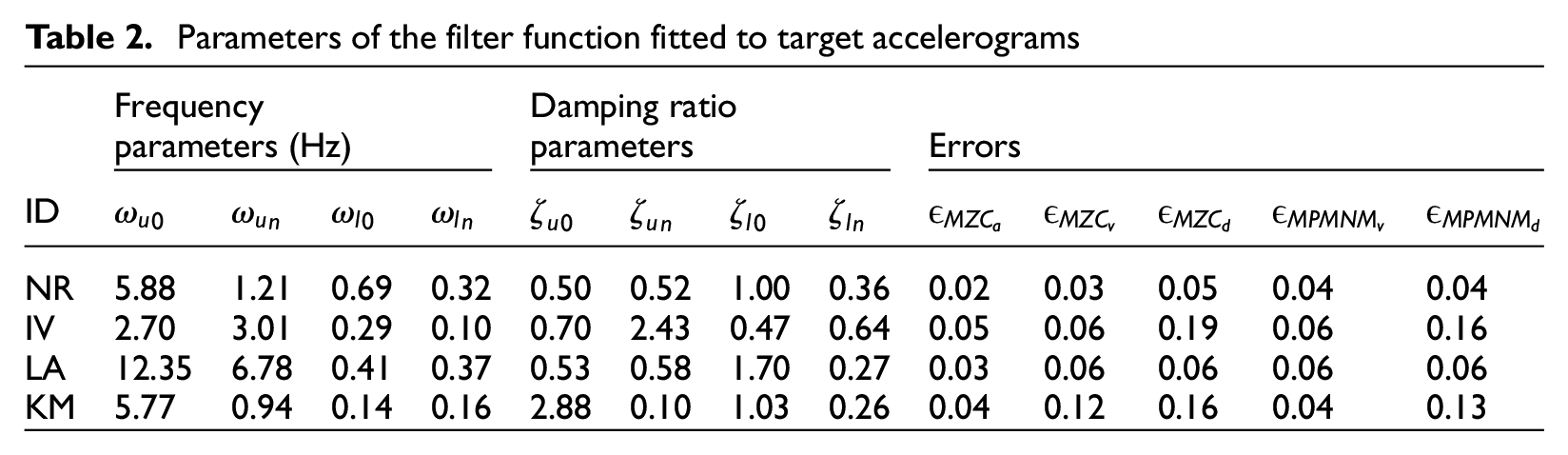
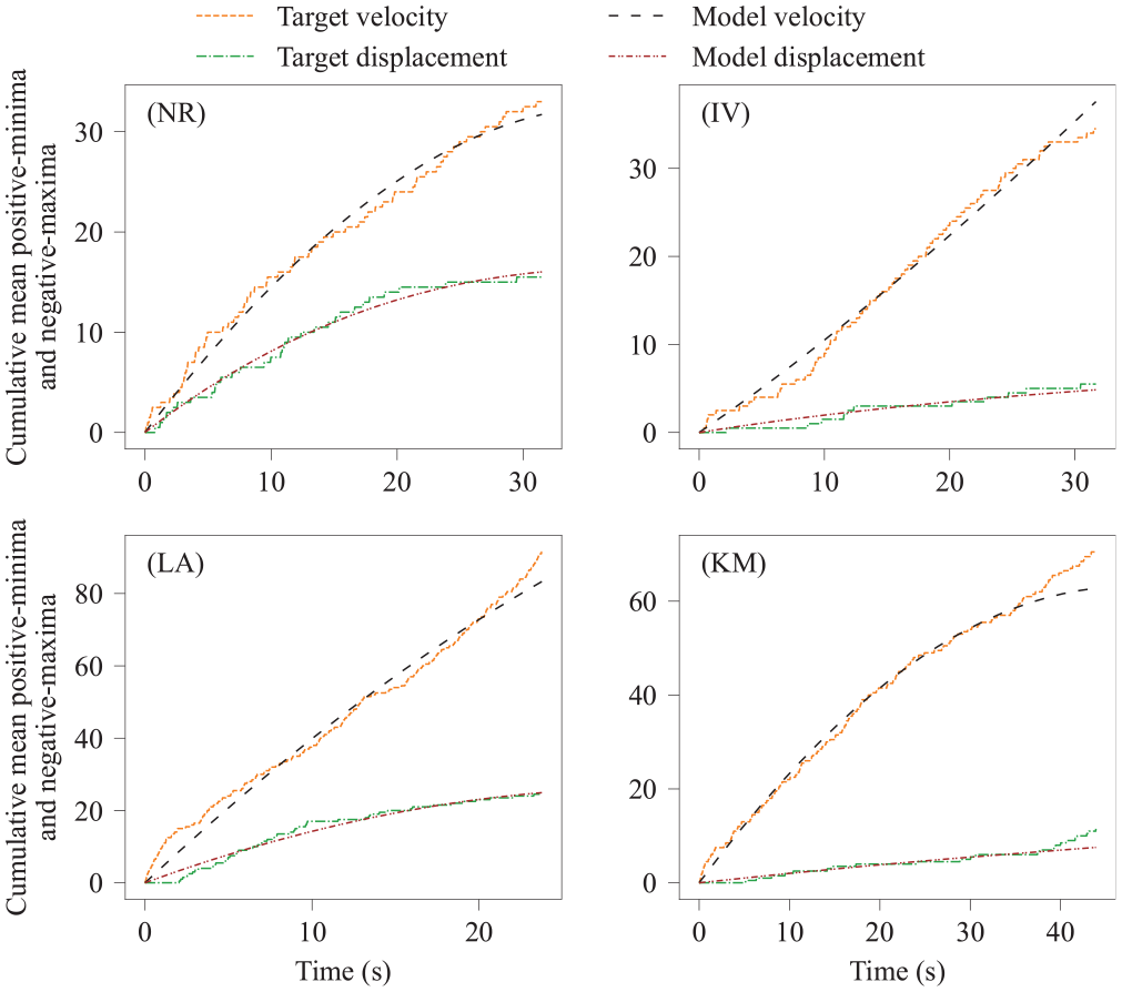
Figure 10 illustrates the cumulative MZC of the example target accelerograms, their velocity and displacement time-series, and the corresponding fitted models. Identified filter parameters are shown in Table 2. The MZC rate of the target motions (i.e. acceleration, velocity, and displacement), which is the slope of the corresponding curves in Figure 10, fluctuates over time for all selected accelerograms. This means that the dominant frequencies in the target motions vary with time. In the case of the Imperial Valley (IV) (refer to Table 1) accelerogram with a shorter rupture distance (Rrup = 0.07 km) and a soft soil (VS30 = 264
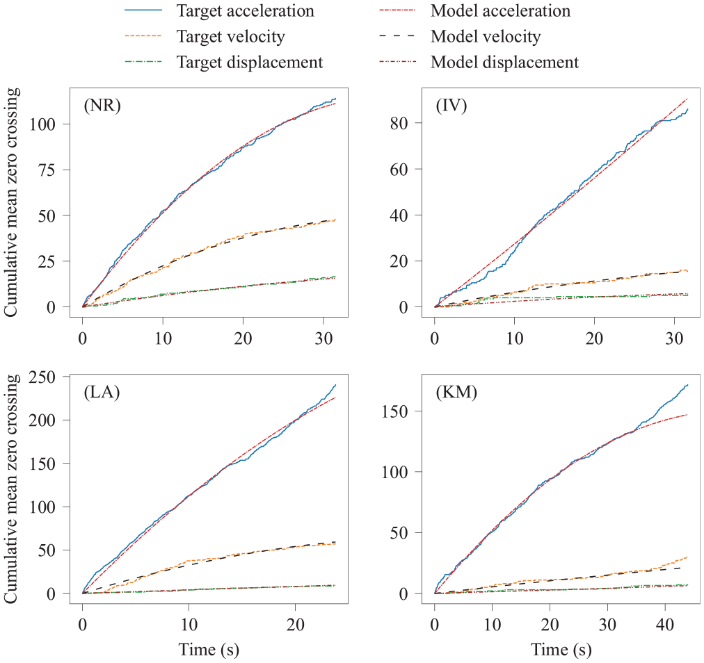
Cumulative mean zero crossings of the target acceleration, velocity, and displacement time-series, along with their corresponding fitted models. The panels correspond to Northridge (NR), Imperial Valley (IV), L’Aquila (LA), and Kahramanmaraş (KM) ground motions.
Parameters of the filter function fitted to target accelerograms
Cumulative mean positive-minima and negative-maxima of the target velocity and displacement time-series, along with their corresponding fitted models. The panels correspond to Northridge (NR), Imperial Valley (IV), L’Aquila (LA), and Kahramanmaraş (KM) ground motions.
Errors for various validation metrics (e.g. MZC of acceleration) can be calculated using the following expression:
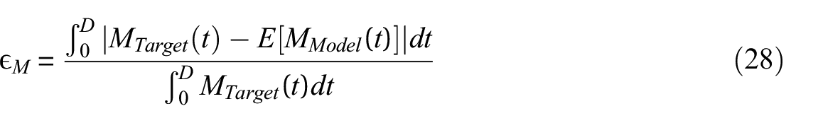
where M refers to the relevant validation metric for both the target and expected model processes, and
Parameter identification for the time-modulating function
The parameters of the time-modulating function (
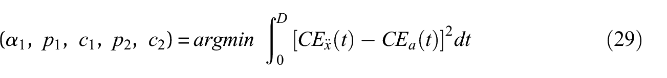
To ensure a unique solution for cases with two strong phases, it is assumed that the first phase precedes the second, imposing the constraint
Recorded ground motions often exhibit leading or trailing zeros or negligible amplitudes, resulting in different durations. To avoid these tails that have a negligible contribution to the total energy, the target motion is defined as that corresponding to 0.1%–99.9% of the total energy of the input recorded accelerogram. Figure 12 illustrates the target motion and the corresponding duration for LA as an example (refer to Table 1).
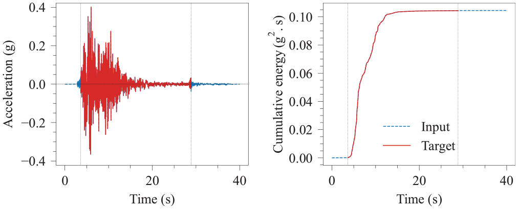
The L’Aquila (LA) target motion corresponding to 0.1%–99.9% of the total energy of the input LA accelerogram.
Errors associated with CE are determined by substituting CE for the variable M in Equation 28. The identified parameters of the modulating function and the corresponding errors are shown in Table 3. Figure 13 illustrates the modulating function and CE of the model when fitting to the corresponding target accelerograms. The fit with slight error demonstrates the capability of the time-modulating function in modeling various shapes of ground motions, including pulse-like and double strong phase motions. The arrival of energy in a single strong phase is observable in NR and IV with a more abrupt arrival in the latter (refer to Table 1). In NR, 76.6% of the total energy is smoothly distributed around the first peak time (
Parameters of the modulating function fitted to target accelerograms
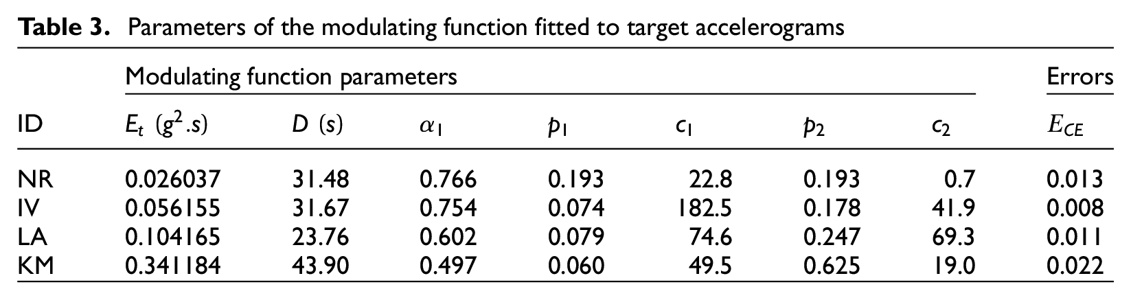
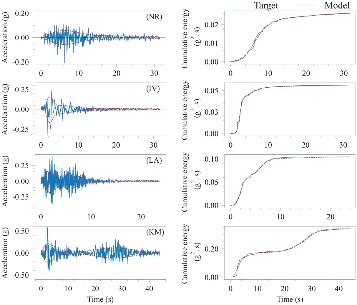
Fitted modulating function to target accelerograms and their respective cumulative energy. The panels correspond to Northridge (NR), Imperial Valley (IV), L’Aquila (LA), and Kahramanmaraş (KM) ground motions.
Validation
Before simulations can be used in engineering applications, it is crucial to thoroughly validate the simulation methodologies and their outcomes by assessing their effectiveness in predicting both seismological and engineering demand parameters (Karimzadeh, 2019; Rezaeian et al., 2024; Smerzini et al., 2024). Such validation ensures that the model accurately represents the main characteristics of recorded ground motions, thus demonstrating the reliability of the synthetic motions for engineering applications. Validation procedures in the literature are often based on characteristics that are expected to affect engineering systems, such as elastic response spectra or other ground motion validation metrics (Arslan Kelam et al., 2022; Askan et al., 2017; Burks and Baker, 2014; Goulet et al., 2015; Karimzadeh et al., 2020, 2023, 2024a; Olsen and Mayhew, 2010; Rezaeian and Der Kiureghian, 2010). In this study, we first perform a visual comparison between the ground motion time-series, CE, Fourier amplitude, and elastic response spectra of the four example target accelerograms and those of simulations generated from the fitted stochastic model parameters described in previous sections. Next, we quantitatively assess the efficiency of the improved stochastic model using 276 horizontal components from the selected datasets.
Visual qualitative comparisons of target and simulated motions
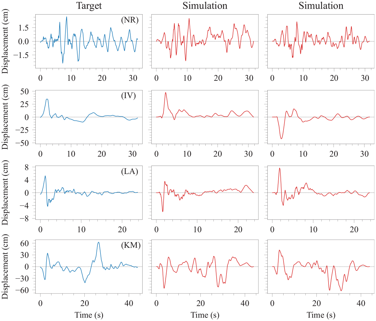
Given the identified model parameters in the previous section, the improved stochastic model can directly simulate ground motion time-series without added deterministic components or any additional post-processing. Figures 14–16 show the acceleration, velocity, and displacement time-series for the four example target motions listed in Table 1, along with two realizations for each, obtained from stochastic simulations as described in previous sections. In Figure 14, the stochastic simulations resemble target accelerograms in terms of the overall waveforms, intensity levels, durations, and frequency contents. In particular, simulations of LA and KM exhibit multiple strong phases like their respective target motions. This illustrates the effectiveness of the proposed modulating function in accurately accounting for the arrival of energy in multiple strong phases. The simulated velocity time-series in Figure 15 are also like those of target motions, capturing the overall waveforms, pulse timings, and pulse intensities without considering additional explicit constraints on these features. For example, in IV, a velocity pulse is observed at
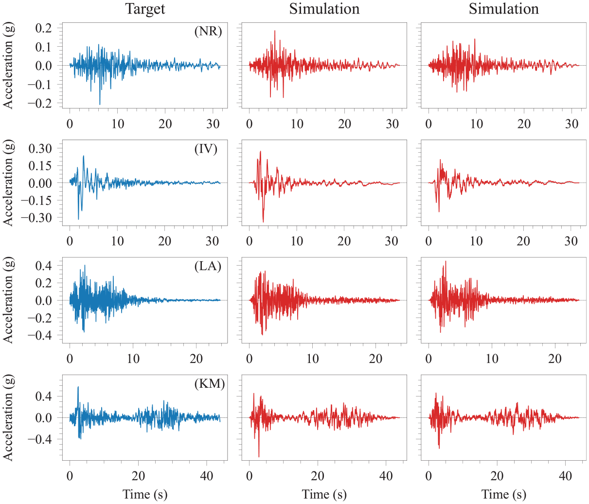
Target accelerograms and two alternative simulations using the corresponding fitted models. The panels correspond to Northridge (NR), Imperial Valley (IV), L’Aquila (LA), and Kahramanmaraş (KM) ground motions.
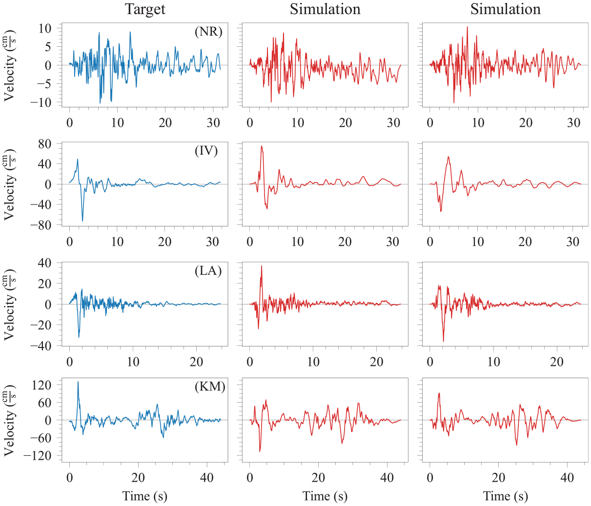
Velocity time-series and two alternative simulations using the corresponding fitted models. The panels correspond to Northridge (NR), Imperial Valley (IV), L’Aquila (LA), and Kahramanmaraş (KM) ground motions.
Displacement time-series and two alternative simulations using the corresponding fitted models. The panels correspond to Northridge (NR), Imperial Valley (IV), L’Aquila (LA), and Kahramanmaraş (KM) ground motions.
Figure 17 shows the CE of the target accelerograms and 20 random realizations from simulations. CEs of the target accelerograms lie within one standard deviation of the corresponding simulated motions. This indicates that the target accelerogram can be regarded as one reasonable realization of the stochastic model. It is noteworthy that CE is non-linear with respect to the amplitude of each simulation, and the amplitude is influenced by the random component of modulated white noise,
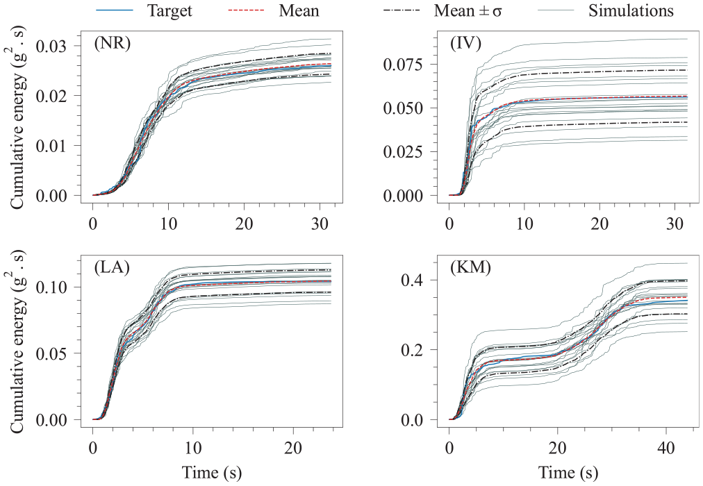
Cumulative energy of the target accelerograms and 20 random simulations using the corresponding fitted models. The panels correspond to Northridge (NR), Imperial Valley (IV), L’Aquila (LA), and Kahramanmaraş (KM) ground motions. The standard deviation is denoted as
For further comparison, the FAS and 5%-damped response spectral acceleration (SA) for the target accelerograms and 20 random realizations from their simulations are shown in Figures 18 and 19, respectively. The FAS is smoothed using a simple moving average with a window size of 9 points solely for visual comparison. FAS for simulations can be represented directly using Equation 4. The FAS and SA of the target motions fall within the ranges spanned by those of the simulated motions nearly across all frequency and period ranges. Therefore, the target motions can be considered reasonable realizations of the stochastic model for the given parameters. The rather smooth shape of the mean FAS and SA is attributed to the linear functional form of filter parameters, aiming to capture evolutionary dominant frequencies and bandwidth parameters in an average manner. Consequently, the linear functions do not capture all local fluctuations of these parameters. For instance, in the IV, a local peak in SA is evident around the period of 0.7 s, and the mean SA does not exhibit this distinct peak. Yet, such peaks occur within the range of simulations due to the variability. Nevertheless, given the intricate nature of ground motions, different functional forms can be used to represent the very local variation of these filter parameters. However, this is not pursued in this study and will likely lead to more parameters and more complex models.
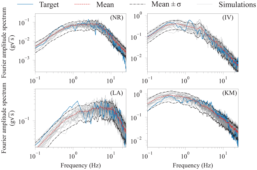
Fourier amplitude spectrum of the target accelerograms and 20 alternative simulations using the corresponding fitted models. The panels correspond to Northridge (NR), Imperial Valley (IV), L’Aquila (LA), and Kahramanmaraş (KM) ground motions. The standard deviation is denoted as
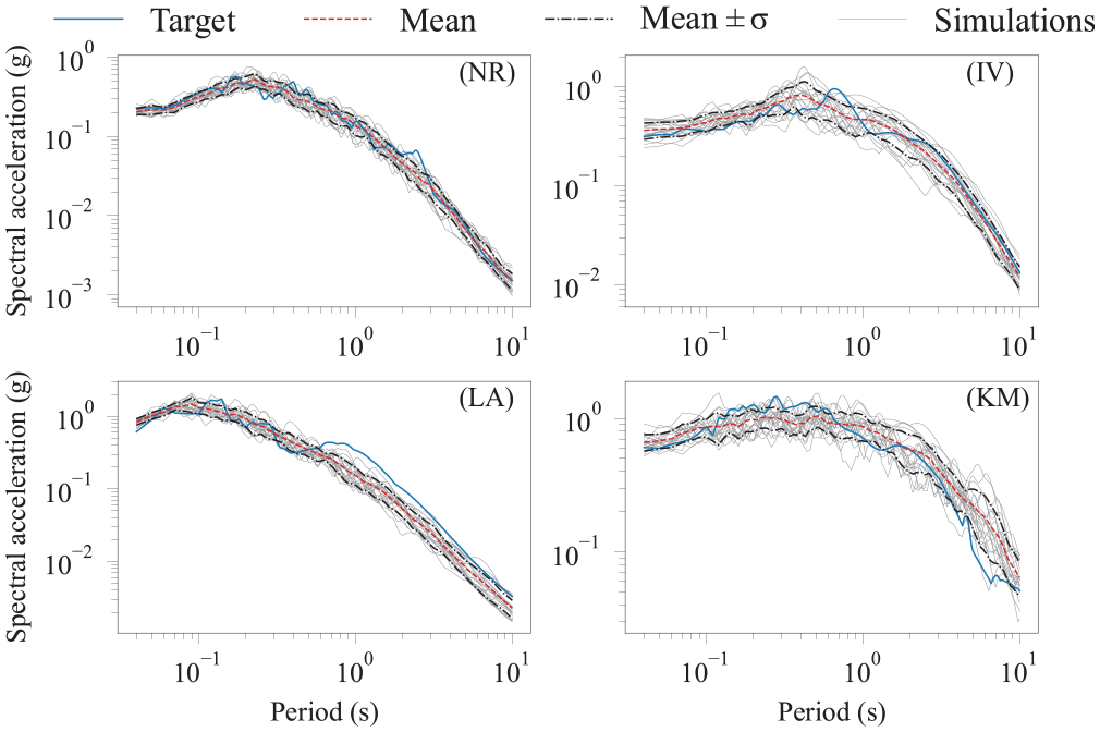
Spectral acceleration of the target accelerograms and 20 alternative simulations using the corresponding fitted models. The panels correspond to Northridge (NR), Imperial Valley (IV), L’Aquila (LA), and Kahramanmaraş (KM) ground motions. The standard deviation is denoted as
Next, quantitative error measures for the FAS (
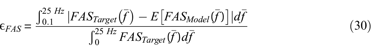
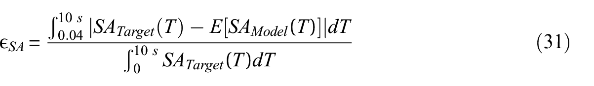
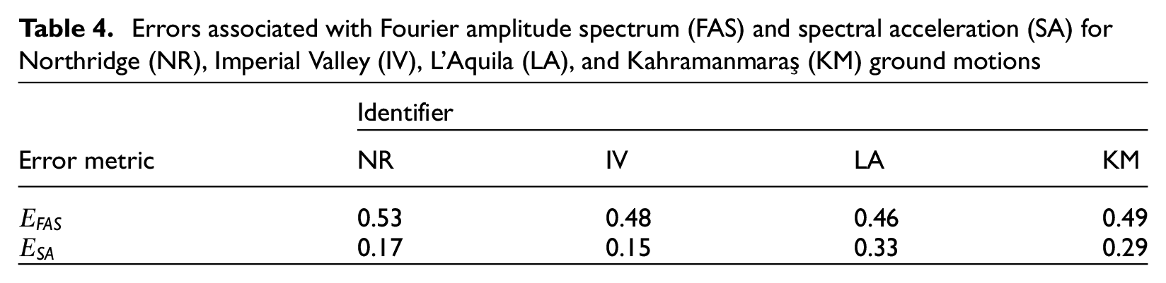
These errors are reported in Table 4, and alongside error measures in previous sections, they can provide an understanding of the relationship between the quantitative errors and visual assessments. These errors exhibit increased values due to the abrupt amplitude variations in the target FAS and SA. Nonetheless, based on visual assessment, the simulation model effectively captures the overall behavior.
Errors associated with Fourier amplitude spectrum (FAS) and spectral acceleration (SA) for Northridge (NR), Imperial Valley (IV), L’Aquila (LA), and Kahramanmaraş (KM) ground motions
Quantitative model evaluation for the selected datasets
Empirical cumulative distribution function of errors
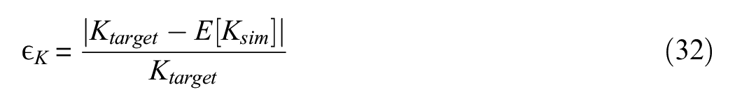
Quantitative evaluation of the improved model is performed separately for the Kahramanmaraş earthquake (Mw = 7.8) and pulse-like NGA-West2 datasets by comparing the characteristics of time-series, Fourier amplitude, elastic response spectra, and peak ground motion parameters of 20 random simulations with those of recorded motions. Equation 28 is used for the comparisons in terms of CE, MZC of acceleration, velocity, and displacement, as well as MPMNM of velocity and displacement. Equations 30 and 31 are used to compare the FAS (0.1–25 Hz) and SA (0.04–10 s), respectively. Similarly, Equation 31 is used for the elastic response spectra of velocity (SV) and displacement (SD) by substituting them for SA, respectively. In addition, PGA, PGV, and peak ground displacement (PGD) are compared using Equation 32 by substituting each for the variable K:
Figures 20 and 21 illustrate the empirical cumulative distribution function (CDF) of the error values for these 13 metrics, corresponding to the Kahramanmaraş earthquake and NGA-West2 datasets, respectively. These figures illustrate the percentage of simulations (vertical axis) that fall below each error value (horizontal axis), providing an overview of the model’s performance across the two datasets. Based on the previous assessments of the four example target motions, several observations are noteworthy. The very low error value based on CE indicates the accuracy of the modulating function in capturing the energy buildup in recorded motions of various earthquake scenarios within the datasets. Similarly, the low error values associated with the MZC of acceleration, velocity, and displacement for a large percentage of simulations indicate that the high, intermediate, and low-frequency content of the simulations aligns well with the target records in both datasets. Nonetheless, the error is higher for displacement MZC. This may be attributed to the more staggered curves caused by a reduced count of zero crossings or the non-linear variation of lower dominant frequencies in a small subset of the recordings. The empirical CDF of MPMNM curves indicates that the bandwidth of the simulations aligns with the recorded datasets. For SA and SV, 90% of simulations have errors below 0.5, and SD errors are higher, consistent with the corresponding MZC errors. A similar observation is made for errors associated with PGA and PGV, with higher errors observed in PGD. For FAS, 90% of simulations have errors below 0.6, reflecting consistently higher error values due to abrupt amplitude variations, as noted in the previous section (e.g. Table 4 and Figure 18). The results indicate that the improved simulation model performs consistently and effectively for both selected datasets.
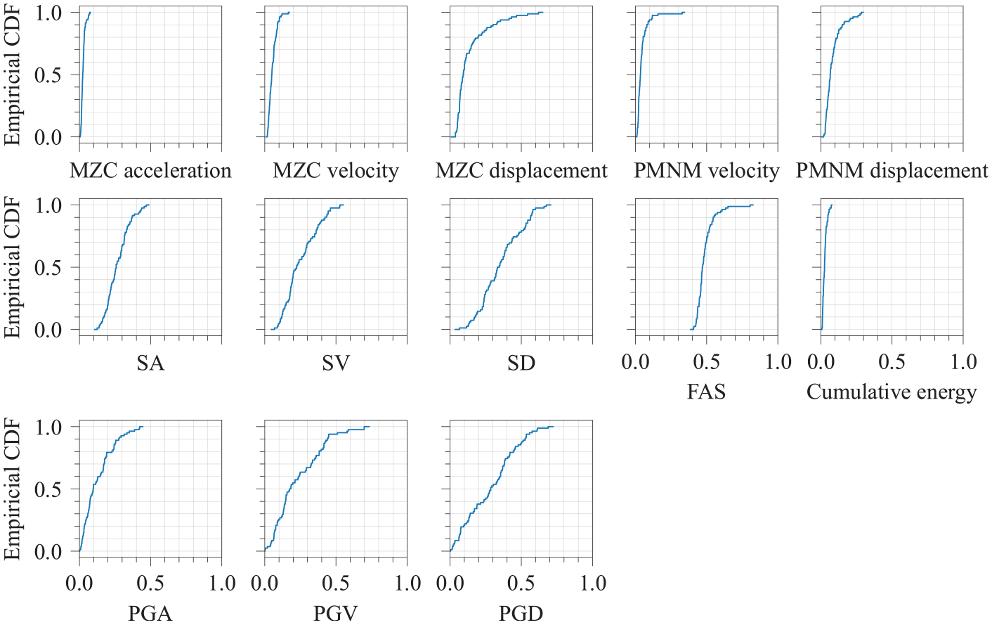
Empirical cumulative distribution (CDF) function of various metrics errors for the Kahramanmaraş, Türkiye, earthquake (Mw = 7.8) dataset.
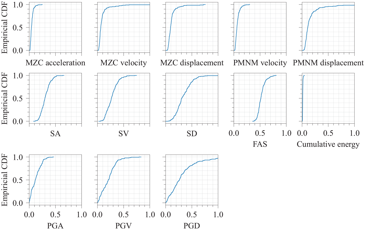
Empirical cumulative distribution (CDF) function of various metrics errors for the NGA-West2 dataset.
Goodness-of-fit score
For further evaluation, the GoF score (Olsen and Mayhew, 2010) is used to quantitatively compare a random simulation with its corresponding target record from the selected datasets. GoF scores are computed for the 13 considered metrics in the previous section. Figure 22 shows the mean GoF scores of the 13 metrics for each component at each station for the Kahramanmaraş earthquake dataset. The GoF scores are consistently above 65, indicating a very good fit for each target record (Olsen and Mayhew, 2010). The consistent GoF scores across different RJB values, as well as for pulse-like and non-pulse-like motions of this event, indicate that the improved model performs efficiently and consistently across the dataset, from near-fault pulse-like to far-field non-pulse-like motions. Figure 23 shows similar consistent performance for the NGA-West2 dataset, indicating that the improved model effectively captures ground motions with notable low-frequency content, typical of pulse-like motions.
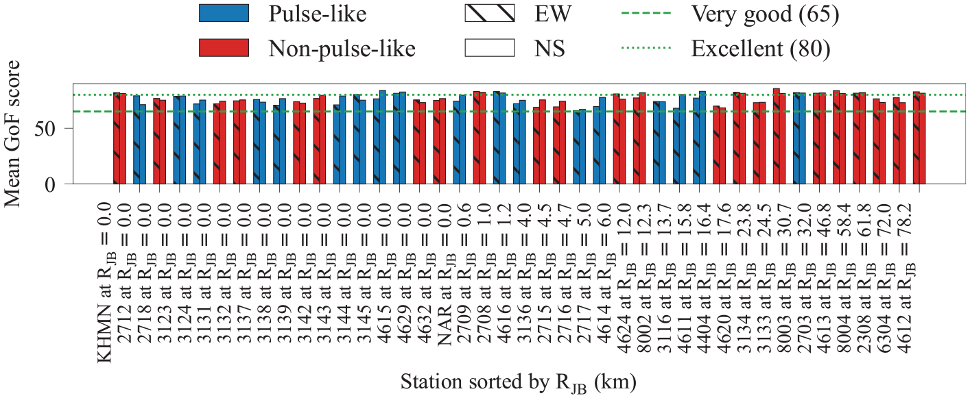
Mean goodness-of-fit (GoF) scores for the east-west (EW) and north-south (NS) components across stations for the Kahramanmaraş, Türkiye, earthquake dataset.
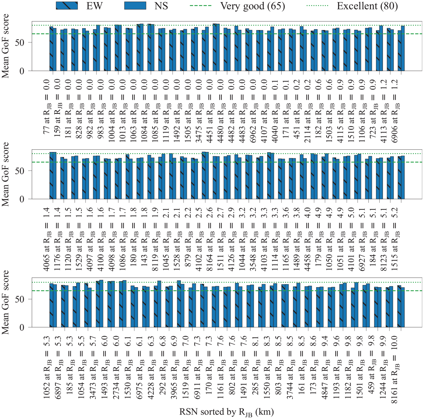
Mean goodness-of-fit (GoF) scores for the east-west (EW) and north-south (NS) components across record sequence number (RSN) for the NGA-West2 dataset.
To evaluate the performance of the improved model for each metric individually, the mean GoF score for each metric is calculated within each dataset. Figures 24 and 25 show the mean GoF scores of each metric, averaged across all stations for the Kahramanmaraş earthquake and pulse-like NGA-West2 datasets, respectively. The results show that the simulations achieve a very good fit for all metrics, except for FAS, which shows a fair fit (GoF > 45), mostly due to the abrupt amplitude variations discussed previously.
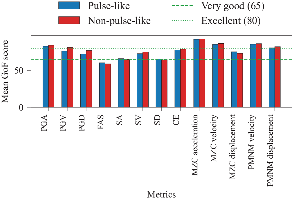
Mean goodness-of-fit (GoF) scores for each metric averaged across all stations, for pulse-like and non-pulse-like motions from the Kahramanmaraş, Türkiye, earthquake dataset.
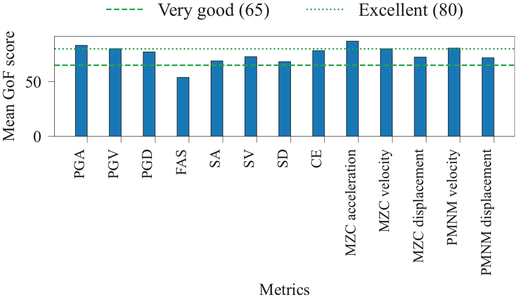
Mean goodness-of-fit (GoF) scores for each metric, averaged across all stations, for pulse-like motions from the NGA-West2 dataset.
Inter-period correlation of spectral acceleration ordinates
Furthermore, the correlations between the spectral acceleration ordinates of the recorded motions and the corresponding simulated motions within periods of 0.04–10 s are compared. These correlations can be an important indicator of the seismic demand in multi-degree-of-freedom (MDoF) systems that are excited at various vibration periods (Burks and Baker, 2014). Figure 26 illustrates these correlations separately for the Kahramanmaraş earthquake and NGA-West2 datasets. It includes recorded motions and individual simulated motions (one random simulation per target record). It is noteworthy that considering a specific set of model parameters corresponding to a station (a recorded motion), a set of simulations in that station does not show a significant correlation due to the stochasticity introduced by underlying white noise. However, when different stations (different sets of parameters) are considered, even with a single random simulation, correlations emerge that align with those observed in real records.
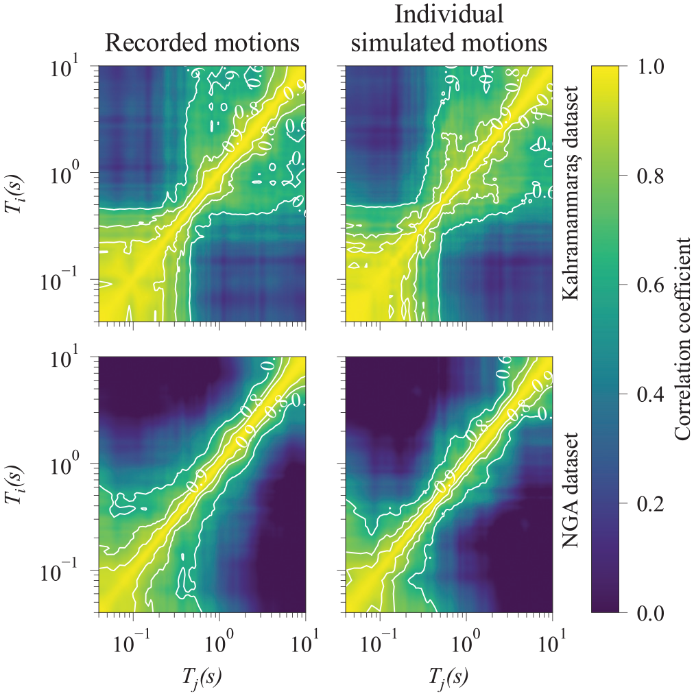
Correlations between spectral acceleration ordinates of recorded and individual simulated motions for the pulse-like and non-pulse-like Kahramanmaraş earthquake dataset (top panel) and pulse-like NGA dataset (bottom panel).
Overall, the simulated and target ground motions exhibit similar evolutionary features. The identified model parameters implicitly consider the properties of the earthquake and site corresponding to a target motion. Thus, the improved model can generate a set of ground motions suitable for designing and evaluating a structure for that specific earthquake and site characteristics.
In future studies, a database of model parameters can be obtained by fitting to many rotated accelerograms with known earthquake and site characteristics. However, further studies are necessary to determine whether these model parameters exhibit a meaningful physical relationship with those characteristics. If such a relationship is established, predictive equations for the model parameters can be developed based on the considered earthquake and site characteristics. The outcome enables the simulation of horizontal orthogonal ground motions for a specified earthquake and site characteristics, using the improved stochastic model following similar procedures in previous studies (Dabaghi and Der Kiureghian, 2018; Rezaeian and Der Kiureghian, 2012; Sgobba et al., 2011).
Conclusion
This study improves the fully non-stationary site-based stochastic ground motion simulation model developed by Rezaeian and Der Kiureghian (2008). The model is improved to have a broader applicability range by representing multiple strong phases in ground motions as well as low-frequency contents which might be due to near-fault directivity effects or potential long-period deep basin effects without adding deterministic velocity pulse model or post-processing filters. An adjustment to the formulation is proposed and is presented in both time and frequency domains. A new modulating function is proposed that can account for the arrival of energy in multiple strong phases. Moreover, a new band-pass filter with additional parameters representing evolutionary bandwidths and dominant frequencies of the ground motion is proposed. This enhancement aims to better represent the lower-frequency content of ground motions, thereby implicitly accounting for the near-fault rupture directivity pulses and potential long-period basin effects. The improved formulation of the model, along with the proposed filter, omits the need for additional post-processing. This consequently eliminates the average bias in the total energy of synthetics and the need for correction factors present in previous site-based stochastic models. On the downside, the additional filter parameters necessitate an adjustment to the objective functions used in parameter identification. However, the simplicity of the model is still preserved through separable temporal and spectral non-stationarities and all parameters can be identified by matching to the time domain CE of the acceleration and the mean zero-level crossings of the acceleration, velocity, and displacement time-series of a target motion.
The proposed simulation model’s performance was evaluated, and the expanded applicability range was tested by simulating the February 6, 2023, Kahramanmaraş (Türkiye) earthquake (Mw = 7.8). The model was further validated for its ability to represent low-frequency content using a near-fault pulse-like dataset from the NGA-West2 database. These datasets represent a diverse set of earthquakes and site characteristics, exhibiting near-fault, far-field, pulse-like, non-pulse-like, single, and multiple strong phase motions. To discuss the model in more detail, four example target accelerograms were selected from the Northridge 1994, Imperial Valley 1979, L’Aquila 2009, and Kahramanmaraş 2023 earthquake events. The validation of the improved stochastic model was performed through both visual and quantitative comparisons. The visual comparisons focused on the four selected records, and quantitative assessments considered both datasets, evaluating various validation metric errors, GoF scores, and inter-period correlations. The results demonstrated an overall good agreement between the simulated and observed motions, with favorable inter-period correlations, and satisfactory errors across the datasets. The GoF scores consistently ranged from very good to excellent for all stations, regardless of ground motion characteristics.
These results indicate that, given the identified parameters for specific earthquake and site characteristics, with the proposed improvements the stochastic model can efficiently simulate a wide range of ground motions, including near-fault pulse-like and multiple strong phase motions, without requiring additional deterministic models and post-processing procedures.
Future research could investigate the potential for scaling model parameters with specific earthquake and site characteristics. In addition, the model’s variability could be explored through comparisons to the standard deviations of empirical ground motion models. However, this requires either a complete set of observed records or the development of a scaling law for model parameters to effectively validate the model’s variability.
Supplemental Material
sj-docx-1-eqs-10.1177_87552930251331981 – Supplemental material for Broadband stochastic simulation of earthquake ground motions with multiple strong phases with an application to the 2023 Kahramanmaraş, Turkey (Türkiye), earthquake
Supplemental material, sj-docx-1-eqs-10.1177_87552930251331981 for Broadband stochastic simulation of earthquake ground motions with multiple strong phases with an application to the 2023 Kahramanmaraş, Turkey (Türkiye), earthquake by SM Sajad Hussaini, Shaghayegh Karimzadeh, Sanaz Rezaeian and Paulo B Lourenço in Earthquake Spectra
Footnotes
Authors’ note
Any use of trade, firm, or product names is for descriptive purposes only and does not imply endorsement by the U.S. Government.
Declaration of conflicting interests
The author(s) declared no potential conflicts of interest with respect to the research, authorship, and/or publication of this article.
Funding
The author(s) disclosed receipt of the following financial support for the research, authorship, and/or publication of this article: This work was partly financed by FCT/MCTES through national funds (PIDDAC) under the R&D Unit Institute for Sustainability and Innovation in Structural Engineering (ISISE), under reference UIDB/04029/2020 (doi.org/10.54499/UIDB/04029/2020), and under the Associate Laboratory Advanced Production and Intelligent Systems (ARISE) under reference LA/P/0112/2020. This study has been partly funded by the STAND4HERITAGE project that has received funding from the European Research Council (ERC) under the European Union’s Horizon 2020 research and innovation program (grant agreement no. 833123), as an Advanced Grant. This work is partly financed by national funds through FCT (Foundation for Science and Technology), under grant agreement UI/BD/153379/2022 attributed to the first author.
Data and resources
The recorded ground motions and their associated information were obtained from the NGA-West2 website accessible at https://ngawest2.berkeley.edu/site and ESM databases website accessible at https://esm-db.eu. A Python package implemented in object-oriented programming, along with the necessary instructions for the proposed improved stochastic ground motion simulation model, is available at: https://github.com/Sajad-Hussaini/sgsim with DOI: ![]() .
.
Supplemental material
Supplemental material for this article is available online.
References
Supplementary Material
Please find the following supplemental material available below.
For Open Access articles published under a Creative Commons License, all supplemental material carries the same license as the article it is associated with.
For non-Open Access articles published, all supplemental material carries a non-exclusive license, and permission requests for re-use of supplemental material or any part of supplemental material shall be sent directly to the copyright owner as specified in the copyright notice associated with the article.