Accounting for ground-motion uncertainty in empirical seismic fragility modeling

Abstract

Seismic fragility models provide a probabilistic relation between ground-motion intensity and damage, making them a crucial component of many regional risk assessments. Estimating such models from damage data gathered after past earthquakes is challenging because of uncertainty in the ground-motion intensity the structures were subjected to. Here, we develop a Bayesian estimation procedure that performs joint inference over ground-motion intensity and fragility model parameters. When applied to simulated damage data, the proposed method can recover the data-generating fragility functions, while the traditionally used method, employing fixed, best-estimate, intensity values, fails to do so. Analyses using synthetic data with known properties show that the traditional method results in flatter fragility functions that overestimate damage probabilities for low-intensity values and underestimate probabilities for large values. Similar trends are observed when comparing both methods on real damage data. The results suggest that neglecting ground-motion uncertainty manifests in apparent dispersion in the estimated fragility functions. This undesirable feature can be mitigated through the proposed Bayesian procedure.

Introduction

Procedures for earthquake risk assessments often rely on probabilistic relations between ground-shaking intensity and physical damage to elements of the built environment. A fragility function plots the probability of reaching or exceeding a certain damage limit state for increasing ground-motion intensity measure ( $\mathrm{IM}$ ) levels. The fragility function parameters are derived from expert opinion (e.g. Hadlos et al., 2023; Rojahn and Sharpe, 1985) or estimated from data that are either generated through structural analyses of building archetypes, the so-called mechanical or analytical approach (e.g. Martins and Silva, 2021; Mosalam et al., 1997), or gathered after an earthquake event, the so-called empirical approach (e.g. Basöz and Kiremidjian, 1998; Rossetto et al., 2014).

Besides challenges in quality and coverage of post-earthquake damage surveys, empirical fragility modeling also requires assumptions on the $\mathrm{IM}$ values that caused the observed damage (Rossetto and Ioannou, 2018). These values are only known at the locations of seismic network stations and are uncertain at other locations. Thus, if a group of damaged buildings is observed, we do not know a-priori whether they were damaged because they were particularly vulnerable or the ground shaking was particularly strong, or because of both. This study aims to provide further insights into this causality dilemma and proposes a new methodology to estimate fragility function parameters.

One common approach to address this causality dilemma assumes fixed, best-estimate, $\mathrm{IM}$ values for parameter estimation (Rossetto et al., 2014). The fixed values represent best estimates that are typically chosen as the median of the $\mathrm{IM}$ distribution conditional on available data from seismic network stations (e.g. from a ShakeMap system). This fixed $\mathrm{IM}$ approach served as the basis for the vast majority of available empirical fragility functions, including early (e.g. Basöz and Kiremidjian, 1998) and recent studies (e.g. Rosti et al., 2021). By considering fixed $\mathrm{IM}$ values, such an approach does not account for potential deviations of the actual $\mathrm{IM}$ from this best estimate. The sensitivity of estimated fragility function parameters with respect to $\mathrm{IM}$ uncertainty was examined in the work by Ioannou et al. (2015) through simulated case studies. They found that unrealistically dense seismic networks are required to recover the “true” fragility parameters used to generate the data. For realistic network configurations, however, the approach based on fixed $\mathrm{IM}$ values led to substantial differences between estimated and “true” parameters. Approaches to account for $\mathrm{IM}$ uncertainty vary in the existing literature. For example, King et al. (2005) focused on damage survey data collected within a limited distance to a seismic network station. Lallemant et al. (2015) suggested weighting the observations according to the inverse of the remaining $\mathrm{IM}$ variance, thus assigning higher weight to data collected close to the stations. Ioannou et al. (2015) simulated numerous $\mathrm{IM}$ values at the survey locations and performed parameter estimation for each simulation run. The resulting set of estimated parameters was then assumed to reflect $\mathrm{IM}$ uncertainty.

While aiming to account for $\mathrm{IM}$ uncertainty, the above approaches miss a crucial component of the causality dilemma, which is best explained by considering the inverse problem, where the true fragility function parameters are available. In this hypothetical case, studied in the work by Pozzi and Wang (2018), the damage observations serve as noisy measurements of the uncertain $\mathrm{IM}$ values. Consequently, these observations can be used to obtain a constrained estimate of the $\mathrm{IM}$ values that caused the damage.

In cases of practical interest, both the fragility parameters and the $\mathrm{IM}$ values are uncertain. This study presents a Bayesian approach to estimate their joint posterior distribution, which can account for uncertainty in both the $\mathrm{IM}$ values and the fragility parameters. We start with an overview of fragility function definitions, followed by mathematical descriptions of the proposed Bayesian parameter estimation approach and the traditional, fixed $\mathrm{IM}$ , approach. Both methods are first explained on a simplified example and then compared using data from the 2009 L’Aquila (Italy) earthquake.

Fragility functions

Empirical fragility modeling aims to estimate the fragility function parameters using observed or estimated values of IMs and building damage states. Damage states are obtained from post-earthquake building inspections, where experts describe the building characteristics and the sustained damage based on pre-specified guidelines and data-recording forms. Information on the building characteristics pertains to the material and the type of the load-resisting system, and geometrical attributes such as the number of stories. Buildings with similar characteristics are grouped into a “building class” with a corresponding set of fragility functions. Damage descriptions are commonly reduced to ordered, collectively exhaustive and mutually exclusive damage states (e.g. no, slight, moderate, heavy, and complete damage), which are numerically encoded as $\mathrm{ds}\in \{0,1,...,c\}$ . To ease the notation in the following definitions, we consider a single building class and assume that all damage observations for buildings of that class are treated equally.

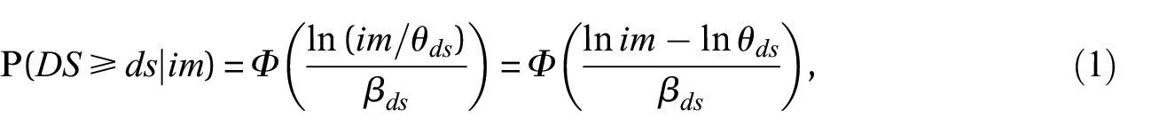
The log-normal cumulative distribution is the most common functional form for fragility functions

$$\mathrm{P}(DS\ge ds|im)=\Phi \left(\frac{\ln (im/{\theta }_{ds})}{{\beta }_{ds}}\right)=\Phi \left(\frac{\ln im-\ln {\theta }_{ds}}{{\beta }_{ds}}\right),$$

(1)

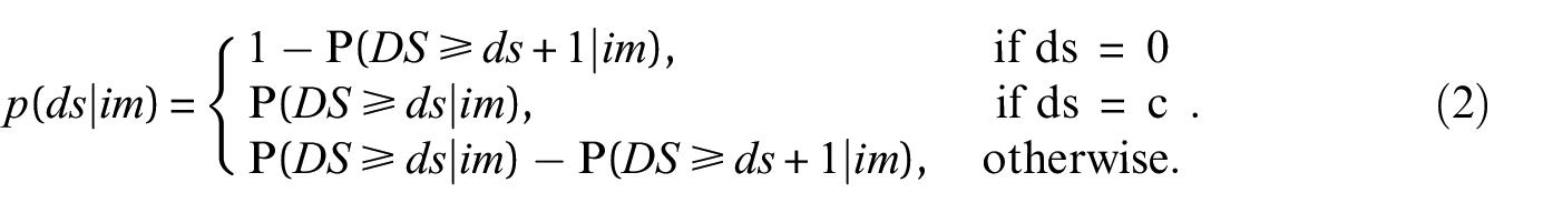
where $\Phi (·)$ is the standard normal cumulative distribution function, ${\theta }_{\mathrm{ds}}$ denotes the median $\mathrm{IM}$ which causes the structure to reach or exceed $\mathrm{ds}$ , and ${\beta }_{\mathrm{ds}}$ is the standard deviation of the $\ln \mathrm{IM}$ , here referred to as the dispersion parameter. From the fragility functions, one obtains the probability mass function, $\mathrm{P}(\mathrm{DS}=\mathrm{ds}|\mathrm{im})=p(\mathrm{ds}|\mathrm{im})$ , as

$$p(ds|im)=\{\begin{array}{cc}1-\mathrm{P}(DS\ge ds+1|im),& \mathrm{if}\mathrm{ds}=\mathrm{0}\\ \mathrm{P}(DS\ge ds|im),& \mathrm{if}\mathrm{ds}=\mathrm{c}\\ \mathrm{P}(DS\ge ds|im)-\mathrm{P}(DS\ge ds+1|im),& \mathrm{otherwise}.\end{array}.$$

(2)

To prevent negative probabilities in Equation 2, we assume an identical dispersion parameter $\beta$ for all damage states. This avoids a crossing of the fragility functions and is a standard assumption taken in analytical and empirical fragility modeling for ordered damage states (e.g. Martins and Silva, 2021; Rosti et al., 2021). For $c+1$ damage states, we thus have $c$ increasing parameters ${\theta }_1<{\theta }_2<\dots <{\theta }_c$ and one common dispersion parameter $\beta$ .

A second fragility function definition, equivalent to Equation 1, is obtained from the cumulative probit model (Lallemant et al., 2015). By introducing the threshold parameters ${\eta }_{\mathrm{ds}}={\beta }^{-1}\ln {\theta }_{\mathrm{ds}}$ , this alternative definition reads as

$$\mathrm{P}(DS\ge ds|im)=\Phi \left({\beta }^{-1}\ln im-{\eta }_{ds}\right).$$

(3)

Following the work by Nguyen and Lallemant (2022), we use the re-parametrized definition of Equation 3 with the transformed parameters ${\eta }_{\mathrm{ds}}$ still being of increasing order. To account for this ordering in the estimation algorithms, we introduce positive parameters ${\delta }_{\mathrm{ds}}={\eta }_{\mathrm{ds}}-{\eta }_{\mathrm{ds}-1}$ for states $\mathrm{ds}>1$ . The parameters of interest are collectively denoted as vector $\mathbf{\vartheta }={[\beta ,{\eta }_1,{\delta }_2,\dots ,{\delta }_c]}^{\mathrm{T}}$ . Finally, we denote the fragility model in terms of the probability mass function $p(\mathrm{ds}|\mathrm{im},\mathbf{\vartheta })$ , where we explicitly condition on parameter vector $\mathbf{\vartheta }$ .

The use of log-normal fragility functions—leading to the cumulative probit model—dates back to earthquake risk assessments of critical infrastructure components (e.g. Kennedy et al., 1980) and is well-established in disaster risk analysis (e.g. Dolce et al., 2021; Kircher et al., 1997) and in performance-based earthquake engineering (e.g. Baker, 2015; Porter et al., 2007). Yet, the herein presented estimation algorithms can also be used for alternative models, such as the cumulative logistic model employed in the work by Basöz and Kiremidjian (1998).

Estimating fragility function parameters

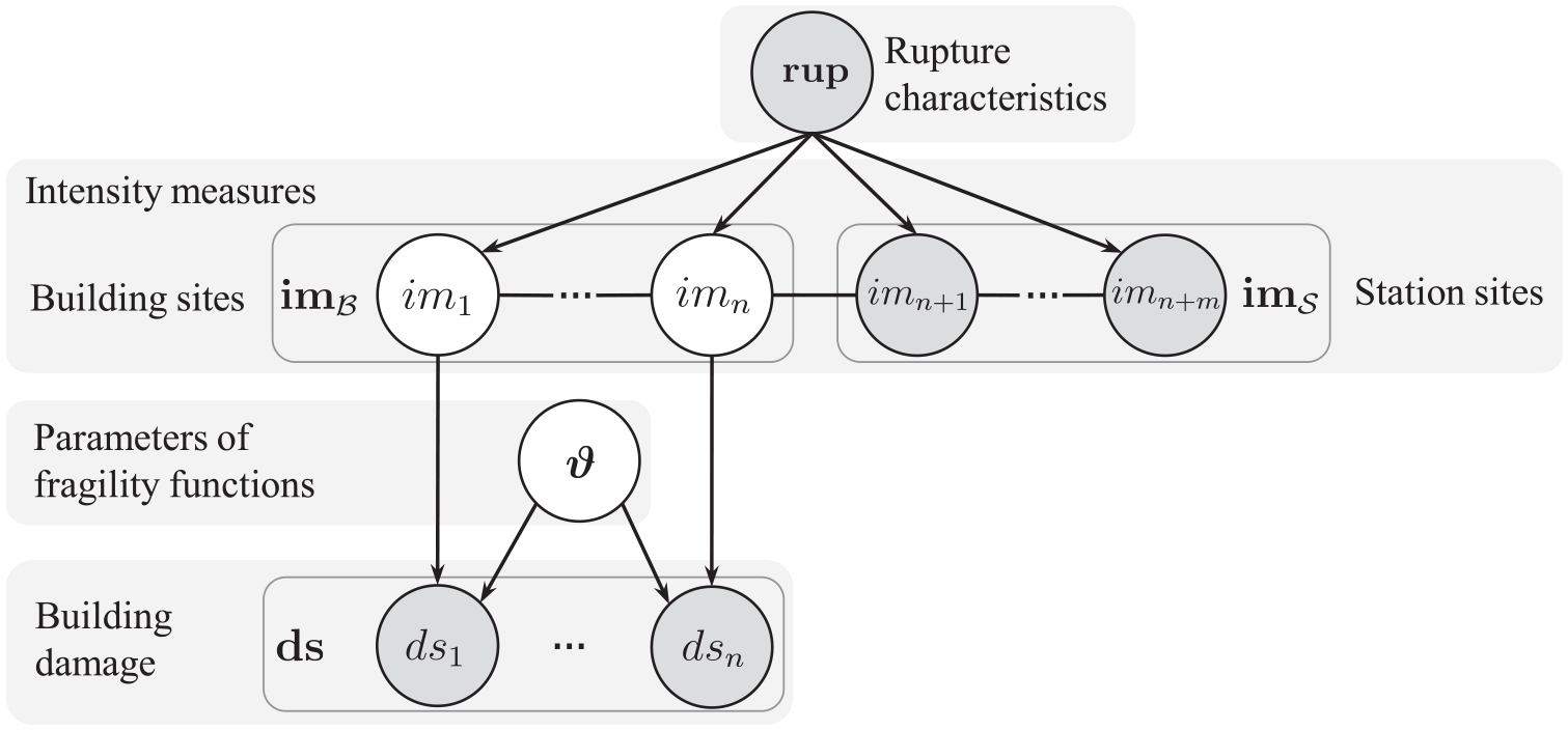
Figure 1 depicts the probabilistic model relating the variables involved in the estimation of $\mathbf{\vartheta }$ by considering a damage dataset from $n$ buildings gathered after an earthquake with rupture characteristics $\mathbf{rup}$ . The fragility model of Equation 2 relates the observed damage states, $\mathbf{ds}=[d{s}_i,\dots ,d{s}_n{]}^{\mathrm{T}}$ , to the IM values at the locations of the surveyed buildings, $\mathbf{i}{\mathbf{m}}_{\mathcal{B}}=[i{m}_1,\dots ,i{m}_n{]}^{\mathrm{T}}$ . Knowing the latter would allow estimating $\mathbf{\vartheta }$ with similar techniques used in analytical fragility modeling (e.g. Baker, 2015). In most cases, however, we only know the $\mathrm{IM}$ values at the locations of seismic stations, here denoted as $\mathbf{i}{\mathbf{m}}_{\mathcal{S}}=[i{m}_{n+1},\dots ,i{m}_{n+m}{]}^{\mathrm{T}}$ for the case of $m$ stations, while their counterparts at the survey locations are uncertain.

Figure 1.

Probabilistic model to estimate fragility function parameters using data from building damage surveys and seismic network stations. Observed and unobserved variables are indicated with gray and white circles, respectively. The arrows indicate directed relationships between the variables. The horizontal lines illustrate that the IMs follow a joint multivariate distribution.

To constrain the above-mentioned uncertainty, we evaluate the distribution of $\mathbf{i}{\mathbf{m}}_{\mathcal{B}}$ conditional on station data $\mathbf{i}{\mathbf{m}}_{\mathcal{S}}$ and rupture characteristics $\mathbf{rup}$ by following the work by Engler et al. (2022), who present the mathematical background for the most recent version of the United States Geological Survey’s ShakeMap system. Conditional on $\mathbf{rup}$ only, the joint distribution of $\mathbf{i}{\mathbf{m}}_{\mathcal{B}}$ and $\mathbf{i}{\mathbf{m}}_{\mathcal{S}}$ is assumed to be multivariate log-normal (Jayaram and Baker, 2008), with parameters derived from empirical ground-motion models (GMMs) and spatial correlation models. Thus, the conditional distribution of interest also follows a multivariate log-normal distribution, that is, $p(\mathbf{i}{\mathbf{m}}_{\mathcal{B}}|\mathbf{i}{\mathbf{m}}_{\mathcal{S}},\mathbf{rup})=\mathcal{L}\mathcal{N}({\mathbf{\mu }}_{\mathcal{B}|\mathcal{S}},{\mathbf{\Sigma }}_{\mathcal{B}\mathcal{B}|\mathcal{S}})$ . The distributional parameters, ${\mathbf{\mu }}_{\mathcal{B}|\mathcal{S}}$ and ${\mathbf{\Sigma }}_{\mathcal{B}\mathcal{B}|\mathcal{S}}$ are computed via Equations 4 and 5 in the work by Engler et al. (2022), also explained in Appendix A of the electronic supplement.

We next present two methodologies to estimate $\mathbf{\vartheta }$ . The first, traditional, method assumes fixed—or deterministic—values for $\mathbf{i}{\mathbf{m}}_{\mathcal{B}}$ . The second, proposed, method, treats both, $\mathbf{\vartheta }$ and $\mathbf{i}{\mathbf{m}}_{\mathcal{B}}$ , as uncertain and follows a Bayesian approach for inference.

Maximum likelihood inference with fixed IM values

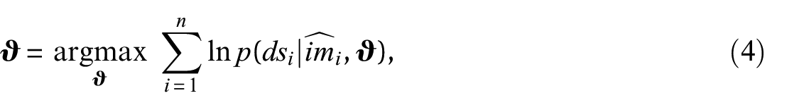
This estimation method replaces uncertain $\mathrm{IM}$ values at the survey sites with fixed, best-estimate, values derived from the conditional distribution $p(\mathbf{i}{\mathbf{m}}_{\mathcal{B}}|\mathbf{i}{\mathbf{m}}_{\mathcal{S}},\mathbf{rup})$ . For site $i$ , the best-estimate value corresponds to ${\widehat{\mathrm{im}}}_i=\exp ([{\mathbf{\mu }}_{\mathcal{B}|\mathcal{S}}{]}_i)$ , which is the median $\mathrm{IM}$ conditional on station data $\mathbf{i}{\mathbf{m}}_{\mathcal{S}}$ . As depicted in Figure 1, the joint distribution of building damage conditional on the $\mathrm{IM}$ values at the building locations factorizes, that is, $p(\mathbf{ds}|\mathbf{i}{\mathbf{m}}_{\mathcal{B}},\mathbf{\vartheta })=\underset{i=1}{\overset{n}{\Pi }}p(d{s}_i|i{m}_i,\mathbf{\vartheta })$ . Assuming fixed $\mathrm{IM}$ values thus offers the advantage that the damage observations of different buildings can be treated independently, which makes it an efficient approach for large amounts of data. The parameters are then estimated by maximizing the log-likelihood

$$\mathbf{\vartheta }=\underset{\vartheta }{\mathrm{argmax}}\sum _{i=1}^n\ln p(d{s}_i|{\widehat{\mathrm{im}}}_i,\mathbf{\vartheta }),$$

(4)

such that the obtained parameter estimates maximize the probability of observing the surveyed damage under the chosen best-estimate $\mathrm{IM}$ values. In the following, we refer to this estimation method as the fixed $\mathrm{IM}$ approach.

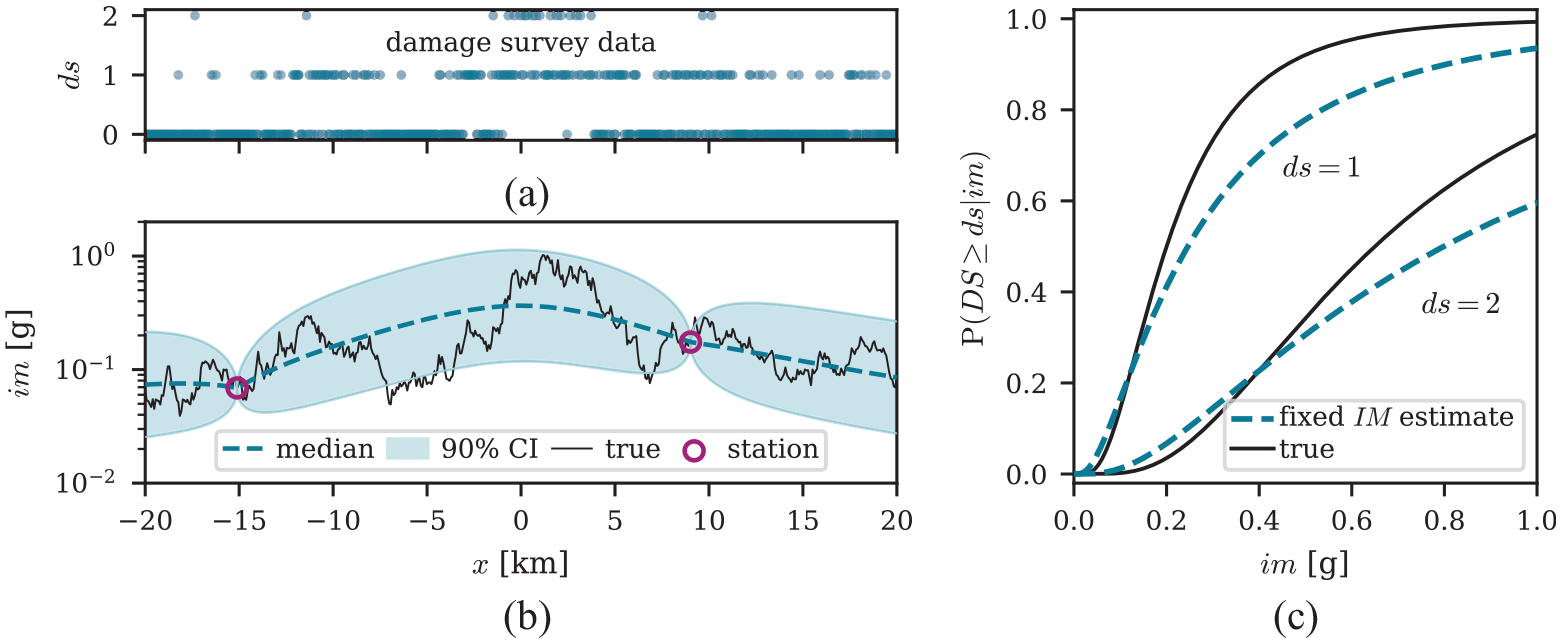
Figure 2 illustrates a one-dimensional example with simulated $\mathrm{IM}$ observations and damage data from two stations and 500 buildings resulting from a magnitude 6 earthquake with an epicenter at $x=0$ km. The assumed fragility parameter values are 0.65, 0.2, and 0.65 g for $\beta$ , ${\theta }_1$ , and ${\theta }_2$ , respectively, and the estimated values are 0.92, 0.25, and 0.80 g. From Figure 2b, we observe the substantial uncertainty around the median of $p(\mathbf{i}{\mathbf{m}}_{\mathcal{B}}|\mathbf{i}{\mathbf{m}}_{\mathcal{S}},\mathbf{rup})$ . By considering fixed $\mathrm{IM}$ values, this approach does not account for deviations of the “true” $\mathrm{IM}$ from this best estimate. The estimated fragility functions, shown in Figure 2c, are flatter than the “true” functions used to generate the data. Such behavior was also observed in the simulated case studies in the work by Ioannou et al. (2015) mentioned in the “Introduction”, and results from an overestimation of the dispersion parameter $\beta$ . This overestimation indicates that $\mathrm{IM}$ uncertainty manifests as apparent uncertainty—or dispersion—in the fragility functions.

Figure 2.

Fragility results from a one-dimensional example with simulated damage survey data. (a) Building damage states plotted versus their location. Damage states are simulated using the assumed “true” fragilities and $\mathrm{IM}$ values. (b) Simulated “true” $\mathrm{IM}$ values, with circles denoting the locations and $\mathrm{IM}$ values for two recording stations. The dashed line indicates the predicted median $\mathrm{IM}$ values and the shaded interval indicates the 90% credibility interval (CI) of the distribution conditional on data from the two stations. (c) The “true” fragility functions and the ones estimated with the fixed $\mathrm{IM}$ approach.

Bayesian inference with uncertain IM values

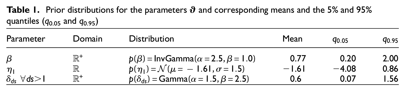
To account for ground-motion uncertainty, we take a Bayesian approach treating both the fragility function parameters, $\mathbf{\vartheta }$ , and the $\mathrm{IM}$ values at the survey sites, $\mathbf{i}{\mathbf{m}}_{\mathcal{B}}$ , as realizations of random variables. The model shown in Figure 1 serves as the prior generative model which gives rise to the observed data. Based on this model, we express the joint posterior distribution of $\mathbf{i}{\mathbf{m}}_{\mathcal{B}}$ and $\mathbf{\vartheta }$ conditional on the triplet of damage survey data, $\mathbf{ds}$ , station data, $\mathbf{i}{\mathbf{m}}_{\mathcal{S}}$ , and rupture characteristics, $\mathbf{rup}$ , as

$$p(\mathbf{\vartheta },\mathbf{i}{\mathbf{m}}_{\mathcal{B}}|\mathbf{ds},\mathbf{i}{\mathbf{m}}_{\mathcal{S}},\mathbf{rup})=(\underset{i=1}{\overset{n}{\Pi }}p(d{s}_i|i{m}_i,\mathbf{\vartheta }))\frac{p(\mathbf{i}{\mathbf{m}}_{\mathcal{B}}|\mathbf{i}{\mathbf{m}}_{\mathcal{S}},\mathbf{rup})p(\mathbf{\vartheta })}{p(\mathbf{ds}|\mathbf{i}{\mathbf{m}}_{\mathcal{S}},\mathbf{rup})},$$

(5)

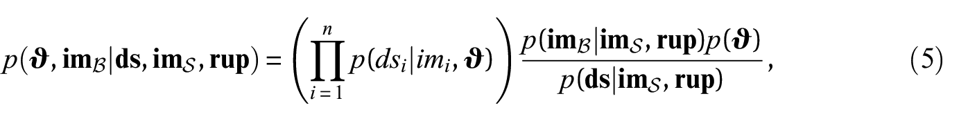
where the denominator, $p(\mathbf{ds}|\mathbf{i}{\mathbf{m}}_{\mathcal{S}},\mathbf{rup})$ , is the marginal likelihood, that is, the probability that the prior model assigns to the observed damage data conditional on station data and rupture characteristics, and $p(\mathbf{\vartheta })$ is the prior distribution of the fragility function parameters. For each parameter, we assign weakly informative priors, stated in Table 1, and assume that the parameters are a-priori independent. These distributions are chosen such that the resulting fragility functions provide sufficient adaptability to cover building classes with varying susceptibility to earthquake damage, as illustrated in Appendix B of the electronic supplement.

Table 1.

Prior distributions for the parameters $\mathbf{\vartheta }$ and corresponding means and the 5% and 95% quantiles (q_0.05 and q_0.95)

Parameter	Domain	Distribution	Mean	$q_{0.05}$	$q_{0.95}$
$\beta$	${\mathbb{R}}^{+}$	$p(\beta )=\mathrm{InvGamma}(\alpha =2.5,\beta =1.0)$	0.77	0.20	2.00
${\eta }_1$	$\mathbb{R}$	$p({\eta }_1)=\mathcal{N}(\mu =-1.61,\sigma =1.5)$	−1.61	−4.08	0.86
${\delta }_{\mathrm{ds}}$ $\forall \mathrm{ds}>1$	${\mathbb{R}}^{+}$	$p({\delta }_{\mathrm{ds}})=\mathrm{Gamma}(\alpha =1.5,\beta =2.5)$	0.6	0.07	1.56

The posterior distribution in Equation 5 is not analytically tractable, thus we use Markov Chain Monte Carlo (MCMC) sampling for Bayesian inference. MCMC is a computational technique used to approximate complex probability distributions. It combines principles from MCMC methods to efficiently sample from a target distribution when direct sampling is not feasible. This makes it particularly valuable for Bayesian statistics, where we aim to draw samples from a certain target posterior. Here, we employ the No-U-Turn Sampler (Hoffman and Gelman, 2014) as implemented in the software library NumPyro (Phan et al., 2019). We obtain 3000 sample sets $(\mathbf{\vartheta },\mathbf{i}{\mathbf{m}}_{\mathcal{B}})$ from the full posterior distribution through four independent MCMC chains with 1000 warm-up steps each. We sometimes report results using central statistics (e.g. mean or median) and credibility intervals (CIs) computed from the posterior samples. The convergence of the MCMC chains is tested by following the recommendations of the work by Vehtari et al. (2021) summarized in Appendix C of the electronic supplement. The implementation details can be found in the provided code repository. ¹

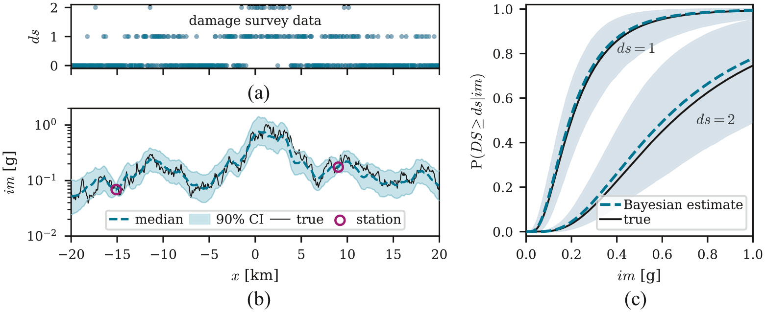
Figure 3 illustrates the posterior samples of $(\mathbf{\vartheta },\mathbf{i}{\mathbf{m}}_{\mathcal{B}})$ , obtained from MCMC, for the same one-dimensional example used in Figure 2. From Figure 3b, we observe how the consideration of the damage survey data allows for an improved estimate on $\mathbf{i}{\mathbf{m}}_{\mathcal{B}}$ compared to the case in Figure 2b that uses solely the available station data. Figure 3c plots the fragility functions obtained from the mean of the sampled parameters (dashed lines, corresponding to 0.65, 0.19, and 0.61 g for $\beta$ , ${\theta }_1$ , and ${\theta }_2$ , respectively), which closely match the “true” data-generating functions. The shaded areas indicate the 90% CI. The latter is the difference between the 95% and 5% quantiles obtained at each im level for all functions computed from the posterior parameter samples. The limited amount of data considered in this simplified example results in relatively large CIs, especially for $\mathrm{ds}=2$ .

Figure 3.

Fragility results from the Bayesian approach for the example from Figure 2: (a) simulated building damage states plotted versus their location. (b) Simulated “true” $\mathrm{IM}$ values, with circles denoting the locations and $\mathrm{IM}$ values for two recording stations. The dashed line and the shaded area indicate the median and the 90% CI of the posterior $\mathrm{IM}$ distribution conditional on station and damage data. (c) The “true” and the estimated fragility functions. The dashed lines show the functions obtained from the mean posterior parameters, and the shaded area indicates the 90% CI.

Accounting for different building characteristics

So far, we have assumed identical fragility functions for all considered buildings. To reflect the heterogeneity in realistic building stocks, the model should account for the differences in structural types, geometry, and other building characteristics. For this purpose, most current regional earthquake risk models use multiple fragility models, each defined for a specific combination of building characteristics. These combinations are here referred to as building classes and denoted with variable $\mathrm{bc}\in \mathcal{B}\mathcal{C}$ , where $\mathcal{B}\mathcal{C}$ is the set of all considered building classes.

The fragility functions for different $\mathrm{bc}$ are commonly assumed to be of the same functional form, that is, the model specified in Equation 3, but with differing parameters. Thus, the total set of parameters is $\mathbf{\vartheta }=\{{\mathbf{\vartheta }}_{\mathrm{bc}}|\mathrm{bc}\in \mathcal{B}\mathcal{C}\}$ . When using the fixed $\mathrm{IM}$ approach, the parameters ${\mathbf{\vartheta }}_{\mathrm{bc}}$ are estimated independently for each $\mathrm{bc}$ . Thus, it may be necessary to use fewer building classes such that a sufficiently large number of observations per class is available. The proposed Bayesian approach jointly estimates the posterior of $\mathrm{IM}$ values and all parameters $\mathbf{\vartheta }$ . This results in a more complex estimation step, but has the advantage that even classes with few observations profit from the reduced uncertainty in the $\mathrm{IM}$ posterior obtained from all observations.

Information on building characteristics is gathered during the building inspection for post-earthquake damage assessment. The herein presented case study makes use of existing studies that defined a set of building classes, $\mathcal{B}\mathcal{C}$ . In the general case, however, the choice of $\mathcal{B}\mathcal{C}$ and the fragility modeling are inherently connected. It often requires an iterative procedure to check which $\mathcal{B}\mathcal{C}$ performs best in distinguishing susceptibility of a building to earthquake damage, while still providing enough observations per building class.

Case study: the 2009 L’Aquila (Italy) earthquake

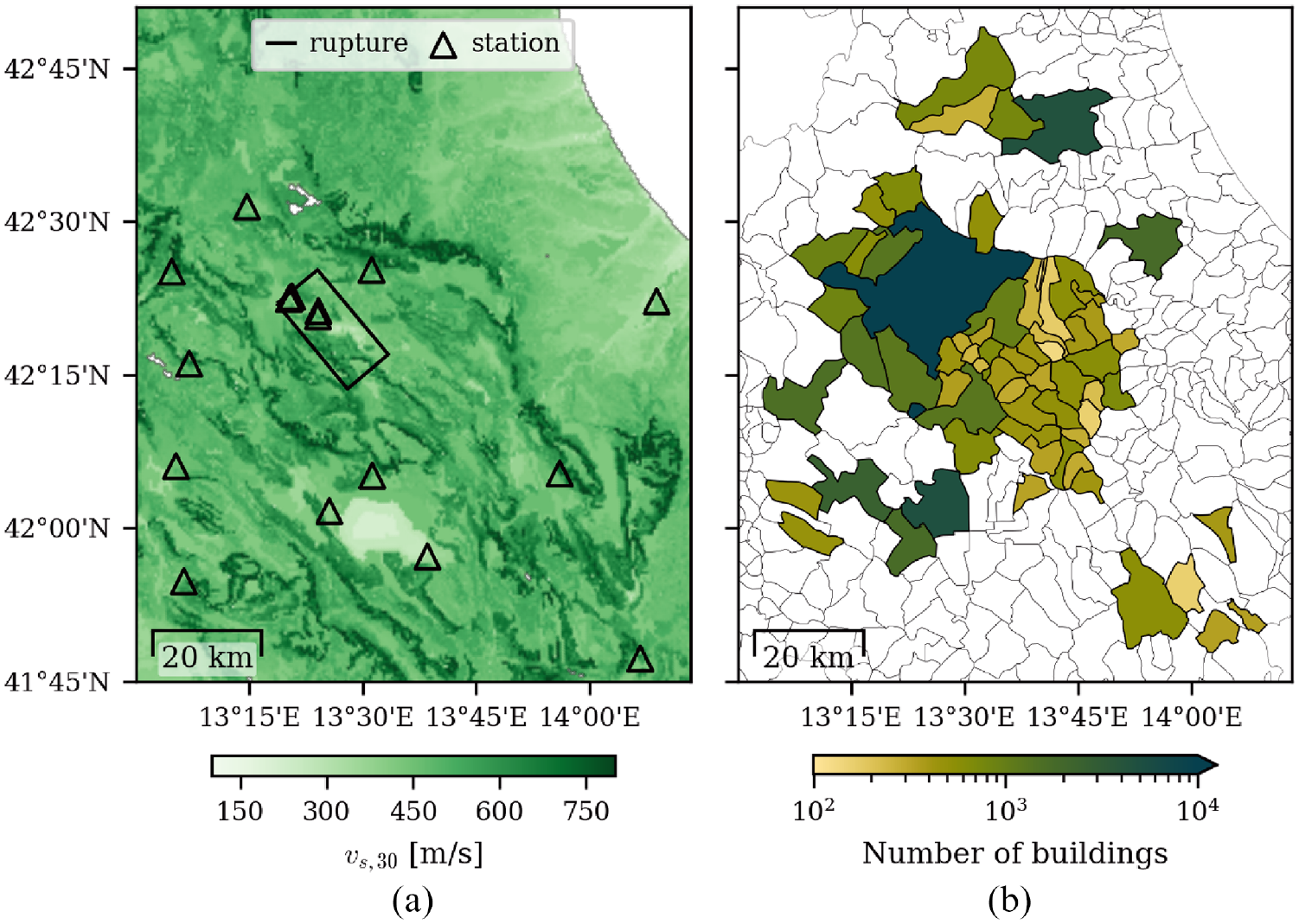
This case study estimates fragility function parameters using data from the 2009 M6 L’Aquila earthquake. The objectives are twofold: first, to apply the proposed Bayesian estimation method on a real dataset and second, to examine the role of $\mathrm{IM}$ uncertainty by comparing the Bayesian estimation results to results from the traditional, fixed $\mathrm{IM}$ approach. The dataset contains results of visual post-earthquake inspections of residential buildings and was published by the Italian Civil Protection Department (Dolce et al., 2019). As such, it provides information on the sustained damage and descriptions of the building characteristics (e.g. the geometry and the structural type). These survey data are combined with rupture characteristics and data from 64 seismic network stations obtained from the Engineering Strong-Motion Database (Luzi et al., 2020). Figure 4a shows the surface projection of the rupture and the stations located within the region of interest together with soil conditions in terms of the 30-m time-averaged shear-wave velocity, $v_{s30}$ , obtained from the work by Mori et al. (2020).

Figure 4.

Overview of the L’Aquila case study region: (a) seismic network stations, projected rupture surface, and soil conditions as measured via $v_{s,30}$ ; (b) number of buildings per municipality in the considered dataset.

The considered dataset consists of 56,400 masonry buildings distributed over 62 municipalities, as shown in Figure 4b. The damage states are derived from the raw inspection results based on Table 1 in the work by Rosti et al. (2021) and consist of six categories: no $(\mathrm{ds}=0)$ , negligible to slight $(\mathrm{ds}=1)$ , moderate $(\mathrm{ds}=2)$ , severe $(\mathrm{ds}=3)$ , very heavy damage, $(\mathrm{ds}=4)$ , and collapse $(\mathrm{ds}=5)$ . In accordance with the national Italian risk assessment (Dolce et al., 2021), we categorize the masonry buildings into three structural types, A, B, and C1, with decreasing susceptibility to earthquake-induced damage. The link between specific attributes in the damage survey and the three structural types are described in Table 10 in the work by Dolce et al. (2019). Finally, fragility parameters are estimated for six building classes, derived from the structural type and the number of stories. Specifically, each type is further divided into low-rise structures (one and two stories) and mid-/high-rise structures (more than two stories), denoted as L and MH, respectively. We estimate six parameters for each building class, leading to a total of 36 parameters.

The above-described dataset was obtained after several pre-processing steps of the raw post-earthquake survey results. One often-encountered challenge in empirical fragility modeling is the under-representation of undamaged buildings. This occurs because inspections may focus preferentially on damaged buildings. To alleviate this issue, we broadly follow the approach taken in the work by Rosti et al. (2021). For each municipality, the number of buildings in the database is compared to statistics from the 2001 National Census (ISTAT, 2001). Municipalities where the available dataset covers at least 90% of the number of buildings indicated in the census statistics are considered as completely surveyed. For municipalities where this ratio is less than 10%, it is assumed that only damaged buildings were inspected, and the remaining buildings are added to the inspection dataset assuming that they are undamaged. Municipalities without any inspection results are not considered. Due to the challenge of inferring the condition of non-inspected buildings, we also omit results from municipalities with ratios between 10% and 90%.

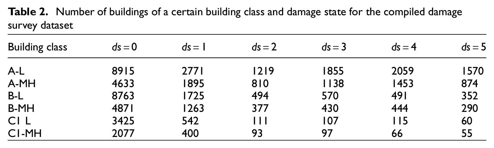
Missing fields in the original inspection dataset and the added undamaged buildings result in some buildings having unknown spatial coordinates, number of stories, or structural type. Buildings with identical or missing coordinates (e.g. the added buildings) are re-distributed based on residential land-use information retrieved from the European settlement map (Corbane and Sabo, 2019). Missing entries on story number and structural type are imputed based on census and survey data. The estimation of a final set of fragility functions for seismic risk analyses would require additional sensitivity studies with respect to these data pre-processing steps including an extensive documentation and collaboration with local experts and governmental agencies on their methods to assess building damage, considering the entire building and its components. Such efforts are required regardless of the employed approach for fragility function estimation and are not within the scope of this illustrative case study. Of the 56,400 masonry buildings in the final dataset, 35,700 (63%) stem from the post-earthquake inspection dataset and 20,700 (27%) undamaged buildings are added based on census data. For each considered building class, Table 2 shows the number of buildings per damage state.

Table 2.

Number of buildings of a certain building class and damage state for the compiled damage survey dataset

Building class	$\mathrm{ds}=0$	$\mathrm{ds}=1$	$\mathrm{ds}=2$	$\mathrm{ds}=3$	$\mathrm{ds}=4$	$\mathrm{ds}=5$
A-L	8915	2771	1219	1855	2059	1570
A-MH	4633	1895	810	1138	1453	874
B-L	8763	1725	494	570	491	352
B-MH	4871	1263	377	430	444	290
C1 L	3425	542	111	107	115	60
C1-MH	2077	400	93	97	66	55

The pre-processed damage dataset, summarized in Table 2, is then used to estimate fragility functions using two approaches: the fixed $\mathrm{IM}$ approach and the proposed Bayesian, MCMC-based, approach. The latter uses the entire conditional distribution $p(\mathbf{i}{\mathbf{m}}_{\mathcal{B}}|\mathbf{i}{\mathbf{m}}_{\mathcal{S}},\mathbf{rup})$ , which requires the storage of the $(n\times n)$ -dimensional matrix ${\mathbf{\Sigma }}_{\mathcal{B}\mathcal{B}|\mathcal{S}}$ . Due to this high memory demand, the size of the considered dataset has to be limited. The inference is run on an NVIDIA V100 tensor core GPU with 25 GB of RAM that allows the consideration of data from n = 14,000 buildings, corresponding to one-fourth of the dataset. The data subset is developed by randomly sampling 25% of the buildings from each building class/damage state combination shown in Table 2. For the computationally less expensive fixed $\mathrm{IM}$ approach, we use the entire dataset.

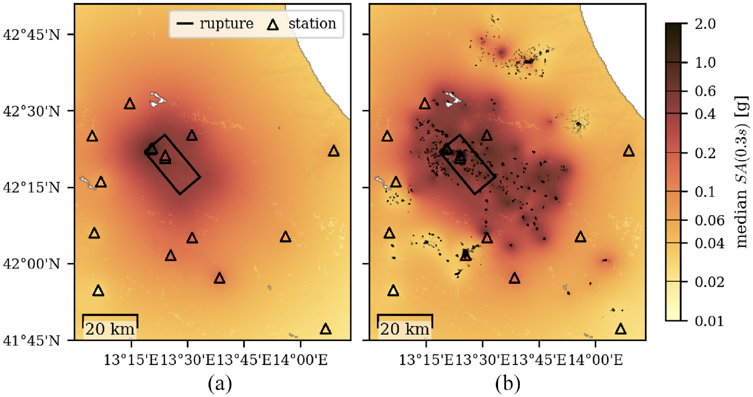
We first estimate fragility functions using $\mathrm{SA}(0.3s)$ as the $\mathrm{IM}$ . Thus, the vectors $\mathbf{i}{\mathbf{m}}_{\mathcal{B}}$ and $\mathbf{i}{\mathbf{m}}_{\mathcal{S}}$ are spectral accelerations at sites of surveyed buildings and network stations, respectively. To compute the conditional distribution $p(\mathbf{i}{\mathbf{m}}_{\mathcal{B}}|\mathbf{i}{\mathbf{m}}_{\mathcal{S}},\mathbf{rup})$ , we use the OpenQuake (Silva et al., 2014) implementation of the Bindi et al.’s (2011) GMM and the spatial correlation model of Esposito and Iervolino (2012). Figure 5a plots the median spectral accelerations conditional on station data $\mathbf{i}{\mathbf{m}}_{\mathcal{S}}$ . Recall that this median value is used to estimate parameters $\mathbf{\vartheta }$ with the fixed $\mathrm{IM}$ approach. The Bayesian approach, however, provides samples from the joint posterior of $\mathbf{i}{\mathbf{m}}_{\mathcal{B}}$ and $\mathbf{\vartheta }$ . The median of the posterior $\mathbf{i}{\mathbf{m}}_{\mathcal{B}}$ samples is plotted in Figure 5b, where the locations of the considered buildings are also indicated. We observe that the resulting spatial $\mathrm{IM}$ pattern is more refined compared to the original map in panel a.

Figure 5.

(a) The spatial distribution of median $\mathrm{SA}(0.3s)$ values conditional on seismic network recordings and (b) additionally conditioned on damage survey data via the proposed Bayesian approach. Network stations and locations of surveyed buildings are indicated with triangles and points, respectively.

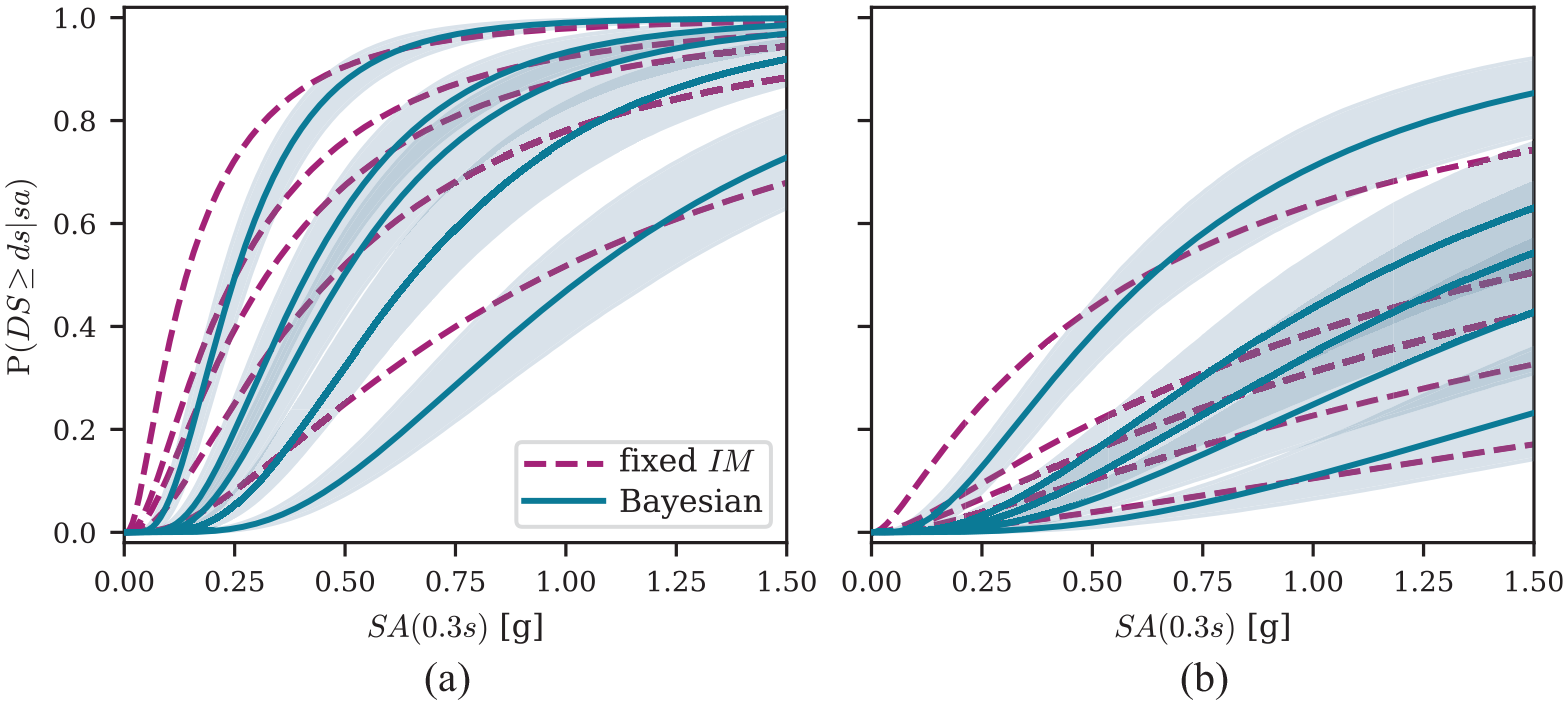
Figure 6 plots the fragility functions of two building classes, A-MH and C1-L, as obtained with the fixed $\mathrm{IM}$ approach and the proposed Bayesian approach. Similar to the one-dimensional example in Figure 2, we observe that the fixed $\mathrm{IM}$ -based parameter estimates lead to flatter fragility functions compared to those obtained from the Bayesian approach, providing higher damage probabilities for low $\mathrm{IM}$ values and lower probabilities for large $\mathrm{IM}$ values. For example, considering building class A-MH in Figure 6a, and a spectral acceleration $\mathrm{SA}(0.3s)=0.25g$ , the fragility functions obtained from the fixed $\mathrm{IM}$ approach predict a 30% probability of reaching or exceeding $\mathrm{ds}=4$ , while this probability decreases to 5% if the mean of the posterior samples is used. For the Bayesian approach, we also note the decrease in the 90% CI compared to the one-dimensional example in Figure 3. This is due to the larger size of the considered damage survey dataset, combined with a larger number of seismic stations.

Figure 6.

Fragility functions for building class (a) A-MH and (b) C1-L estimated from the damage survey data using the fixed $\mathrm{IM}$ and the Bayesian approaches. The five functions correspond to $\mathrm{ds}\in \{1,2,\dots ,5\}$ from the top left to the bottom right. Functions from the Bayesian approach are illustrated using the mean posterior samples (solid lines) and the 90% CI (shaded area).

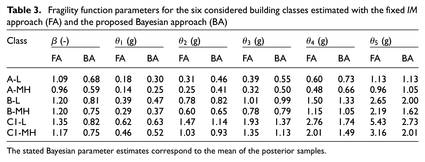
Table 3 provides the estimated fragility function parameters for the six considered building classes. The fixed $\mathrm{IM}$ approach leads to substantially larger estimates of the dispersion parameter $\beta$ , explaining the flatter fragility functions in Figure 6. By fixing $\mathrm{IM}$ values to the best-estimate values plotted in Figure 5a, the variability of the actual, unobserved, $\mathrm{IM}$ values around these best-estimates manifests in apparent dispersion in the estimated fragility functions, as reflected by the large $\beta$ values. Both estimation approaches capture the increasing damage susceptibility expected from the employed building categorization scheme, that is, buildings of type A having lower ${\theta }_{\mathrm{ds}}$ values and thus being more fragile than buildings of type C1. Furthermore, low-rise buildings (e.g. A-L) tend to be less fragile than their counterparts with more than two stories (e.g. A-MH).

Table 3.

Fragility function parameters for the six considered building classes estimated with the fixed $\mathrm{IM}$ approach (FA) and the proposed Bayesian approach (BA)

Class	$\beta$ (-)		${\theta }_1$ (g)		${\theta }_2$ (g)		${\theta }_3$ (g)		${\theta }_4$ (g)		${\theta }_5$ (g)
	FA	BA	FA	BA	FA	BA	FA	BA	FA	BA	FA	BA
A-L	1.09	0.68	0.18	0.30	0.31	0.46	0.39	0.55	0.60	0.73	1.13	1.13
A-MH	0.96	0.59	0.14	0.25	0.25	0.41	0.32	0.50	0.48	0.66	0.96	1.05
B-L	1.20	0.81	0.39	0.47	0.78	0.82	1.01	0.99	1.50	1.33	2.65	2.00
B-MH	1.20	0.75	0.29	0.37	0.60	0.65	0.78	0.79	1.15	1.05	2.19	1.62
C1-L	1.35	0.82	0.62	0.63	1.47	1.14	1.93	1.37	2.76	1.74	5.43	2.73
C1-MH	1.17	0.75	0.46	0.52	1.03	0.93	1.35	1.13	2.01	1.49	3.16	2.01

The stated Bayesian parameter estimates correspond to the mean of the posterior samples.

Results using alternate IMs

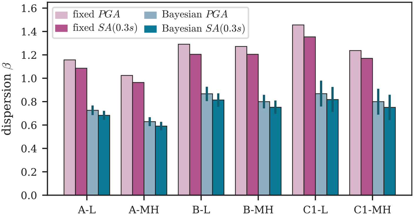
Only few empirical fragility functions are derived for spectral accelerations, while the majority are based on $\mathrm{PGA}$ (e.g. Rosti et al., 2021). The use of $\mathrm{SA}(0.3s)$ above was motivated by its use in analytical fragility modeling where it is often seen as a more efficient predictor of building response (e.g. Romão et al., 2021). Given this assumption, we would expect smaller dispersion values, $\beta$ , when using spectral accelerations. Figure 7 shows the $\beta$ values estimated for both $\mathrm{IM}$ s using the fixed $\mathrm{IM}$ and the Bayesian approaches. Indeed, the $\beta$ values for $\mathrm{SA}(0.3s)$ are slightly smaller for both approaches. The small difference may be explained by the fact that we focus on masonry buildings that are almost all less than four stories tall, thus representing relatively heavy and non-ductile structures for which $\mathrm{PGA}$ can be an adequate fragility predictor. For the remainder of this study, we continue with $\mathrm{SA}(0.3s)$ as the IM of interest.

Figure 7.

Comparison of estimated $\beta$ values from the fixed $\mathrm{IM}$ and the Bayesian approach for $\mathrm{PGA}$ and $\mathrm{SA}(0.3s)$ .

Comparison for different GMMs

So far, we used the Bindi et al.’s (2011) GMM and the Esposito and Iervolino’s (2012) correlation model to establish the distribution of $\mathrm{IM}$ values conditional on station data (illustrated by its median in Figure 5a). These models are both calibrated on Italian ground-motion data, and we denote this combination as GMM1. Here, we will compare the parameter estimates obtained with GMM1 to the ones resulting from a second combination, named GMM2, that uses the Chiou and Youngs’ (2014) GMM and the correlation model of Bodenmann et al. (2023). Both GMM2 models are estimated on the same global ground motion dataset. The change of input motion models affects only the $\mathbf{i}{\mathbf{m}}_{\mathcal{B}}$ distribution in Figure 1, and we use the alternate distribution to then re-estimate the fragility parameters, $\mathbf{\vartheta }$ .

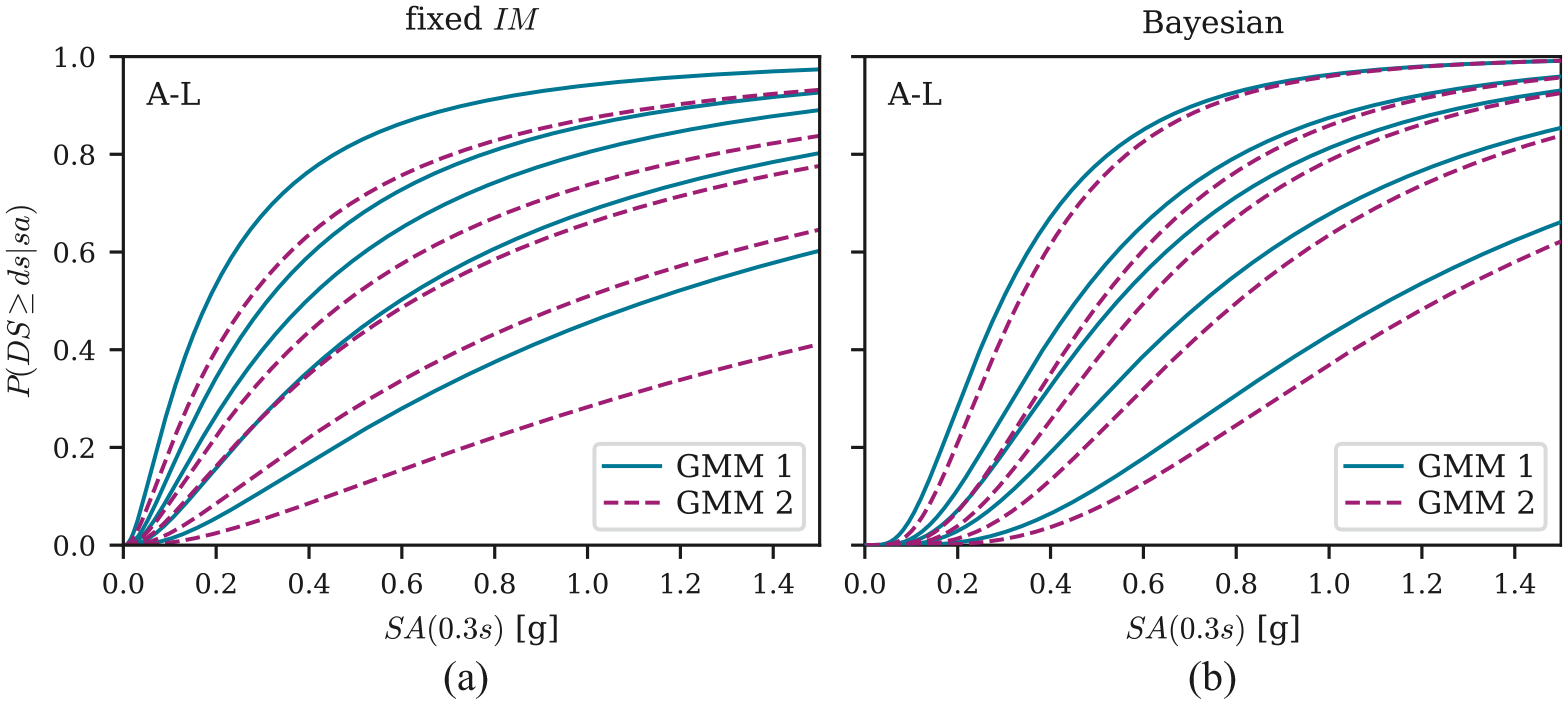
Figure 8 shows the fragility functions for A-L buildings derived using GMM1 and GMM2, respectively. For better readability, only the mean Bayesian estimates are shown. From Figure 8b, we observe that the functions obtained from the Bayesian approach are similar for both GMMs, while Figure 8a indicates a substantial sensitivity on the underlying GMM for the fixed $\mathrm{IM}$ approach. In the latter case, the parameter estimates based on GMM2 indicate less fragile buildings. The reasons for these differences are explained below.

Figure 8.

Comparison of fragility functions for building class A-L that are estimated using two different combinations of ground motion and spatial correlation models (GMM1 and GMM2) through the (a) fixed $\mathrm{IM}$ approach and (b) the proposed Bayesian approach.

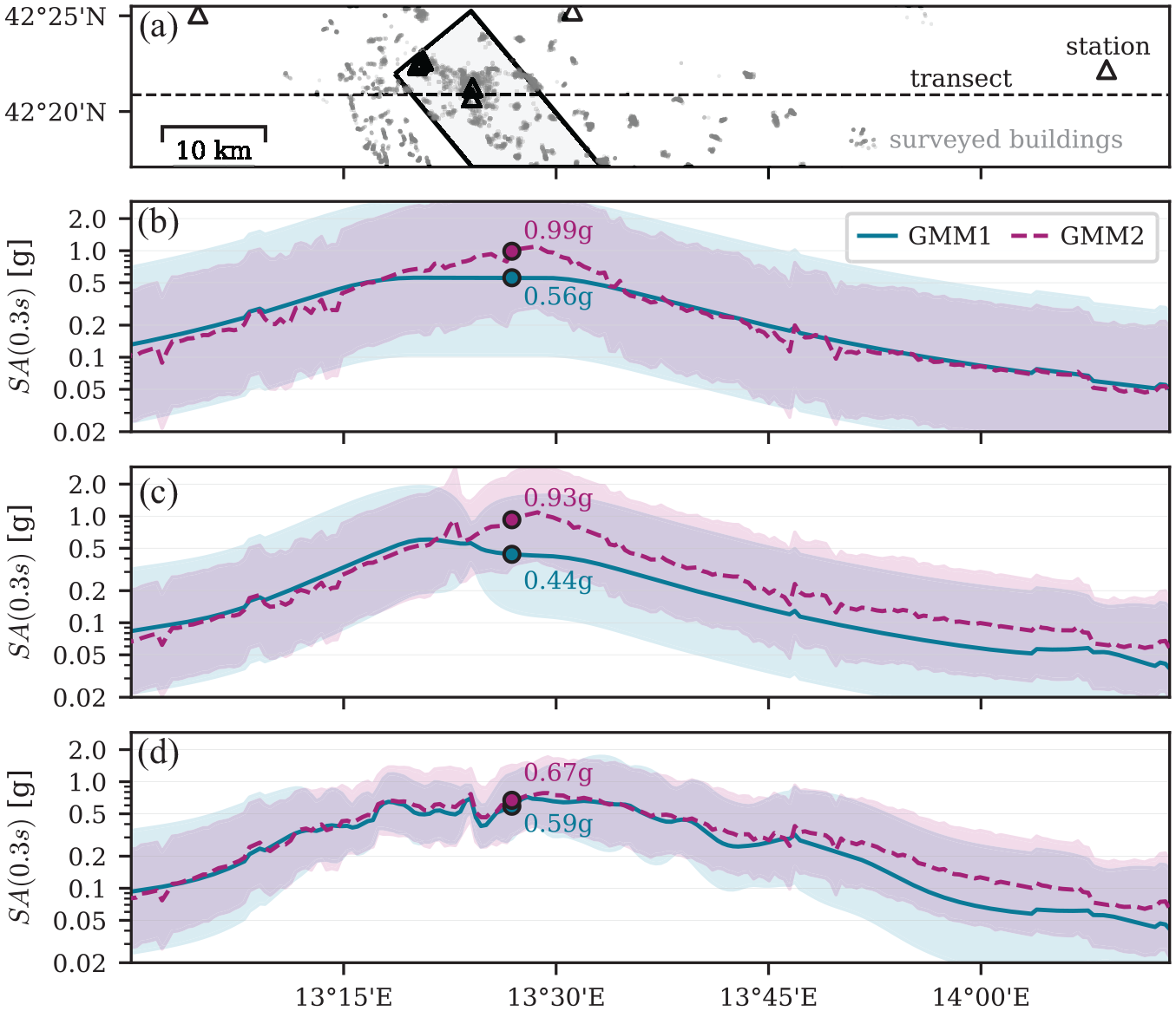
The alternate models within GMM1 and GMM2 predict differing $\mathrm{SA}(0.3s)$ values for the rupture due to differences in functional forms, dependent variables, and the data used in fitting the models’ parameters. To illustrate these differences, we compare the $\mathrm{SA}(0.3s)$ predictions along the horizontal transect illustrated in Figure 9a. Figure 9b plots the predictive distributions in terms of the median and the 90% CI, prior to taking into account station recordings and damage survey data. For sites located within the rupture surface projection, GMM2 predicts larger $\mathrm{SA}(0.3s)$ values than GMM1. These differences also persist after taking into account the station recordings, as visible from the corresponding distributions in Figure 9c. Recall that the fixed $\mathrm{IM}$ approach uses the median values indicated in Figure 9c to estimate the fragility functions. This explains the differences in the estimated functions discussed above and shown in Figure 8a.

Figure 9.

Comparison of $\mathrm{SA}(0.3s)$ median values and 90% CIs obtained from GMM1 and GMM2, and plotted along a horizontal transect through the region: (a) Map view of the surface projection of the rupture, and transect chosen for the following subfigure calculations, and stations and surveyed buildings in the vicinity; (b) GMM predictions conditional on rupture characteristics; (c) after additional conditioning on station data; and (d) after additional conditioning on damage data using the Bayesian approach. The labeled points in (b to d) are example values for a numerical comparison.

Finally, Figure 9d plots the distributions as obtained after processing the damage data through the proposed Bayesian approach. For locations in the vicinity of surveyed buildings, we observe similar distributions from both GMMs. By performing joint Bayesian inference over $\mathrm{SA}(0.3s)$ values and fragility parameters, the posterior $\mathrm{SA}(0.3s)$ distributions tend to converge regardless of whether GMM1 or GMM2 is used to establish the prior distribution of $\mathrm{SA}(0.3s)$ values. This explains the similarity in the estimated fragility functions observed in Figure 8b and indicates that the proposed Bayesian approach is more robust than the traditional, fixed IM, approach with respect to such modeling assumptions.

We further note that GMM1 defines $\mathrm{SA}(0.3s)$ as the geometric mean of both horizontal directions, while GMM2 uses the median value obtained across all directions. For the considered vibration period of 0.3 s, Boore (2012) reports that the latter is roughly 2% larger than the former. Considering the large differences shown in Figure 9b and c, we consider the effect of these different $\mathrm{IM}$ definitions as negligible for the presented comparison.

Effect of data sub-sampling

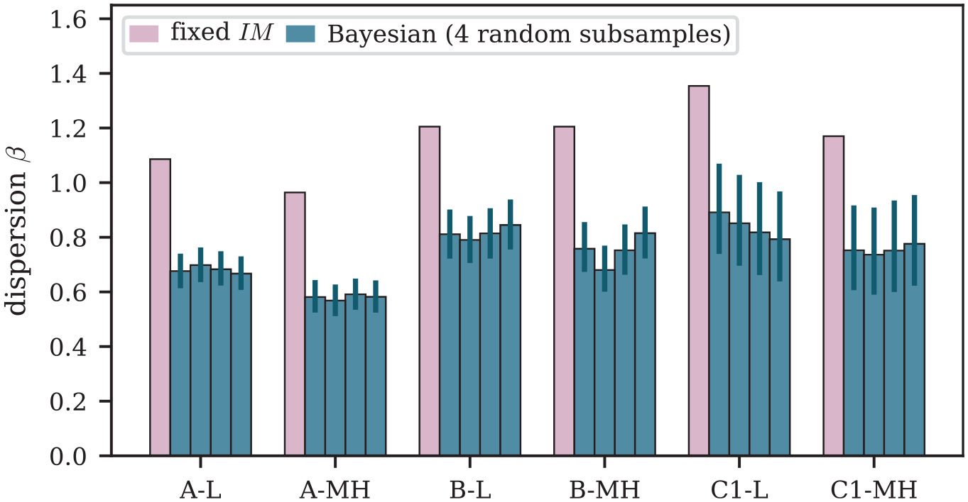
The proposed Bayesian approach is computationally expensive, and thus only one-fourth of the entire dataset is used for parameter estimation. This is a drawback compared to the fixed $\mathrm{IM}$ approach that handles the entire dataset with no computational difficulties and raises the question of how the Bayesian parameter estimates change for different subsets. Figure 10 shows $\beta$ values estimated with four randomly chosen sub-samples of the entire dataset. The four estimated values for each building class are within the posterior distribution CIs, and with differences that are much less than the difference relative to the fixed $\mathrm{IM}$ values, indicating that the proposed approach produces stable outputs even with random sub-sampling. This is perhaps not surprising given the large number of observations that remain within a given sub-sample. Recall that we randomly selected 25% of the data points from each building class/damage state combination shown in Table 2. The use of more sophisticated sub-sampling techniques is likely to further reduce the sensitivity of the estimated parameters.

Figure 10.

Comparison of estimated $\beta$ values from the fixed $\mathrm{IM}$ approach and for MCMC estimated from four random sub-samples of the entire dataset.

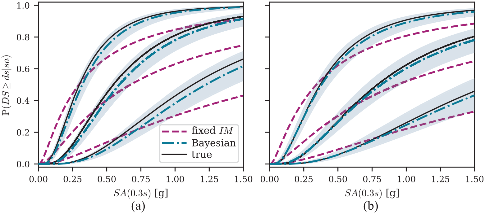
In a separate analysis, we compare the performance of both estimation methods in recovering a set of known, “true,” fragility functions while using the same sub-sampling technique as above. For this purpose, we replace the observed damage states in the L’Aquila dataset by simulated values. These are obtained by first drawing one sample of $\mathbf{i}{\mathbf{m}}_{\mathcal{B}}$ from the established conditional distribution $p(\mathbf{i}{\mathbf{m}}_{\mathcal{B}}|\mathbf{i}{\mathbf{m}}_{\mathcal{S}},\mathbf{rup})$ and then using a pre-defined set of fragility functions to sample a damage state for each building. Figure 11 compares the estimated fragility functions of two building classes, A-L and B-MH, to the “true” data-generating functions. For better readability, we only plot the functions for $\mathrm{ds}\in \{1,2,4\}$ . The functions obtained from the fixed $\mathrm{IM}$ approach are flatter than the “true” functions, while the Bayesian approach leads to functions that are in good agreement, despite only one-fourth of the dataset being used.

Figure 11.

Comparison of fragility functions of building class (a) A-L and (b) B-MH estimated from a simulated version of the L’Aquila damage survey dataset to the “true” data-generating functions. For better readability, only functions for $\mathrm{ds}\in \{1,2,4\}$ are plotted (from top left to bottom right).

Conclusion

This study explored the role of $\mathrm{IM}$ uncertainty in the estimation of fragility function parameters from damage survey data gathered after earthquake events and proposed a novel estimation method that can account for this uncertainty. Traditional estimation methods do not allow to account for such uncertainty and instead assume fixed, deterministic, $\mathrm{IM}$ values. In simulated case studies, traditional methods reportedly failed to recover the “true” data-generating fragility functions. To address this shortcoming, we proposed a Bayesian estimation approach that simultaneously considers $\mathrm{IM}$ values and fragility function parameters as uncertain variables. We derived an expression for their joint distribution conditional on the gathered damage data. For parameter estimation, we approximate this posterior distribution through MCMC sampling.

We applied the proposed method in a case study using damage data gathered after the 2009 L’Aquila earthquake event. The dataset consists of 56,400 residential masonry buildings that are categorized into six building classes and for which overall damage is described with six categories ranging from no damage to collapse.

We used both synthetic data and the L’Aquila data to compare the Bayesian parameter estimates with estimates from a traditional, fixed $\mathrm{IM}$ , approach. The two methods produce surprisingly different fragility functions, with those obtained from the fixed $\mathrm{IM}$ approach being flatter than their counterparts derived with the proposed Bayesian approach. The flatter fragility functions predict higher probabilities of damage for low $\mathrm{IM}$ values and, conversely, lower probabilities for high $\mathrm{IM}$ values. Such behavior is observed across all damage states and building classes. By fixing $\mathrm{IM}$ values to best-estimate values, the variability of the actual, unobserved, $\mathrm{IM}$ values around these best estimates manifests in an increased apparent dispersion in the estimated fragility functions. The proposed Bayesian approach, however, explicitly accounts for both variability sources and performs joint inference on $\mathrm{IM}$ values and model parameters, which prevents such an inflation of fragility function dispersion.

Additional tests demonstrated that the proposed Bayesian approach is less sensitive to the choice of ground motion and spatial correlation models used to derive the distribution of $\mathrm{IM}$ conditional on station data (i.e. the ShakeMap) than the traditionally used method, which relies on fixed $\mathrm{IM}$ values. This reduced sensitivity is a significant advantage, as the $\mathrm{IM}$ predictions from any given ground motion and spatial correlation model are not “correct,” as must be assumed with the fixed $\mathrm{IM}$ method. The proposed method of jointly estimating the $\mathrm{IM}$ values and fragility parameters allows for more robust estimates with respect to such modeling assumptions.

The proposed Bayesian approach comes with computational challenges, in particular with respect to memory demand. The herein used computational infrastructure allowed performing inference for 14,000 data points. This number is sufficient for many damage datasets, but its application to the L’Aquila dataset required sub-sampling the dataset. To assess the implications of such sub-sampling, we performed two analyses. First, we found that the parameters estimated from multiple randomly chosen subsets were relatively stable across the different subsets. Second, we replaced the observed damage with simulated values and found that the Bayesian approach could recover the “true” data-generating fragility functions using only a subset of the data. The fixed $\mathrm{IM}$ approach, however, failed to do so even when the entire dataset was used for parameter estimation. While the proposed method does require an additional analyst effort and more computational resources relative to the traditional estimation method, the required effort is still vastly smaller than the time and cost of inspections to collect the damage data, and so is a good investment given the extra value it provides.

While the focus of the presented work lies on $\mathrm{IM}$ uncertainty, the proposed method can be extended to account for uncertainties in other model inputs, such as missing database entries. The method could also be adapted to fragility models that have different dispersion parameters for each damage level and depend on building characteristics in a more complex manner than the commonly used categorization into pre-defined building classes. Despite these opportunities for further research, the novel estimation method can already be of substantial benefit for analysts interested in improved empirical fragility modeling. For the above reasons, we strongly believe that the method’s presented comparative advantages justify its increased computational complexity.

Supplemental Material

sj-pdf-1-eqs-10.1177_87552930241261486 – Supplemental material for Accounting for ground-motion uncertainty in empirical seismic fragility modeling

Supplemental material, sj-pdf-1-eqs-10.1177_87552930241261486 for Accounting for ground-motion uncertainty in empirical seismic fragility modeling by Lukas Bodenmann, Jack W Baker and Božidar Stojadinović in Earthquake Spectra