Sage Journals: Discover world-class research

Abstract

Following an earthquake, ground motion time series are needed to carry out site-specific nonlinear response history analysis. However, the number of currently available recording instruments is sparse; thus, the ground motion time series at uninstrumented sites must be estimated. Tamhidi et al. developed a Gaussian process regression (GPR) model to generate ground motion time series given a set of recorded ground motions surrounding the target site. This GPR model interpolates the observed ground motions’ Fourier Transform coefficients to generate the target site’s Fourier spectrum and the corresponding time series. The robustness of the optimized hyperparameter of the model depends on the surrounding observation density. In this study, we carried out sensitivity analysis and tuned the hyperparameter of the GPR model for various observation densities. The 2019 M7.1 Ridgecrest and 2020 M4.5 South El Monte earthquake data sets recorded by the Community Seismic Network and California Integrated Seismic Network in Southern California are used to demonstrate the process. To provide a tool to quantify the uncertainty of the generated motions, a methodology to develop realizations of ground motion time series is also incorporated. The results illustrate that the uncertainty of the generated motions is lower at longer periods. It is shown that the observation density in the proximity of the target site plays a vital role in both error and uncertainty reduction of the generated time series. To demonstrate the concept, the effect of additional observations from combined recording networks is investigated.

Keywords

Ground motion simulation Gaussian process regression uncertainty quantification conditioned ground motions

Introduction

The current number of ground-level recording instruments is approximately 2000 in California over multiple recording networks (Southern California Earthquake Data Center, 2022). Consequently, following a major event, ground motion time series at locations devoid of recording instruments are needed to carry out site-specific nonlinear response history analysis. Currently, important products “ShakeCast” and “ShakeMap” established by US Geological Survey (Fraser et al., 2008; Lin et al., 2018; Wald et al., 2008; Worden et al., 2018) provide ground motion intensity measures (GMIM), such as peak ground acceleration and response spectral ordinates. However, as stated above, ground motion time series at uninstrumented sites are also required for seismic performance evaluation of specific structures.

Two commonly used methodologies for generating ground motion time series at uninstrumented sites can be mentioned here. First, the physics-based simulations employing the finite-fault and seismic velocity models consider the source, path, and site effects (e.g. Aagaard et al., 2008; Atkinson and Assatourians, 2015) and the topography of the Earth’s surface (Rodgers et al., 2019; Thomson et al., 2020). Second, the coherency function-based simulations employing cross-spectral density (CSD) and auto-spectral density (ASD) functions (e.g. Kameda and Morikawa, 1992; Konakli and Der Kiureghian, 2012; Zentner, 2013; Rodda and Basu, 2018). Several research studies have also been conducted to simulate unconditional spatially varying ground motions. Deodatis (1996) and Shinozuka and Deodatis (1996) employed the spectral representation method (SRM) to simulate non-stationary stochastic ground motions. Furthermore, conditional simulation of non-stationary random fields was extensively investigated (Cui and Hong, 2020; Heredia-Zavoni and Santa-Cruz, 2000; Hu et al., 2012; Vanmarcke and Fenton, 1991; Wu et al., 2015). The physics-based approaches require detailed information regarding the subsurface properties and fault features. However, The CSDs are driven using empirical or semi-empirical coherency functions, whose coefficients are often determined via data-driven methods (Abrahamson et al., 1991). The CSD functions might need some detailed site properties and wave propagation characteristics. Therefore, both methods have challenges for a rapid post-earthquake structural damage assessment in real time (Loos et al., 2020; Mangalathu and Jeon, 2020) as they are computationally expensive and time-consuming.

Tamhidi et al. (2021, 2022b) recently developed a method to simulate ground motion time series using a trained Gaussian process regression (GPR) model. This GPR model interpolates the discrete Fourier transform (DFT) coefficients of the observed nearby recorded ground motions to construct the time series at the target uninstrumented sites. The GPR model performs conditioned simulation of ground motions at an ensemble of target locations, imposing a comparatively low computational cost (Rasmussen and Williams, 2006).

The intrinsic uncertainty of ground motions affects earthquake engineering disciplines, such as the performance-based post-earthquake assessment and decision-making (Aghababaei et al., 2021; Roohi and Hernandez, 2020; Weatherill et al., 2015). Several studies attempted to quantify and model this randomness in various seismic problems (Alamilla et al., 2001; Wen et al., 2003; Yazdi et al., 2022). In this study, we focus on quantifying the uncertainty and validity of the generated motions using the GPR model introduced by Tamhidi et al. (2021). The model’s hyperparameter (the regularization factor) is fine-tuned based on observation densities, enabling the users to choose the optimum hyperparameter corresponding to the existing observed data set. Then, a methodology to generate random realizations of ground motions using the trained GPR and an inter-frequency correlation model (Bayless and Abrahamson, 2019) is reviewed. This random realization methodology provides a means to quantify the uncertainty of the generated motions at the target sites. We implemented this methodology to investigate the simulated motions’ accuracy and uncertainty using the 2019 M7.1 Ridgecrest earthquake data set recorded by the Community Seismic Network (CSN). In addition, the performance of the model as related to the spatial density of recording instruments is investigated for the 2019 Ridgecrest and 2020 M4.5 South El Monte earthquakes in Southern California.

Theoretical background

Suppose the ground motion acceleration time series at site s, a_s(t), is constructed with N discrete data points, a_s(t_i), i = 1, …, N. The time series can be decomposed into its DFT coefficients A_k (e.g. Oppenheim et al., 1997) as follows:

a_{s} (t_{i}) = \sum_{k = 0}^{N - 1} A_{k} e^{j ω_{k} t_{i}}

(1)

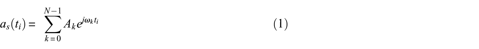
where

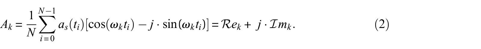
A_{k} = \frac{1}{N} \sum_{i = 0}^{N - 1} a_{s} (t_{i}) [\cos (ω_{k} t_{i}) - j \cdot \sin (ω_{k} t_{i})] = R e_{k} + j \cdot I m_{k} .

(2)

In Equations 1 and 2, $ω_{k}$ denotes the k^th DFT’s frequency and $j = \sqrt{- 1}$ . $R e_{k}$ and $I m_{k}$ are the DFT coefficient’s real and imaginary components at the k^th frequency, respectively. The DFT coefficients are assumed as random Gaussian variables, as demonstrated by Kameda and Morikawa (1992) and implemented by Konakli and Der Kiureghian (2012) to simulate ground motion fields. The $R e_{k}$ (or $I m_{k}$ ) at site s is correlated to $R {e_{k}}^{'}$ (or $I {m_{k}}^{'}$ ) at nearby sites $s^{'}$ . We implemented a GPR model to estimate $R e_{k}$ (and $I m_{k}$ ) given the observed $R {e_{k}}^{'}$ (and $I {m_{k}}^{'}$ ) at the neighboring sites. It is assumed that there is a statistically insignificant correlation between $R e_{k}$ (or similarly $I m_{k}$ ) and $R e_{j}$ (or similarly $I m_{j}$ ) at the same site for different frequencies k and j, when we construct the mean estimated ground motions. Tamhidi et al. (2021) showed that mean estimated values for a multivariate Gaussian variable (here $R e_{k}$ or $I m_{k}$ ) are independent of the inter-frequency correlation between amplitudes at different frequencies. However, this inter-frequency correlation must be taken into account if we want to generate random realizations of time series at a site.

Gaussian Process Regression

A Gaussian process (GP) is a set of indexed random variables, with every finite subset following multivariate Gaussian distribution (Rasmussen and Williams, 2006). The standard form of GP is shown in Equation 3:

f (x) ~ G P (m (x), k (x, x'))

(3)

In Equation 3, m( x ) represents the mean function value at the input vector location x , and k( x , $x^{'}$ ) is the covariance between vector locations x and $x^{'}$ . This article indicates vectors and matrices with lower-case and upper-case boldface symbols, respectively. Suppose there are $N_{o}$ and $N_{t}$ number of observed and target locations, respectively. We denote f as a $N_{o} \times 1$ vector of observed values from a GP and $f_{*}$ as a $N_{t} \times 1$ vector of unknown GP values at the target locations. Also, let us symbolize the observed locations’ $N_{o} \times d$ input matrix as X (d is the number of features for each location), whose rows contain observed locations’ input feature vectors, x . Similarly, we call $X_{*}$ as the $N_{t} \times d$ matrix of target locations. The predictive distribution of $f_{*}$ is given by (Rasmussen and Williams, 2006),

f_{*} | X_{*}, X, f ~ N (μ_{*}, Σ_{* *})

(4)

where

{μ_{*}}_{(N_{t} \times 1)} = μ_{(N_{t} \times 1)} + {K_{x_{*} x}}_{(N_{t} \times N_{o})} {K_{xx}^{- 1}}_{(N_{o} \times N_{o})} (f_{(N_{o} \times 1)} - μ_{(N_{o} \times 1)})

(5)

{Σ_{* *}}_{(N_{t} \times N_{t})} = {K_{x_{*} x_{*}}}_{(N_{t} \times N_{t})} - {K_{x_{*} x}}_{(N_{t} \times N_{o})} {K_{xx}^{- 1}}_{(N_{o} \times N_{o})} {K_{x x_{*}}}_{(N_{o} \times N_{t})}

(6)

In Equation 4, $μ_{*}$ and $Σ_{* *}$ stands for the posterior mean vector and covariance matrix of the GP values at target locations, respectively. In Equations 5 and 6, $μ$ denotes a vector of GP prior mean; K _xx and $K_{x_{*} x_{*}}$ are the covariance matrix of the DFT coefficients at the observed and target locations, respectively. Correspondingly, $K_{x x_{*}}$ (transpose of $K_{x_{*} x}$ ) represents the covariance between the observed and predicted DFT coefficients. The covariance matrices’ elements are constructed with covariance kernel, k(r), where r denotes the distance between input vectors. Tamhidi et al. (2021) indicated that the Matérn kernel with $ν = 1.5$ is the optimum covariance function for the GPR model to simulate the ground motion time series. Equations 7 and 8 illustrate Matérn ( $ν$ = 1.5) kernel function and the “distance” between two input vectors, $x$ and $x^{'}$ , respectively. The “distance” can be the geographical distance and the difference between local soil conditions ( $V_{s_{30}}$ ) at two sites as elaborated below.

k_{ν = 1.5} (r) = σ_{f}^{2} (1 + \sqrt{3} r) \exp (- \sqrt{3} r)

(7)

r = θ \sqrt{\sum_{i = 1}^{d} {(x_{i} - {x^{'}}_{i})}^{2}}

(8)

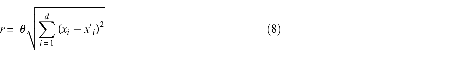
In Equation 7, $σ_{f}$ is the variance that governs how uncertain the GPR’s estimate is. In Equation 8, $x_{i}$ is the i^th component of the input vector at location x and $θ$ is a positive scaling factor, as the inverse of length-scale, l, where $θ = \frac{1}{l}$ . The length-scale, l, is a parameter of the covariance function, which scales the “distance” between two locations. In other words, a larger length-scale results in a higher correlation by reducing the “distance.” In this study, all input vector’s elements are scaled with the same $θ$ . Such a covariance function is called an isotropic covariance function.

Tamhidi et al. (2020, 2021) demonstrated that a four-dimension input vector, $x = {x_{1}, x_{2}, x_{3}, \log (V_{s_{30}})}$ , is appropriate to represent sites. $V_{s_{30}}$ is the time-average shear wave velocity in the uppermost 30 m of the soil, and x₁ through x₃ are the Cartesian coordinates of the site on the 3D surface of the Earth. All four input attributes are normalized, so that each feature’s mean and standard deviation are zero and one, respectively. The GPR model’s parameters are the distance scaling factor, $θ$ , the GP prior mean, $μ$ , and the variance, $σ_{f}$ , which need to be optimized for each $R e_{k}$ (and $I m_{k}$ ) at the target site using the observations which are all known ground motions $R {e_{k}}^{'}$ (and $I {m_{k}}^{'}$ ) within the corresponding event’s data set. The maximum a posteriori estimates are chosen as the optimum model’s parameters by maximizing the penalized log-likelihood of the observations. Denoting the parameters as $γ = (θ, μ, σ_{f})$ , Equation 9 displays the penalized log-likelihood of the observations:

Q (γ) = - \frac{1}{2} {(f - μ)}^{T} {K_{xx}}^{- 1} (f - μ) - \frac{1}{2} \log | K_{xx} | - \frac{N_{o}}{2} \log 2 π - N_{o} d p_{λ} (θ)

(9)

In Equation 9, T stands for the transpose operator and $p_{λ} (θ)$ is a non-negative penalty function for the scaling factor $θ$ . This study uses the L2 penalty function shown in Equation 10.

p_{λ} (θ) = λ θ^{2}

(10)

The regularization factor, $λ$ , is the hyperparameter of the model that determines how observations contribute the optimum parameters, $\hat{γ}$ .

Hyperparameter optimization

A higher penalty is needed when there are sparse observations (Li and Sudjianto, 2005). In other words, the optimum hyperparameter, $\hat{λ}$ , depends on the observation density. Thus, it is required to tune the $\hat{λ}$ for various observation densities. We used the recorded ground motions of the 2019 M7.1 Ridgecrest earthquake by the CSN within Los Angeles (Clayton et al., 2020).

The observation density for the 252 CSN recording sites distributed over a 464 km² region (CSN domain in Figure 1) is 0.54 sites/km². To tune the optimum $\hat{λ}$ for various observation densities, we make different data sets with the various number of observed sites by randomly selecting out of the 252 CSN sites. Six different data sets with 252, 201, 151, 100, 50, and 25 sites are chosen. The distribution of the randomly chosen subsets is shown in Figure 1. The $V_{s_{30}}$ values of the CSN sites are estimated using a proxy-based model described in Ahdi et al. (2020). The selection criterion for finding $\hat{λ}$ is to minimize the average normalized root mean square error (NRMSE) between the recorded and generated ground motions’ 5%-damped RotD50 response spectra (Boore, 2010). The NRMSE between the recorded and estimated motions’ response spectra is calculated by Equation 11.

NRMSE = \sqrt{\frac{1}{N_{p}} \sum_{i = 1}^{N_{p}} \frac{{(PS A_{i} - {\hat{PSA}}_{i})}^{2}}{{\hat{PSA}}_{i}^{2}}}

(11)

Figure 1.

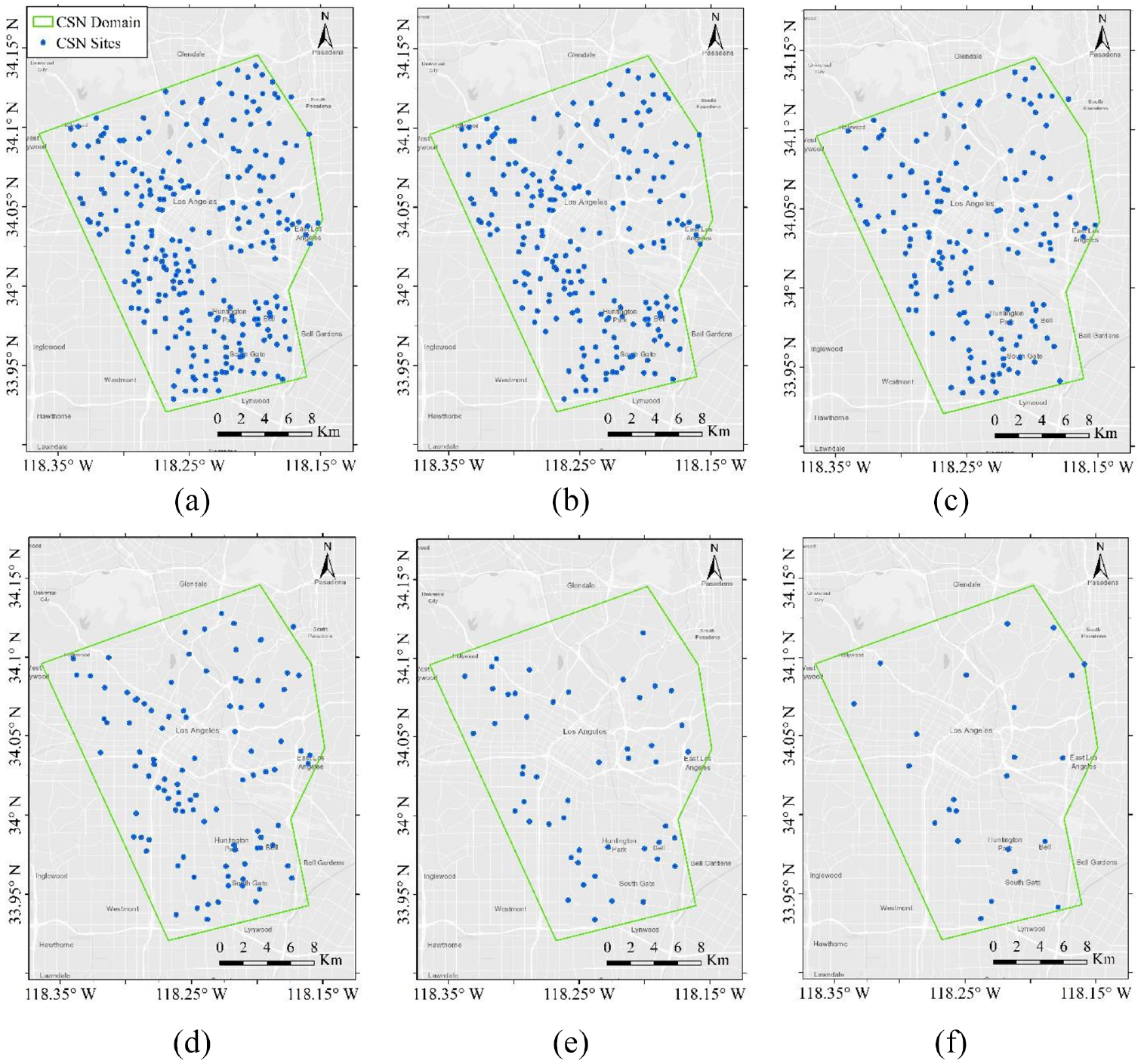
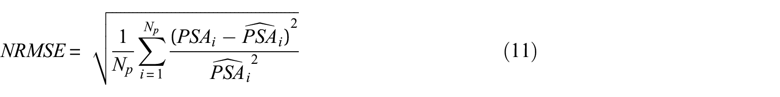
Distribution of the randomly chosen subsets from CSN’s recorded 2019 M7.1 Ridgecrest earthquake motions with (a) 252, (b) 201, (c) 151, (d) 100, (e) 50, and (f) 25 number of sites.

In Equation 11, $PS A_{i}$ and ${\hat{PSA}}_{i}$ are the response spectral ordinates of the estimated and recorded ground motions at the i^th period, respectively, and $N_{p}$ equals to the number of periods included within the usable bandwidth. The usable bandwidth is considered as the mutual usable bandwidth among all observed motions, which is the reliable period range after the noise removal of the motions (Ancheta et al., 2014). We implemented the Leave-One-Out (LOO) cross-validation methodology (Vehtari et al., 2017) to find $\hat{λ}$ for each subset shown in Figure 1. Nine different regularization factors, 0.01, 0.02, 0.05, 0.1, 0.2, 0.4, 0.6, 0.8, and 1.0, called as $λ_{test}$ , are examined for each subset through the following steps to find the $\hat{λ}$ . These $λ_{test}$ values are chosen, so that the $\hat{λ}$ for each subset falls inside the 0.01–1.0 domain (cf. Table 1).

1. For each site, s, within the data set, s = 1,…, N_sites (N_sites = number of sites in the data set)

1.1. Obtain the optimum parameters $\hat{γ}$ at the k^th frequency using the observed ground motions, which are all the recorded ground motions (excluding at site s) by maximizing $Q (γ_{k})$ using $λ_{test}$ .

1.2. Generate the ground motion time series at site s using posterior mean (Equation 5) of $R e_{k}$ and $I m_{k}$ , $k = 0, \dots, N - 1$ , given $\hat{γ}$ in Step 1.1. We call this generated time series the mean estimated ground motion.

1.3. Obtain the RotD50 spectrum of the mean estimated and recorded ground motions at site s and calculate NRMSE between them, called as Error_s.

2. Compute the average of Error_s among all sites, s = 1, …, N_sites, and store it as Error_avg corresponding to $λ_{test}$ .

Eventually, the $λ_{test}$ corresponding lowest Error_avg is chosen as $\hat{λ}$ associated with the target data set’s observation density. Table 1 illustrates the obtained $\hat{λ}$ for each data set and the corresponding Error_avg for the mean estimated ground motions.

Table 1.

The optimum regularization factor, $\hat{λ}$ , and corresponding Error_avg for various observation densities

No. of observation	Density (station/km²)	$\hat{λ}$	Average RotD50 NRMSE (Error_avg)
251	0.54	0.05	0.27
200	0.43	0.1	0.28
150	0.32	0.1	0.27
99	0.21	0.1	0.31
49	0.10	0.2	0.30
24	0.05	0.4	0.40

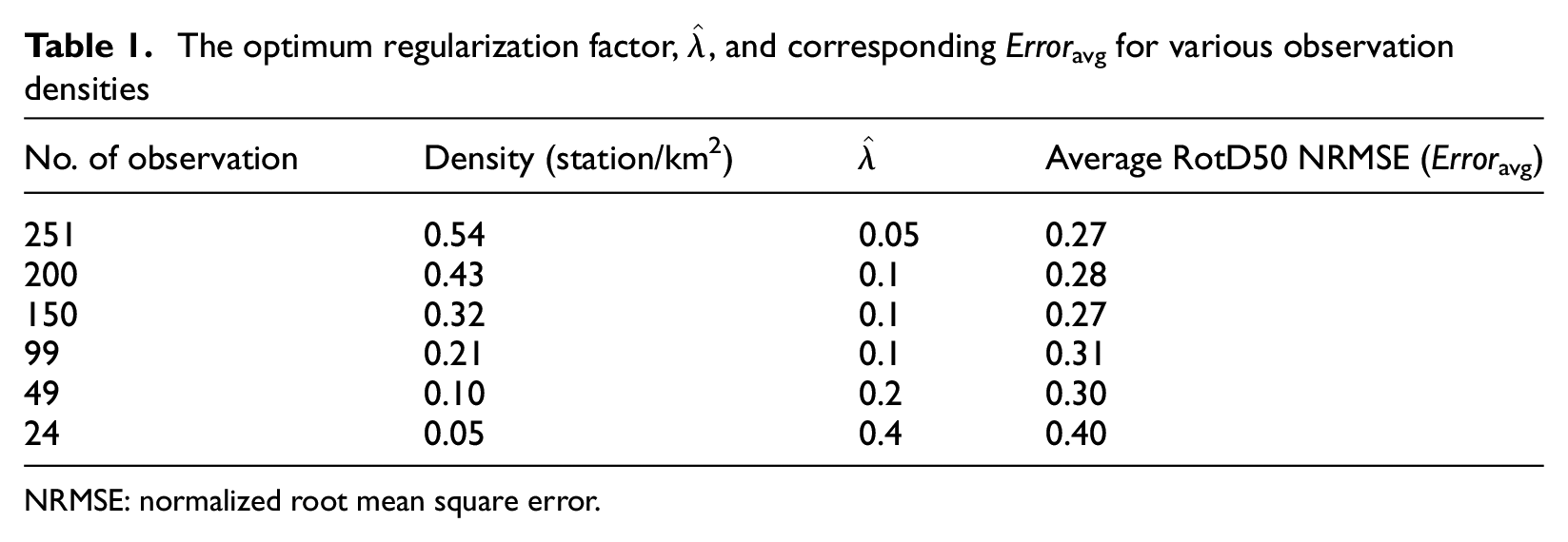
NRMSE: normalized root mean square error.

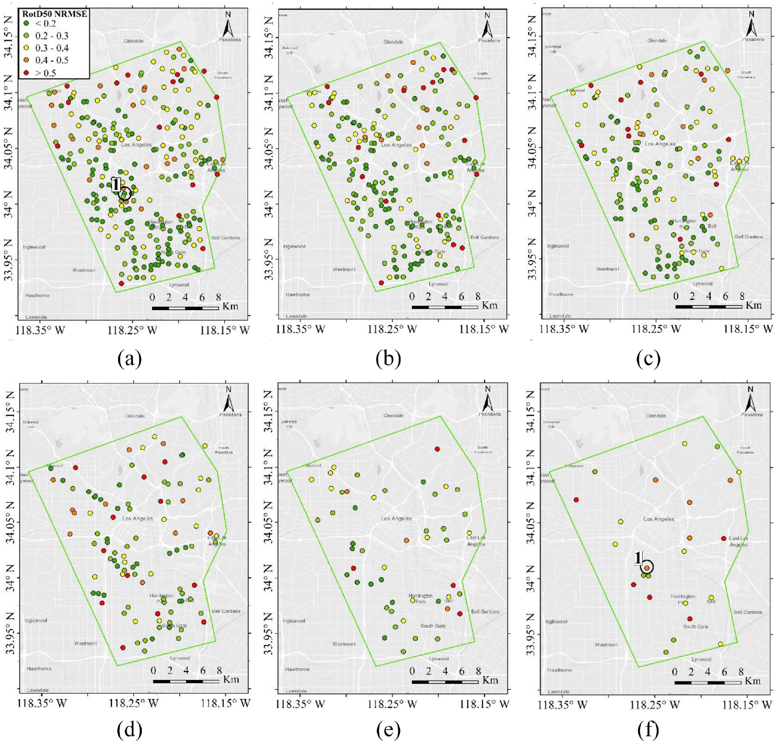
We have employed the $\hat{λ}$ given in Table 1 to generate the mean estimated ground motion time series using LOO analysis at each site within the corresponding data set. Figure 2 depicts the distribution of the NRMSE between the recorded and mean estimated ground motions’ RotD50 spectrum. It is demonstrated that the predicted ground motions are reliably accurate for most of the target sites for the subsets with higher observation density (cf. Figures 2a, through c). However, the Error_avg increases as observation density decreases (cf. Figures 2d through f). The effect of observation density on the prediction accuracy and uncertainty is examined in further depth in section “Uncertainty quantification and sensitivity analysis.”

Figure 2.

Distribution of the RotD50 NRMSE between the recorded and mean estimated ground motions using corresponding $\hat{λ}$ for CSN sites recorded M7.1 Ridgecrest earthquake having (a) 251, (b) 200, (c) 150, (d) 99, (e) 49, and (f) 24 number of observed sites. The Test Site 1 (panels a and f) is chosen as a target site for the assessment of the introduced methodology for random generation of ground motions (see section “Ground motion random realizations”).

Ground motion random realizations

It is desirable to quantify the uncertainty of the mean estimated ground motions at any target site. The posterior mean vector and covariance matrix for all target sites’k^th frequency DFT coefficients, k = 0, …, N−1, are given by Equations 5 and 6. In this study, we generate ground motion time series at one target site at each process. Therefore, Equations 5 and 6 can be converted to Equations 12 and 13, providing the scalar posterior mean, $μ_{*}$ , and standard deviation, $σ_{*}$ , for each $R e_{k}$ (and $I m_{k}$ ):

μ_{*} = \hat{μ} + {k_{x_{*} x}}_{(1 \times N_{o})} {K_{xx}^{- 1}}_{(N_{o} \times N_{o})} (f_{(N_{o} \times 1)} - μ_{(N_{o} \times 1)})

(12)

σ_{*} = \hat{σ_{f}} - {K_{x_{*} x}}_{(1 \times N_{o})} {K_{xx}^{- 1}}_{(N_{o} \times N_{o})} {K_{x x_{*}}}_{(N_{o} \times 1)}

(13)

In Equations 12 and 13, $k_{x_{*} x}$ is the vector of covariance among the target site and observed sites $R e_{k}$ (or $I m_{k}$ ). $k_{x_{*} x}$ and $K_{xx}$ are established using $\hat{γ}$ at the corresponding frequency. The ground motion realizations at each target site are generated following below steps:

At each k^th frequency, k = 0, …, N−1:

1.1. The posterior mean and standard deviation of $R e_{k}$ and $I m_{k}$ are calculated by Equations 12 and 13.

1.2. The correlation between the $R e_{k}$ and $I m_{k}$ at the target site is estimated by the correlation between $R {e_{k}}^{'}$ and $I {m_{k}}^{'}$ among all observed sites’ (whole data set except target site) ground motions. Consequently, a 2 × 2 covariance matrix for the ( $R e_{k}$ , $I m_{k}$ ) is established using the estimated correlation and standard deviations resulted in Step 1.1.

1.3. A set of random samples of 2 × 1 vectors of ( $R e_{k}$ , $I m_{k}$ ) are produced using the estimated 2 × 1 mean vector (Step 1.1) and 2 × 2 covariance matrix (Step 1.2). The sample size is selected so that the average of the generated samples becomes stable and converges to the mean vector determined in Step 1.1. These generated ( $R e_{k}$ , $I m_{k}$ ) are then transformed to $| A_{k} |$ samples.

1.4. The logarithmic mean and standard deviation of $| A_{k} |$ samples in Step 1.3 are obtained.

The N × N covariance matrix of $\log (| A_{k} |)$ , k = 0, …, N−1, are constructed using the inter-frequency correlation values given by Bayless and Abrahamson (2019) model and calculated standard deviations in Step 1.4.

Random Gaussian N × 1 vector samples of $\log (| A_{k} |)$ are produced using the N × 1 mean vector (Step 1.4) and N × N covariance matrix (Step 2).

The phase spectrum of the mean estimated ground motion is coherent with the nearby observed ground motions. Therefore, the generated samples of Fourier amplitude spectrum (FAS) in Step 3 are combined with the Phase spectrum constructed with the posterior mean DFT coefficients to generate ground motion time series realizations.

We also examined the randomization of Fourier phase spectra; yet, the results were not as promising as the outcomes stated in Step 4 above. We employ the 2019 M7.1 Ridgecrest earthquake data set recorded over the CSN sites to evaluate the proposed methodology. Test Site 1 shown in Figures 2a and f is the target site. The geotechnical properties of Test Site 1 are summarized in Table 2. In Table 2, Z_1.0 and Z_2.5 are depths to the V_s = 1 km/s and V_s = 2.5 km/s horizons, respectively, and are estimated using the SCEC CSM-S4 model (Nweke et al., 2018). In Table 2, R_rup is the closest distance to the coseismic rupture.

Table 2.

Site properties of the Test Site 1 shown in Figure 2

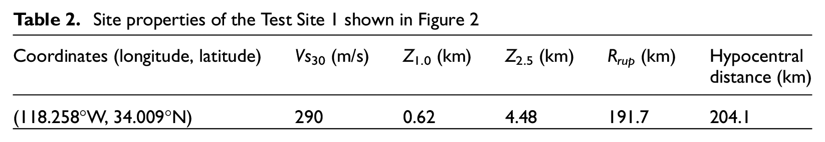
Coordinates (longitude, latitude)	Vs₃₀ (m/s)	Z_1.0 (km)	Z_2.5 (km)	R_rup (km)	Hypocentral distance (km)
(118.258°W, 34.009°N)	290	0.62	4.48	191.7	204.1

Two different observed sets are considered to generate ground motion realizations at Test Site 1; first, all 251 CSN sites in Figure 2a, and second, all 24 CSN sites in Figure 2f. The $\hat{λ}$ for each case is chosen from Table 1. We generated 100 ground motion realizations at Test Site 1. Figure 3 indicates the mean estimated and five ground motion time series realizations along the East–West (EW) direction at the Target Site 1. Figure 3a displays that the mean estimated and generated realizations of ground motion given 251 observed sites fit closer to the recorded one than those estimated using 24 observed sites in Figure 3b. In addition, it is observed from Figure 3a that the generated ground motion time series using 251 observed sites exhibit minor variation (uncertainty) at long periods (cf. velocity and displacement time series in Figure 3a). However, the higher frequency content of the generated motions shows a greater degree of uncertainty even using 251 observations (cf. accelerations in Figure 3a). However, Figure 3b displays that 24 observed sites are insufficiently informative to estimate the long-period content of the motions (cf. velocity and displacement time series in Figure 3b). The reason for this is because the average distance between the 24 observed sites is not close enough to predict long waves of the motion.

Figure 3.

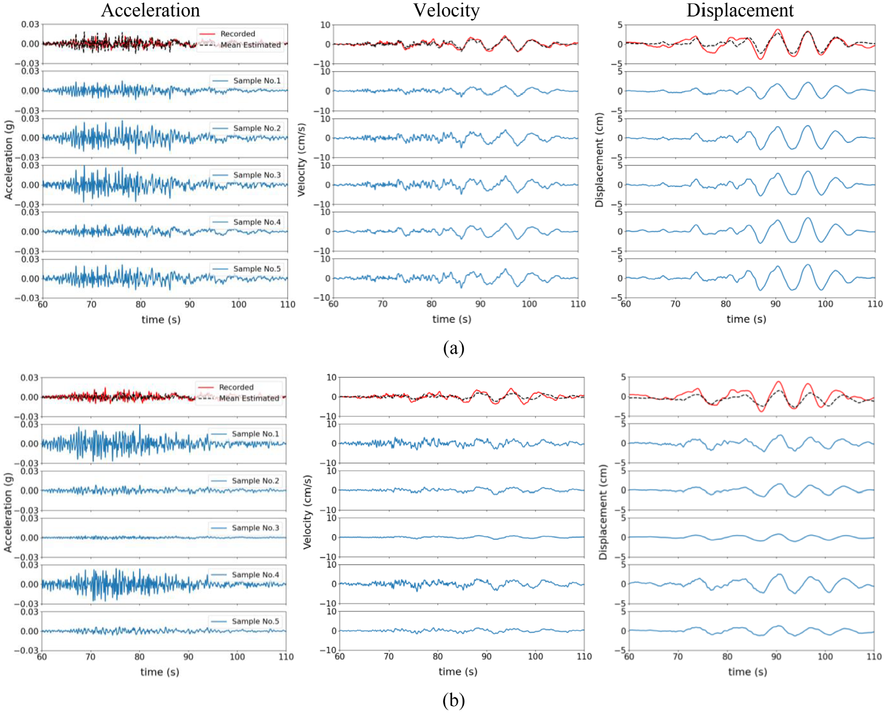
Estimated mean and five generated ground motion realizations time series along EW direction at the Test Site 1 within the M7.1 Ridgecrest earthquake CSN data set shown in Figures 2a and f using (a) 251 and (b) 24 observed sites.

Figure 4 depicts the mean estimated and 100 ground motion realizations’ 5%-damped RotD50 spectra at Test Site 1 using 251 and 24 observed sites. It is acknowledged that the generated motions’ uncertainty is lower at long periods than those at short periods. Moreover, Figure 4 indicates that the long-period prediction (longer than 1 s) has minor variation and error for having 251 observed sites than those estimated with 24 observations. However, neither 251 nor 24 observations are dense enough to provide informative detail of short-length waves corresponding to the short periods. That is why it is seen in Figures 4a and b that the short periods’ variation is high and does not differ significantly from having 251 observations to 24 ones.

Figure 4.

The 5%-damped RotD50 spectrum of generated ground motion realizations at the Test Site 1 using the (a) 251 (Figure 2a) and (b) 24 (Figure 2f) observed sites.

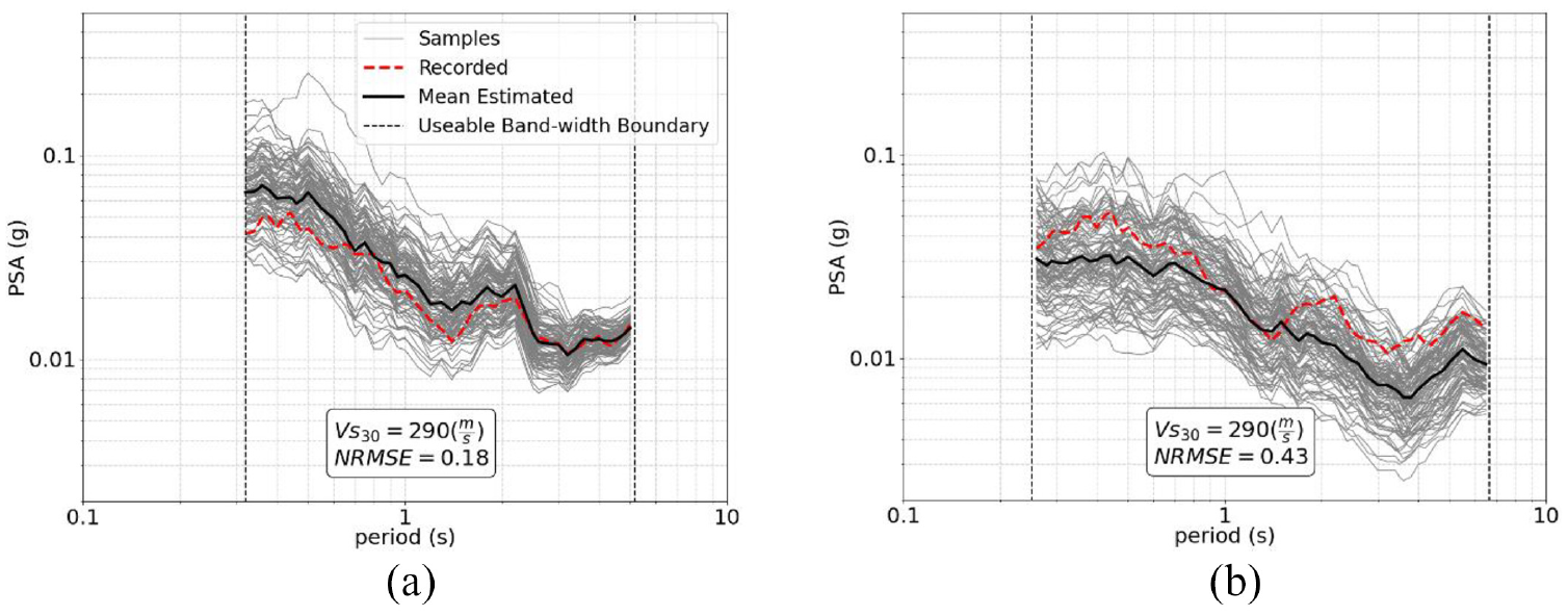
Figure 5 presents the 68% confidence interval (CI), mean ± standard deviation, for the RotD50 spectra of generated realizations at Test Site 1 employing 251 and 24 observed sites. In addition, Figure 5 demonstrates the average RotD50 spectrum provided by CB14 (Campbell and Bozorgnia, 2014), ASK14 (Abrahamson et al., 2014), and BSSA14 (Boore et al., 2014) ground motion models (GMMs) and their average within-event standard deviation.

Figure 5.

The 68% CI of RotD50 spectrum of generated ground motion realizations at the Test Site 1 using the (a) 251 (Figure 2a) and (b) 24 (Figure 2f) observed sites.

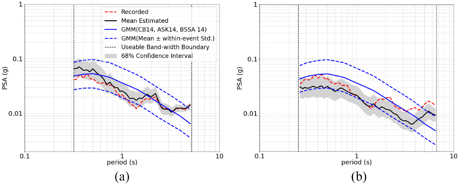
Figure 5a indicates that the recorded ground motion response spectrum falls inside 68% CI of the generated motions using 251 observations for the majority of periods. Furthermore, Figure 5a shows that within-event uncertainty for the average GMMs is greater than that of generated motions using 251 observations. Figure 5a also displays that the logarithmic CI of the estimated motions narrows at longer periods. In contrast, the within-event standard deviation of GMMs does not change considerably. In other words, the estimated ground motions’ variability is less than that of GMMs, especially at long periods. However, Figure 5b demonstrates that the recorded ground motion response spectrum falls either outside or on the edge of 68% CI for having 24 observed sites. In addition, Figure 5 indicates that the standard deviation from short to long periods does not alter considerably for having fewer observations. Interested readers are referred to Tamhidi et al. (2022a) to know more about the observation density’s effect on 68% CI of estimated motions at other target sites of CSN.

Uncertainty quantification and sensitivity analysis

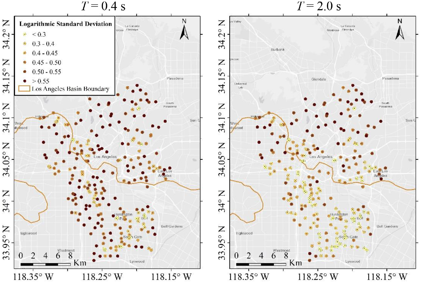
Accuracy and uncertainty of the generated time series are quantified in this section. We employed 252 CSN sites’ LOO analysis results for the 2019 M7.1 Ridgecrest earthquake. The logarithmic standard deviation of 100 generated pseudo-spectral accelerations (PSAs) at two periods, T = 0.4 and 2.0 s, is obtained as a measure of generated motions’ uncertainty at short and long periods, respectively. Figure 6 depicts the distribution of the EW PSAs’ logarithmic standard deviation at T = 0.4 and 2.0 s.

Figure 6.

The PSA logarithmic standard deviation of the estimated ground motions along EW direction at two periods T = 0.4 and 2.0 s for the M7.1 Ridgecrest earthquake CSN data set.

Figure 6 illustrates that estimated ground motion realizations at CSN sites on the Los Angeles basin show minor variations at long periods (T = 2.0 s) compared to those located outside the basin. However, the generated motions’ uncertainty at short period, T = 0.4 s, changes insignificantly between CSN sites inside and outside the Los Angeles basin. Comparing results at T = 0.4 with 2.0 s in Figure 6 reveals that the PSA’s logarithmic standard deviation at long period is smaller than those of short period for sites located on the basin. However, the PSA logarithmic standard deviation does not vary considerably from the short to the long period for sites located outside the basin. This is primarily because the observation density surrounding the target sites in southern part of the CSN is high enough to produce reliable long-period motions. Furthermore, the sites atop the Los Angeles basin receives more coherent long-period motions as evidenced by Kohler et al. (2020). Thus, the estimated motions at long periods are less uncertain for the target sites on the basin.

As a metric of observation density surrounding each target site, we determined the average distance (inside the 4D space established in previous sections) between each target site and its four nearest observed neighbors. In this article, we refer to this distance as “average separation distance.” The shorter average separation distance indicates a higher observation density surrounding the target site. Figure 7 depicts the scatter plot of the mean estimated motions’ PSA NRMSE within usable bandwidth along EW, North–South (NS), and RotD50 concerning the average separation distance. Figure 7 also depicts the fitted lines to the scatter plots and their R-squared, R². The separation distance in Figure 7 is unitless as the feature vectors are all normalized, as elaborated in the “Theoretical background” section.

Figure 7.

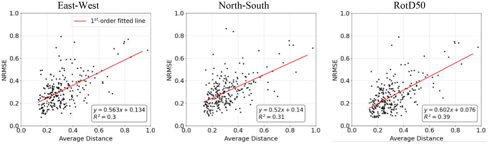
Scatter plot of the PSA NRMSE with respect to the average separation distance for the 2019 M7.1 Ridgecrest earthquake CSN data set.

Figure 7 shows that estimation error and average separation distance have a general direct correlation. One can recognize that having more observations closer to the target site results in more accurate ground motion prediction, as expected and now quantified in Figure 7. Figure 8 indicates the scatter plot of the PSA’s logarithmic standard deviation along EW and NS at T = 0.4 and 2.0 s relative to the average separation distance. Figure 8 displays that the estimation uncertainty at T = 2.0 s grows as the average separation distance increases. In addition, it is noticeable that in a general trend, the uncertainty of the long-period estimation is sensitive to the observation density; but, the short-period estimation (T = 0.4 s) is not significantly correlated with the number of observations surrounding the target site. This phenomenon is due to the complexities and intrinsic unpredictability of the short-period motions, making added observations less useful to produce reliable short-period waves. Comparing the scatter plots at T = 0.4 and 2.0 s in Figure 8 reveals that the long-period motions have less variability than short-period ones at shorter average separation distances. Figure 8 demonstrates that for a target site with average distance of 0.2 from its four nearest neighbors, the estimated logarithmic standard deviation for PSA is around 0.45 and 0.30 at T = 0.4 and 2.0 s, respectively. Furthermore, Figure 8 depicts that both short and long periods’ uncertainty saturates for very long average separation distances. In other words, the GPR model produces random estimations with similar variance at short and long periods where there are too few observations.

Figure 8.

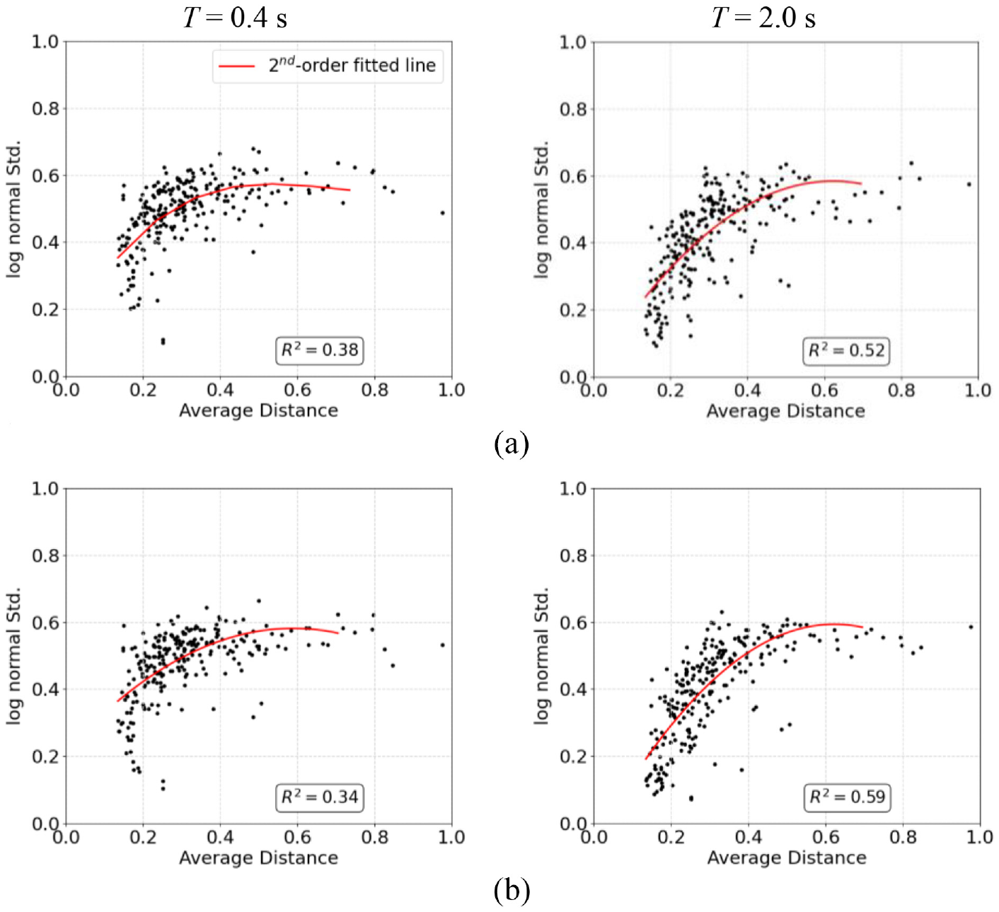
Scatter plot of the logarithmic standard deviation of PSA along (a) EW and (b) NS for the M7.1 Ridgecrest earthquake CSN data set.

Figure 9 demonstrates the stacked bar plots for the proportion of target sites where the recorded PSA falls inside (or outside) the estimated motions’ 68% CI with regard to the average separation distance. The eight spans of average separation distance shown in Figure 9 are selected so that each span includes an approximately same number of target sites. Figure 9 indicates that the percentage of sites where the recorded PSA locates outside of the 68% CI rises as average separation distance grows. This pattern becomes more apparent at T = 2.0 s. The percentage of sites where their 68% CI includes the recorded PSA decreases steadily for average distances greater than 0.3 and 0.2 for T = 0.4 and 2.0 s, respectively.

Figure 9.

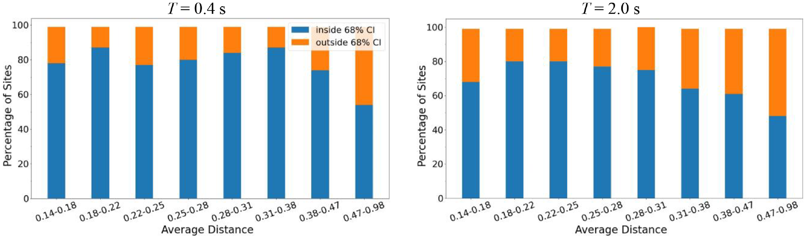
Stacked bar plots of the percentage of target sites where the EW recorded PSA falls inside the 68% CI with respect to average separation distance for 2019 M7.1 Ridgecrest earthquake CSN data set.

Consequently, it may be concluded that the target sites with higher observation densities close to them are more likely to have the recorded PSA within their 68% CI estimation. About 76% and 74% of the 252 target sites’ estimated PSA at T = 0.4 s captures the recorded one within 68% CI along EW and NS, respectively. Similarly, 70% and 76% of the target sites’ generated PSA at T = 2.0 s includes the recorded spectral ordinate within 68% CI along EW and NS, respectively. The effect of other governing parameters, such as uncertainty of the predicted site conditions ( $V_{s_{30}}$ ) and the surface slope of the nearby instrumented sites on estimations, is studied by Tamhidi et al. (2022a).

In summary, Figure 8 shows that increasing the density of instrumentation closer to the target site reduces the variability of the generated ground motions. As a result, the higher observation density is expected to decrease uncertainty of structural engineering demand parameters derived from nonlinear response history analyses. Figure 9 indicates that for the target sites with a greater observation density, the uncertainty of long-period estimated motions is smaller than that for short periods; however, the probability that the recorded spectrum falls within 68% CI is almost the same at both short and long periods. In other words, for target sites with average distances shorter than 0.3, the PSA realizations are about 80% likely to capture the recorded spectra within their mean ± standard deviation bandwidth.

Performance evaluation on combined network data sets

Herein, we study the potential improvement of the ground motion prediction using combined observations from different seismic networks. There are various seismic networks in California, and the combined network is called California Integrated Seismic Network (CISN). First, we execute LOO ground motion prediction at each CISN station as a target site using all other CISN sites (except the target site) as observation. Second, we perform the same procedure to estimate the ground motion time series at each CISN site using all other CISN and CSN sites as observation. Comparing the predicted motions resulting from these two observed sets with the recorded ones reveals the improvement of the GPR model’s output. Ground motions recorded in two recent earthquakes are employed for this purpose: (1) 2019 M7.1 Ridgecrest and (2) 2020 M4.5 South El Monte earthquakes, as elaborated below.

2019 M7.1 Ridgecrest earthquake

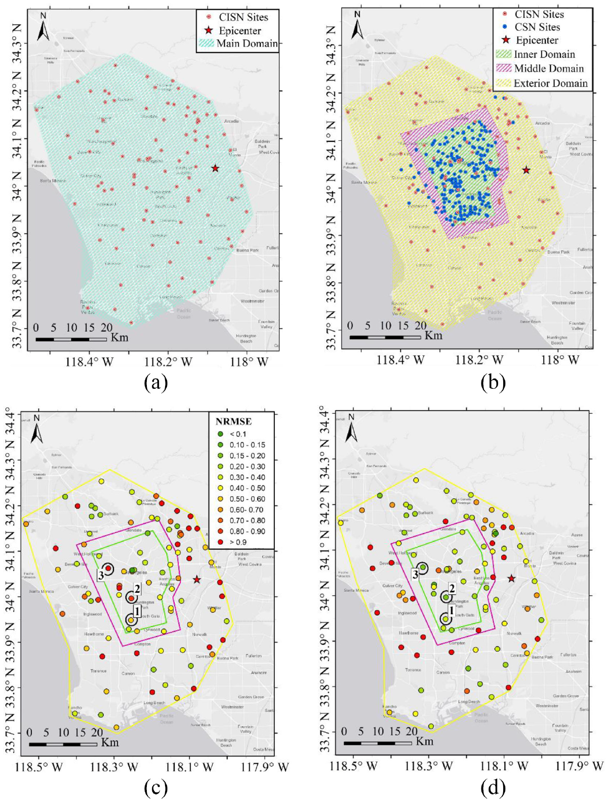
We selected 121 ground-level sites from CISN that recorded the 2019 M7.1 Ridgecrest earthquake in Los Angeles. These 121 recording sites are widely dispersed throughout a 3100 km² region the so-called Main domain (see Figure 10a), whereas the 252 CSN’s sites are placed over a smaller 460 km² region. The distribution of the CSN and CISN installations over Los Angeles is shown in Figure 10b. The $\hat{λ}$ depends on the observation density for each target site, as illustrated in Table 1. Thus, we separated the Main domain into three subdomains: (1) Inner, (2) Middle, and (3) Exterior Domains (Figure 10b). There is one observation density when we use just CISN sites as observation. In contrast, the observation density and the required $\hat{λ}$ are different when we integrate observations from CISN and CSN. Table 3 depicts the observation density and corresponding $\hat{λ}$ for each domain. In Table 3, “Target Domain” refers to the region containing the target sites for which $\hat{λ}$ is suggested. It should be noted that observation density for the sites within Inner, Middle, and Exterior target domains is derived by dividing the number of sites available inside Inner, Inner plus Middle, and Main domains by their respective areas. Although the observation density for the Inner and Middle domains is approximately uniform, the Exterior domain’s density varies from one region to another, similar to the most existing seismic networks. The aforementioned estimate of the overall observation density for the Exterior target region is a suggested approximation by authors to use corresponding $\hat{λ}$ given in Table 1.

Figure 10.

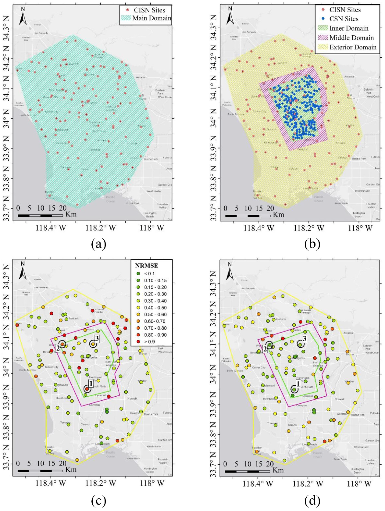
Distribution of (a) CISN sites, (b) CISN and CSN sites, (c) RotD50 spectrum NRMSE for having CISN sites as observation, and (d) RotD50 spectrum NRMSE for having both CISN and CSN sites as observation for 2019 M7.1 Ridgecrest earthquake.

Table 3.

The implemented $\hat{λ}$ for 2019 M7.1 Ridgecrest earthquake

Observations	Target domain	Area (km²)	Observation density (site/km²)	$\hat{λ}$
CISN and CSN	Inner	464	0.57	0.05
CISN and CSN	Middle	764	0.36	0.10
CISN and CSN	Exterior	3103	0.12	0.20
CISN	Main	3103	0.04	0.40

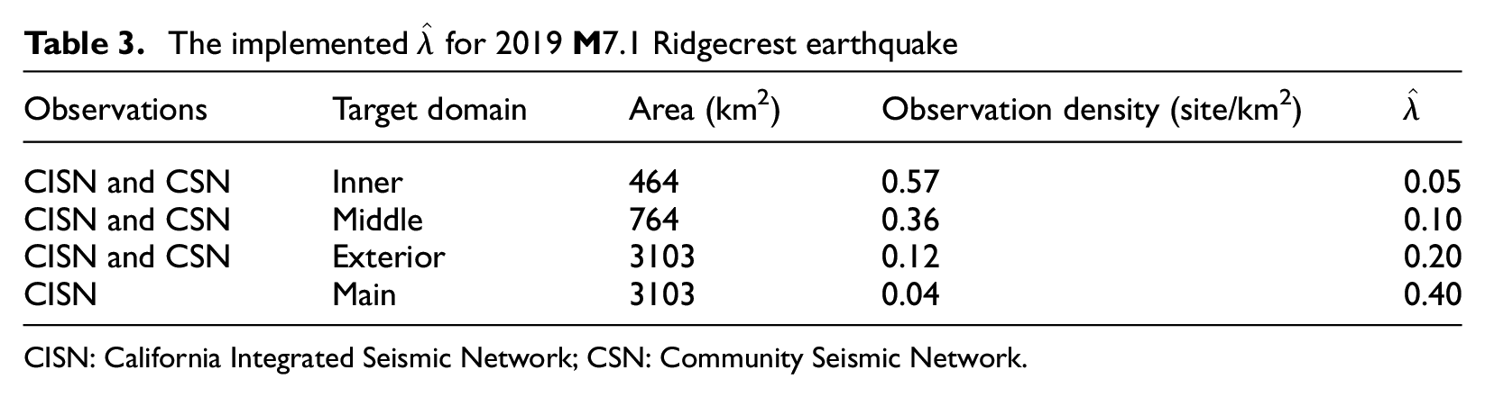
CISN: California Integrated Seismic Network; CSN: Community Seismic Network.

Table 3 demonstrates how the sites within the Exterior domain (Figure 10b) require $\hat{λ} = 0.2$ for having more observations (CISN and CSN). In contrast, the same sites with fewer observations (Figure 10a) need a larger $\hat{λ} = 0.4$ . In addition, it is shown that the inner region of the CISN where the added CSN sites exist requires the smallest $\hat{λ} = 0.05$ .

We need to make the recorded ground motions at the CSN and CISN sites consistent with each other. First, all CISN and CSN motions are rotated to line up with the EW and NS directions. In addition, zero padding at the records’ beginning and end is implemented to ensure that all motions start and finish at the same Universal Time Coordinated (UTC). Finally, the lowest sampling rate among all recorded motions is chosen as the target site’s generated motion’s sampling rate. Figures 10c and d show the distribution of the mean estimated motions’ RotD50 NRMSE. The average RotD50 NRMSE for all target sites using just CISN as observation and both CISN and CSN as observation is 0.48 and 0.39, respectively. This means that the average RotD50 NRMSE is reduced by 19% due to the added CSN sites. In general, the NRMSE below a judgmental value 0.3 indicates a reasonably precise estimation in terms of both time series and response spectrum. However, an NRMSE larger than 0.4 demonstrates a poor estimation. Interested readers are referred to the Appendix section of Tamhidi et al. (2022a), which contains a variety of instances for predictions’ NRMSE.

About 80% of the target sites inside the inner domain had mean estimated motions’ RotD50 NRMSE lower than 0.34. However, there are two sites within the inner domain with RotD50 NRMSE values of 0.52 and 0.9 (orange and red points in Figure 10d). Figure 10b indicates that the majority of added CSN observations are positioned on almost one side of these two target points, resulting in a non-uniform observation distribution around them, which might lead to an inaccurate ground motion estimations as evidenced by Tamhidi et al. (2021). Table 4 compares the average of the mean estimated ground motions’ NRMSE along each horizontal component and RotD50 spectra for various domains.

Table 4.

The prediction error along EW, NS, and RotD50 response spectra in different domains for the 2019 M7.1 Ridgecrest earthquake data set

Domain	Observations	EW		NS		RotD50
Domain	Observations	Average NRMSE	Error reduction^a (%)	Average NRMSE	Error reduction (%)	Average NRMSE	Error reduction (%)
Inner	CISN and CSN	0.33	43	0.37	35	0.29	42
Inner	CISN	0.58	43	0.57	35	0.50	42
Middle	CISN and CSN	0.56	23	0.50	11	0.47	23
Middle	CISN	0.73	23	0.56	11	0.61	23
Exterior	CISN and CSN	0.45	10	0.46	13	0.41	9
Exterior	CISN	0.50	10	0.53	13	0.45	9

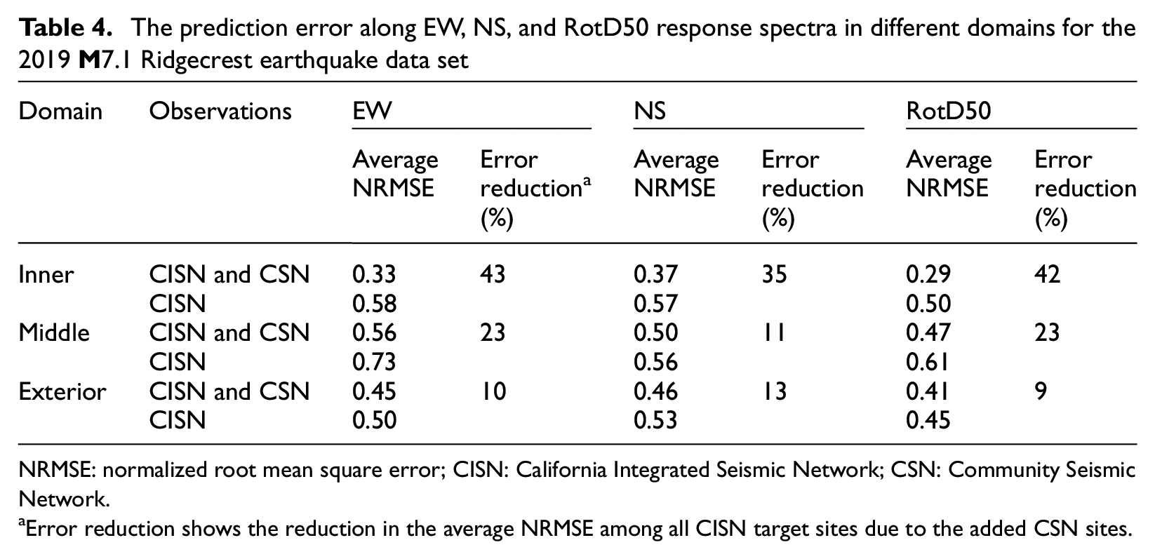
NRMSE: normalized root mean square error; CISN: California Integrated Seismic Network; CSN: Community Seismic Network.

Error reduction shows the reduction in the average NRMSE among all CISN target sites due to the added CSN sites.

Table 4 demonstrates that additional CSN sites generally improve the generated motions’ accuracy along both horizontal components for Inner domain target sites. Furthermore, Table 4 reveals that the added CSN sites had the least impact on the predictions for the target sites in the Exterior domain. Therefore, the prediction for the target sites inside the added network’s borders is improved as more observations become available. However, this effect is less substantial for the target sites outside the added network’s domain. The effect of having more observations on the predictions’ error and uncertainty at different periods is investigated by Tamhidi et al. (2022a).

Three CISN target sites are chosen (Figures 10c and d) to indicate the improvement of the generated motions after adding CSN sites. Figure 11 displays the predicted motions’ RotD50 spectra and velocity time series along EW. Figures 11a and b illustrate how the amplitude of the velocity time series fits closer to the recorded one after observing additional sites from CSN. Similarly, the response spectrum of the prediction matches more precisely to the recorded one, having more observations.

Figure 11.

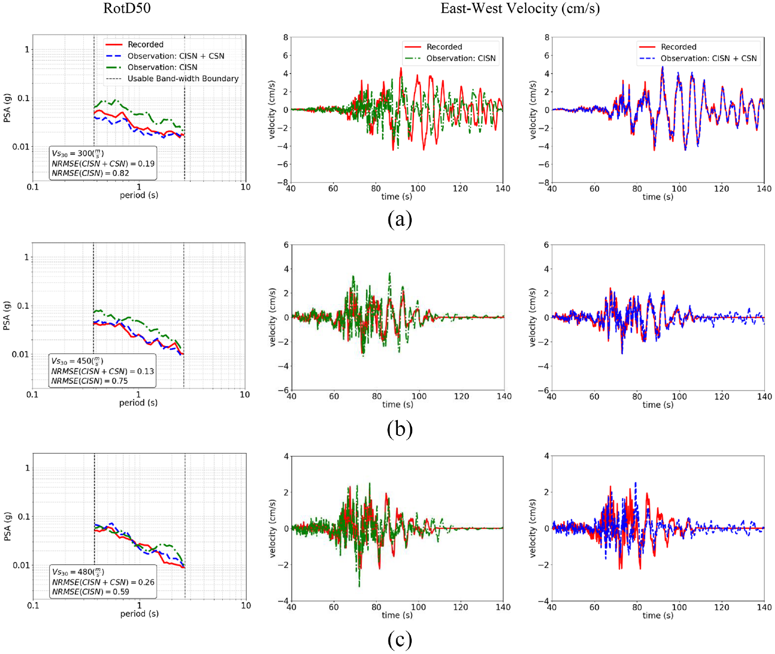
The RotD50 and velocity time series of the prediction using CISN and CISN plus CSN observation along EW direction for the test sites (a) No. 1, (b) No. 2, and (c) No. 3 for 2019 M7.1 Ridgecrest earthquake.

2020 M4.5 South El Monte earthquake

In addition, we evaluate the influence of added observations for the recently recorded ground motions of the 2020 M4.5 South El Monte earthquake. Table 5 outlines the M4.5 South El Monte earthquake characteristics (U.S. Geological Survey (USGS), 2020). We used 95 and 215 ground-level recording sites for CISN and CSN in Los Angeles, respectively (see Figures 12a and b). The number of sites is obtained by eliminating those with a too narrow usable bandwidth.

Figure 12.

Table 5.

The 2020 M4.5 South El Monte earthquake features (USGS, 2020)

Date	UTC time	M_w	Epicenter	Depth
19 September 2020	06:38:46	4.5	South El Monte	16.9 km

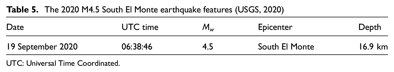
UTC: Universal Time Coordinated.

Table 6 summarizes the observation density and the corresponding employed $\hat{λ}$ . The $\hat{λ}$ for Inner domain having both CISN and CSN sites and $\hat{λ}$ for the Main domain having just CISN sites as observations are obtained using logarithmic interpolation and extrapolation over the $\hat{λ}$ values presented in Table 1, respectively.

Table 6.

The implemented $\hat{λ}$ for 2020 M4.5 South El Monte earthquake

Observations	Target domain	Area (km²)	Observation density (site/km²)	$\hat{λ}$
CISN and CSN	Inner	464	0.46	0.08
CISN and CSN	Middle	764	0.30	0.10
CISN and CSN	Exterior	3103	0.10	0.20
CISN	Main	3103	0.03	0.50

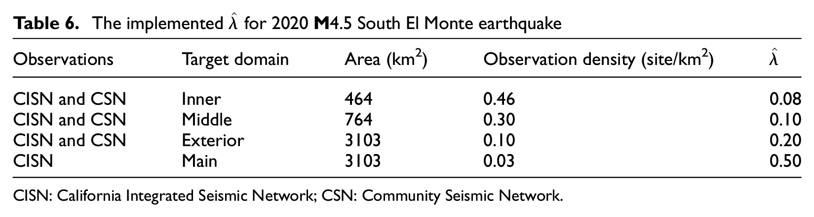
CISN: California Integrated Seismic Network; CSN: Community Seismic Network.

Figures 12c and d demonstrate the distribution of the mean estimated motions’ RotD50 NRMSE at each CISN site. The average RotD50 NRMSE among all target sites for CISN-only and CISN-plus-CSN observed sites is 0.80 and 0.75, respectively. Approximately 67% (12 sites) of the target sites inside the Inner domain had an NRMSE smaller than 0.32 (Figure 12d). There are three target sites inside the Inner domain with an NRMSE larger than 0.5, indicating that their estimates worsened after adding more ground motions from CSN sites.

Table 7 compares the NRMSE of the mean estimated ground motions for each target domain. Table 7 and Figure 12 indicate that the addition of observed sites from CSN, generally improved the prediction of the ground motions inside the Inner domain (30% reduction in RotD50 NRMSE); yet, there are a few sites within the Inner domain where the estimation deteriorated after observing more sites from CSN (orange sites in Figure 12d). Comparing Table 7 and Table 4 reveals that the influence of added CSN sites for the M4.5 South El Monte earthquake is less than that for the M7.1 Ridgecrest earthquake. There are two reasons for the latter. First, the mutual usable bandwidth of the estimated motions for the South El Monte earthquake (0.11–0.55 s) is narrower and shorter than that for the Ridgecrest earthquake (0.38–2.8 s) and it is discussed that the effect of the additional observations on the precision of the generated motions is higher at long periods. Second, the isotropic covariance functions deployed in the GPR model may provide somewhat inaccurate estimates in the epicentral area (Tamhidi et al., 2021). Thus, the added CSN observations might have a negligible effect on improving the estimations for the 2020 M4.5 South El Monte earthquake data set.

Table 7.

The prediction error along EW, NS, and RotD50 response spectra in different domains for the 2020 M4.5 South El Monte earthquake data set

Domain	Observations	EW		NS		RotD50
Domain	Observations	Average NRMSE	Error reduction^a (%)	Average NRMSE	Error reduction (%)	Average NRMSE	Error reduction (%)
Inner	CISN and CSN	0.54	7	0.46	25	0.35	30
Inner	CISN	0.58	7	0.61	25	0.50	30
Middle	CISN and CSN	0.60	−3	0.60	−20	0.50	4
Middle	CISN	0.58	−3	0.50	−20	0.52	4
Exterior	CISN and CSN	0.98	2	1.10	0	0.90	0
Exterior	CISN	1.0	2	1.10	0	0.90	0

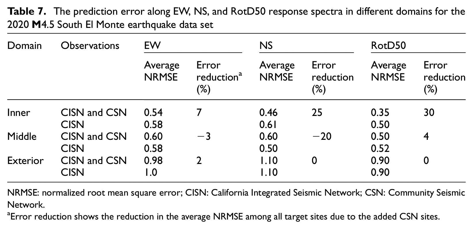
NRMSE: normalized root mean square error; CISN: California Integrated Seismic Network; CSN: Community Seismic Network.

Error reduction shows the reduction in the average NRMSE among all target sites due to the added CSN sites.

The influence of added observations is negligible for the sites within the Middle or Exterior domains and, in some cases, can worsen the estimations. It should be noted that the number of available CISN sites within the Middle domain is sparse (9 sites), which can affect the statistical inference of the added CSN observations’ effect in that region.

Three CISN target sites are selected to demonstrate the estimated ground motion velocity time series using CISN-only, and CISN-plus-CSN observed sites (Figures 12c and d). Figure 13 illustrates the estimated velocity time series along the NS direction using two sets of observations. Figure 13 shows how the velocity time series for the CISN target sites inside the Inner domain fits closer to the recorded one’s amplitude after the GPR model observed more CSN sites.

Figure 13.

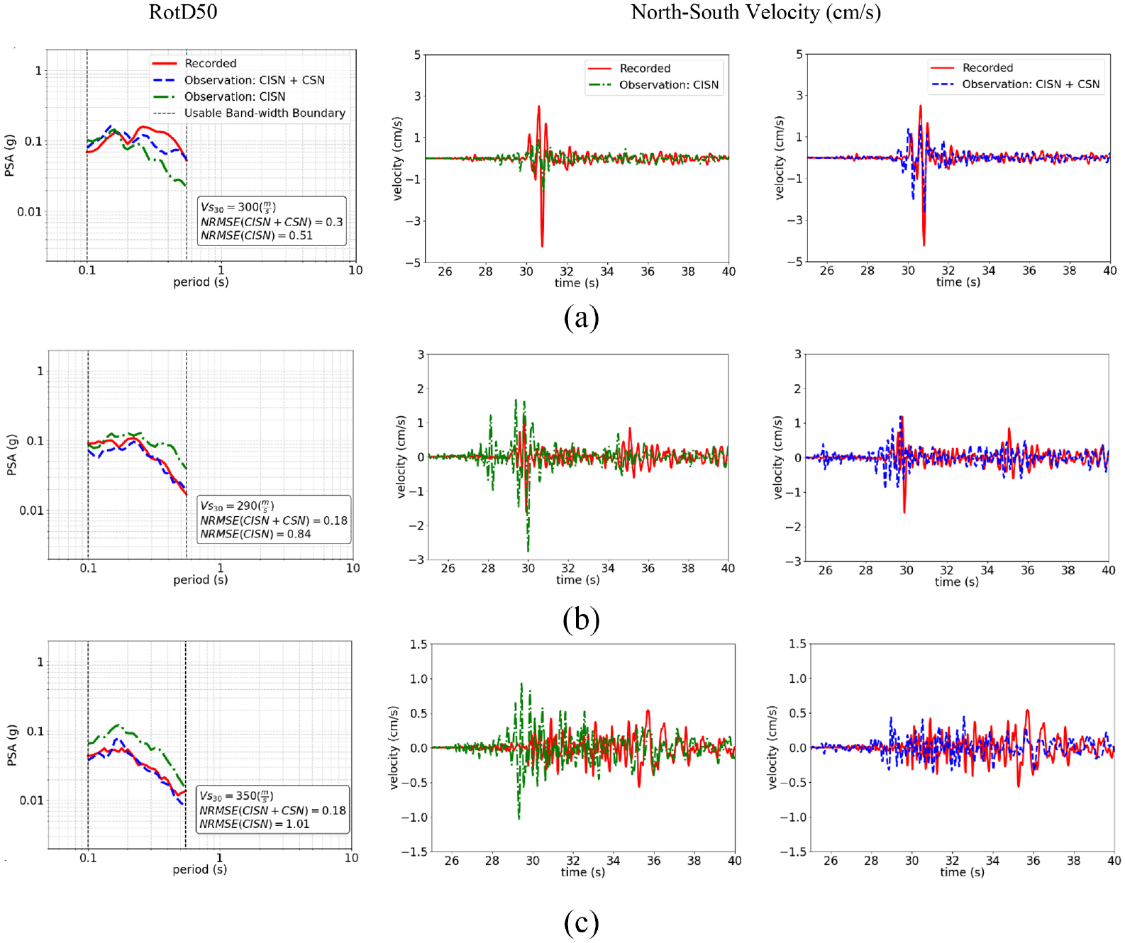
The RotD50 and velocity time series of the prediction using CISN and CISN plus CSN observation along NS direction for the test sites (a) No. 1, (b) No. 2, and (c) No. 3 for 2020 M4.5 South El Monte earthquake.

Concluding remarks

This research aimed to generate post-earthquake ground motion time series at uninstrumented (“target”) sites. We developed a GPR model to generate such ground motions. We explored the influence of observation spatial density (instrumented sites) on the model’s optimal hyperparameter. The optimized hyperparameter allows users to implement the GPR model for various observation densities. It was demonstrated that the required regularization factor is smaller for the region with a higher observation density. In contrast, greater regularization is needed where there are fewer observations.

We also produced ground motion realizations at the target points. This approach offers an ensemble of estimated ground motion time series for uninstrumented sites to conduct the site-specific nonlinear response history analysis, which reveals the uncertainty of the predicted structural damage resulting from record-to-record variation. Quantification of uncertainty of structural responses is a future study which is under development by the authors. The uncertainty of the estimated ground motions is assessed using the generated ground motion realizations at different CSN sites using the 2019 M7.1 Ridgecrest earthquake recorded data set. It is concluded that the number of observed sites closer to the target site plays a vital role in the accuracy and uncertainty of the predictions, particularly at longer periods.

The effect of having additional observations from various recording networks on prediction accuracy was also investigated using the motions recorded during the 2019 M7.1 Ridgecrest and 2020 M4.5 South El Monte earthquakes. As expected, the results demonstrated that the prediction for the target sites located inside the added observed sites’ borders generally improved; yet, there were a few sites with adjacent non-uniform observations that their estimations worsened after observing more ground motions. The influence of additional observations on estimations for the target sites outside the added network’s boundaries was insignificant.

Footnotes

Acknowledgements

The authors thank Prof. Tadahiro Kishida for his efforts in signal processing of the recorded ground motions. Prof. Chukwuebuka Nweke and Prof. Pengfei Wang have kindly provided the estimation of the V_s₃₀, Z_1.0, and Z_2.5 values at the recording stations. Cooperation of Prof. Monica Kohler and Dr Richard Guy on Community Seismic Network (CSN) data is greatly acknowledged. The comments from two Earthquake Spectra anonymous reviewers are appreciated.

Data and Resources

The raw M7.1 2019 Ridgecrest and M4.5 2020 South El Monte earthquakes data recorded by the Community Seismic Network were obtained from https://csn.caltech.edu/data/ (last accessed May 2022). The processed ground motions for the M7.1 2019 Ridgecrest earthquake data set recorded by CSN and CISN can be retrieved from https://www.risksciences.ucla.edu/nhr3/gmdata (last accessed May 2022). The ground motions for the M4.5 2020 South El Monte earthquake recorded by CISN are obtained from the Center for Engineering Strong Motion Data (CESMD) at https://www.strongmotioncenter.org/ (last accessed May 2022). The RotD50 and orthogonal directions linear response spectra of the ground motions were constructed using the R package for computation of earthquake ground motion response spectra (Wang et al., 2017) which is accessible through (last accessed May 2022).

Declaration of conflicting interests

The authors declared no potential conflicts of interest with respect to the research, authorship, and/or publication of this article.

Funding

The authors disclosed receipt of the following financial support for the research, authorship, and/or publication of this article: This study was supported by the University of California, Los Angeles (UCLA) Graduate Fellowship to the first author, which is highly appreciated. Partial support from the National Science Foundation (award no. 2025310), California Department of Transportation, and Pacific Gas and Electric Company is also gratefully acknowledged. Any opinions, findings, conclusions, or recommendations expressed are those of the authors and do not necessarily reflect those of the supporting agencies.

ORCID iDs

Aidin Tamhidi

Nicolas M Kuehn

References

Aagaard

Brocher

Dolenc

Dreger

Graves

Harmsen

Hartzell

Larsen

McCandless

Nilsson

Petersson

(2008) Ground-motion modeling of the 1906 San Francisco earthquake, part II: Ground-motion estimates for the 1906 earthquake and scenario events. Bulletin of the Seismological Society of America 98(2): 1012–1046.

Abrahamson

Schneider

Stepp

(1991) Empirical spatial coherency functions for application to soil-structure interaction analyses. Earthquake Spectra 7(1): 1–27.

Abrahamson

Silva

Kamai

(2014) Summary of the ASK14 ground motion relation for active crustal regions. Earthquake Spectra 30(3): 1025–1055.

Aghababaei

Koliou

Watson

Xiao

(2021) Quantifying post-disaster business recovery through Bayesian methods. Structure and Infrastructure Engineering 17(6): 838–856.

Ahdi

Mazzoni

Kishida

Wang

Nweke

Kuehn

Contreras

Rowshandel

Stewart

Bozorgnia

(2020) Engineering characteristics of ground motions recorded in the 2019 Ridgecrest earthquake sequence. Bulletin of the Seismological Society of America 110(4): 1474–1494.

Alamilla

Esteva

García-Pérez

Díaz-López

(2001) Simulating earthquake ground motion at a site, for given intensity and uncertain source location. Journal of Seismology 5(4): 475–485.

Ancheta

Darragh

Stewart

Seyhan

Silva

Chiou

BSJ

Wooddell

Graves

Kottke

Boore

Kishida

(2014) NGA-West2 database. Earthquake Spectra 30(3): 989–1005.

Atkinson

Assatourians

(2015) Implementation and validation of EXSIM (a stochastic finite-fault ground-motion simulation algorithm) on the SCEC broadband platform. Seismological Research Letters 86(1): 48–60.

Bayless

Abrahamson

(2019) An empirical model for the interfrequency correlation of epsilon for Fourier amplitude spectra. Bulletin of the Seismological Society of America 109(3): 1058–1070.

10.

Boore

(2010) Orientation-independent, nongeometric-mean measures of seismic intensity from two horizontal components of motion. Bulletin of the Seismological Society of America 100(4): 1830–1835.

11.

Boore

Stewart

Seyhan

Atkinson

(2014) NGA-West2 equations for predicting PGA, PGV, and 5% damped PSA for shallow crustal earthquakes. Earthquake Spectra 30(3): 1057–1085.

12.

Campbell

Bozorgnia

(2014) NGA-West2 ground motion model for the average horizontal components of PGA, PGV, and 5% damped linear acceleration response spectra. Earthquake Spectra 30(3): 1087–1115.

13.

Clayton

Kohler

Guy

Bunn

Heaton

Chandy

(2020) CSN-LAUSD network: A dense accelerometer network in Los Angeles Schools. Seismological Research Letters 91(2A): 622–630.

14.

Cui

Hong

(2020) Conditional simulation of spatially varying multicomponent nonstationary ground motions: Bias and ill condition. Journal of Engineering Mechanics 146(2): 04019129.

15.

Deodatis

(1996) Non-stationary stochastic vector processes: Seismic ground motion applications. Probabilistic Engineering Mechanics 11(3): 149–167.

16.

Fraser

Wald

Lin

(2008) Using shakemap and shakecast to prioritize post-earthquake dam inspections. In Manzari

Hiltunen

(eds) Geotechnical Earthquake Engineering and Soil Dynamics IV. Reston, VA: American Society of Civil Engineers, pp. 1–10.

17.

Heredia- Zavoni

Santa-Cruz

(2000) Conditional simulation of a class of nonstationary space-time random fields. Journal of Engineering Mechanics 126(4): 398–404.

18.

Zheng

(2012) Conditional simulation of spatially variable seismic ground motions based on evolutionary spectra. Earthquake Engineering & Structural Dynamics 41(15): 2125–2139.

19.

Kameda

Morikawa

(1992) An interpolating stochastic process for simulation of conditional random fields. Probabilistic Engineering Mechanics 7(4): 243–254.

20.

Kohler

Filippitzis

Heaton

Clayton

Guy

Bunn

Chandy

(2020) 2019 Ridgecrest earthquake reveals areas of Los Angeles that amplify shaking of high-rises. Seismological Society of America 91(6): 3370–3380.

21.

Konakli

Der Kiureghian

(2012) Simulation of spatially varying ground motions including incoherence, wave-passage and differential site-response effects. Earthquake Engineering & Structural Dynamics 41(3): 495–513.

22.

Sudjianto

(2005) Analysis of computer experiments using penalized likelihood in Gaussian Kriging models. Technometrics 47(2): 111–120.

23.

Lin

Wald

Kircher

Slosky

Jaiswal

Luco

(2018) USGS shakecast system advancements. In 11th National Conference on Earthquake Engineering, 2018 June, EERI pp. 3458–3468.

24.

Loos

Lallemant

Baker

McCaughey

Yun

Budhathoki

Khan

Singh

(2020) G-DIF: A geospatial data integration framework to rapidly estimate post-earthquake damage. Earthquake Spectra 36(4): 1695–1718.

25.

Mangalathu

Jeon

(2020) Ground motion-dependent rapid damage assessment of structures based on wavelet transform and image analysis techniques. Journal of Structural Engineering 146(11): 04020230.

26.

Nweke

Wang

Brandenberg

Stewart

(2018) Reconsidering basin effects in ergodic site response models. UCLA. Retrieved from https://escholarship.org/uc/item/6048v74k

27.

Oppenheim

Willsky

Nawab

(1997) Signals and Systems. Prentice hall Inc., Upper Saddle River, NJ.

28.

Rasmussen

Williams

CKI

(2006) Gaussian Processes for Machine Learning. Cambridge, MA: The MIT Press.

29.

Rodda

Basu

(2018) Coherency model for translational and rotational ground motions. Bulletin of Earthquake Engineering 16(7): 2687–2710.

30.

Rodgers

Anders Petersson

Pitarka

McCallen

Sjogreen

Abrahamson

(2019) Broadband (0–5 Hz) fully deterministic 3D ground-motion simulations of a magnitude 7.0 Hayward fault earthquake: Comparison with empirical ground-motion models and 3D path and site effects from source normalized intensities. Seismological Research Letters 90(3): 1268–1284.

31.

Roohi

Hernandez

(2020) Performance-based post-earthquake decision making for instrumented buildings. Journal of Civil Structural Health Monitoring 10(5): 775–792.

32.

Shinozuka

Deodatis

(1996) Simulation of multi-dimensional Gaussian stochastic fields by spectral representation. Appl Mech Rev 49 (1): 29–53. https://doi.org/10.1115/1.3101883

33.

Southern California Earthquake Data Center (2022) Available at: https://service.scedc.caltech.edu/SCSNStationMap/station.html (accessed May 2022).

34.

Tamhidi

Kuehn

Bozorgnia

(2022a) Uncertainty and Sensitivity Analysis of Conditioned Simulation of Ground Motion using Gaussian Process Regression. University of California, Los Angeles. Natural Hazards Risk & Resiliency Research Center. DOI: 10.34948/N39G6W.

35.

Tamhidi

Kuehn

Ghahari

Rodgers

Kohler

Taciroglu

Bozorgnia

(2021) Conditioned simulation of ground-motion time series at uninstrumented sites using Gaussian process regression. Bulletin of the Seismological Society of America 112(1): 331–347. DOI: 10.1785/0120210054.

36.

Tamhidi

Kuehn

Ghahari

Rodgers

Taciroglu

Bozorgnia

, (2022b) Earthquake ground motion conditioned simulation using sparsely distributed observed motions for analysis and design of lifeline structures. Proceedings of Lifelines 2022 Conference, Los Angeles, CA, February, Reston, VA: American Society of Civil Engineers.

37.

Tamhidi

Kuehn

Kohler

Ghahari

Taciroglu

Bozorgnia

(2020) Ground-motion time-series interpolation within the community seismic network using Gaussian process regression: Application to the 2019 Ridgecrest earthquake. In Poster Presentation at 2020 SCEC Annual Meeting, September 2020.

38.

Thomson

Bradley

Lee

(2020) Methodology and computational implementation of a New Zealand Velocity Model (NZVM2. 0) for broadband ground motion simulation. New Zealand Journal of Geology and Geophysics 63(1): 110–127.

39.

U.S. Geological Survey (2020). M4.5-3km WSW of South El Monte, CA. Available at: https://earthquake.usgs.gov/earthquakes/eventpage/ci38695658/executive (accessed May 2022.).

40.

Vanmarcke

Fenton

(1991) Conditioned simulation of local fields of earthquake ground motion. Structural Safety 10(1–3): 247–264.

41.

Vehtari

Gelman

Gabry

(2017) Practical Bayesian model evaluation using leave-one-out cross-validation and WAIC. Statistics and Computing 27(5): 1413–1432.

42.

Wald

Lin

Porter

Turner

(2008) ShakeCast: Automating and improving the use of ShakeMap for post-earthquake decision-making and response. Earthquake Spectra 24(2): 533–553.

43.

Wang

Stewart

Bozorgnia

Boore

Kishida

(2017) R package for computation of earthquake ground motion response spectra. Pacific Earthquake Engineering Center, Report 2017/09.

44.

Weatherill

Silva

Crowley

Bazzurro

(2015) Exploring the impact of spatial correlations and uncertainties for portfolio analysis in probabilistic seismic loss estimation. Bulletin of Earthquake Engineering 13(4): 957–981.

45.

Wen

Ellingwood

Veneziano

Bracci

. (January, 2003) Uncertainty modeling in earthquake engineering. Mid-America Earthquake Center Project FD-2 report

46.

Worden

Thompson

Baker

Bradley

Luco

Wald

(2018) Spatial and spectral interpolation of ground-motion intensity measure observations. Bulletin of the Seismological Society of America 108(2): 866–875.

47.

Gao

(2015) Error assessment of multivariate random processes simulated by a conditional-simulation method. Journal of Engineering Mechanics 141(5): 04014155.

48.

Yazdi

Motamed

Anderson

(2022) A new set of automated methodologies for estimating site fundamental frequency and its uncertainty using horizontal-to-vertical spectral ratio curves. Seismological Society of America 93(3): 1721–1736.

49.

Zentner

(2013) Simulation of non-stationary conditional ground motion fields in the time domain. Georisk: Assessment and Management of Risk for Engineered Systems and Geohazards 7(1): 37–48.

Uncertainty quantification of ground motion time series generated at uninstrumented sites

Abstract

Keywords

Introduction

Theoretical background

Gaussian Process Regression

Hyperparameter optimization

Ground motion random realizations

Uncertainty quantification and sensitivity analysis

Performance evaluation on combined network data sets

2019 M7.1 Ridgecrest earthquake

2020 M4.5 South El Monte earthquake

Concluding remarks

Footnotes

Acknowledgements

Data and Resources

Declaration of conflicting interests

Funding

ORCID iDs

References