Sage Journals: Discover world-class research

Abstract

In this study, a simplified shallow three-dimensional shear wave velocity (Vs) model is presented for the Mexico City Basin. To this end, previous studies were carefully reviewed to assemble a database of Vs and site period measurements for the region. The new site period measurements obtained at the western edge of the Basin were compared to the existing 2004 Complementary Technical Standards of Mexico site period nominal map, (NTC, 2004) the Lermo et al. (2020) site period map, and Design Seismic Actions System (SASID), 2020 site period predictions. Each site period prediction method was shown to have differences with respect to the new measurements along the western edge of the Basin. However, there was no bias for the prediction methods with the Lermo et al. (2020) and SASID predictions, demonstrating less error between the measured values than the NTC (2004) predictions. To develop the three-dimensional Vs model, the shallow (top 60 m) subsurface was divided into five generalized soil layers. The site period was used as the only input for the three-dimensional Vs model to simplify and maximize the model’s applicability. The performance of the model was assessed by comparing the measured and predicted Vs profiles. Overall, the three-dimensional Vs model developed in this study is a valuable tool that can be used along with geophysical estimates of deeper structure for ground motion modeling and preliminary site response studies along with other benefits to the seismic resiliency of the region.

Keywords

Mexico City shear wave velocity three-dimensional model site period earthquake engineering

Introduction

The unique geologic setting of the Mexico City Basin (Figure 1) (Mooser, 1990) and its extraordinary seismic response (Aki, 1988; Bard and Bouchon, 1980a, 1980b; Campillo et al., 1989; Kawase and Aki, 1989; Ordaz and Singh, 1992; Sánchez-Sesma et al., 1988; Singh et al., 1988) highlights the need for a comprehensive understanding of the seismic properties of the subsurface layers across the basin. Its complex formation has been the result of several geological processes that have occurred in the region, such as the high volcanic and tectonic activity. At the edge of the basin, the shallow portions of the geological sequence are comprised of Pliocene-Pleistocene to recent Holocene volcanic rocks, like andesite and dacite, forming series of mountain ranges around the basin (i.e. Sierra de Guadalupe, Sierra de las Cruces, Sierra Nevada, Sierra Ajusco, and Sierra de Chichinautzin). Further inside descending from the volcanic ranges, there is a series of pyroclastic flows comprised of breccias and tuffs, locally known as “Tarango formation,” followed by alluvium deposits that extend throughout the Basin’s edges. Finally, there are the lacustrine deposits of soft clay formed by the sedimentation of volcanic ash and other pyroclastic materials on the old lakes, which were created after the closure of the Basin by basaltic lava flows during the Quaternary (Arce et al., 2019; Mooser, 1990). Figure 1a shows the general perspective of the geological complex configuration of the Basin, where it can appreciate the distribution of the sequence described above, and Figure 1b depicts the typical stratigraphy of the lake zone. Within the last 50 years, Mexico City has experienced four major seismic events, with the 2017 Mw 7.1 Puebla-Morelos Earthquake as one of the most recent destructive earthquakes (Geotechnical Extreme Events Reconnaissance [GEER], 2020). These earthquakes led to severe damage to the buildings and infrastructure due to the complex and variable subsurface layering (particularly the very soft unconsolidated lacustrine clay layer) and hydrological settings of this area (Mayoral et al., 2019; Pestana et al., 2002; Seed et al., 1988). As the population and infrastructure continue to rapidly expand in the region, it is mandatory that the understanding of the seismic site response of the region advances as well. Consequently, the shear wave velocity (Vs) and the fundamental site period are of particular interest in seismic design as these impact the seismic site response, and the Basin’s significant generation of surface waves (Baena-Rivera, 2017; Baena-Rivera et al., 2023; Chávez-García and Salazar, 2002; Pérez-Rocha et al., 1995; Sánchez-Sesma et al., 1993a). The ability to assess these properties across the Basin and compute the seismic response are essential elements for accurate seismic design.

Figure 1.

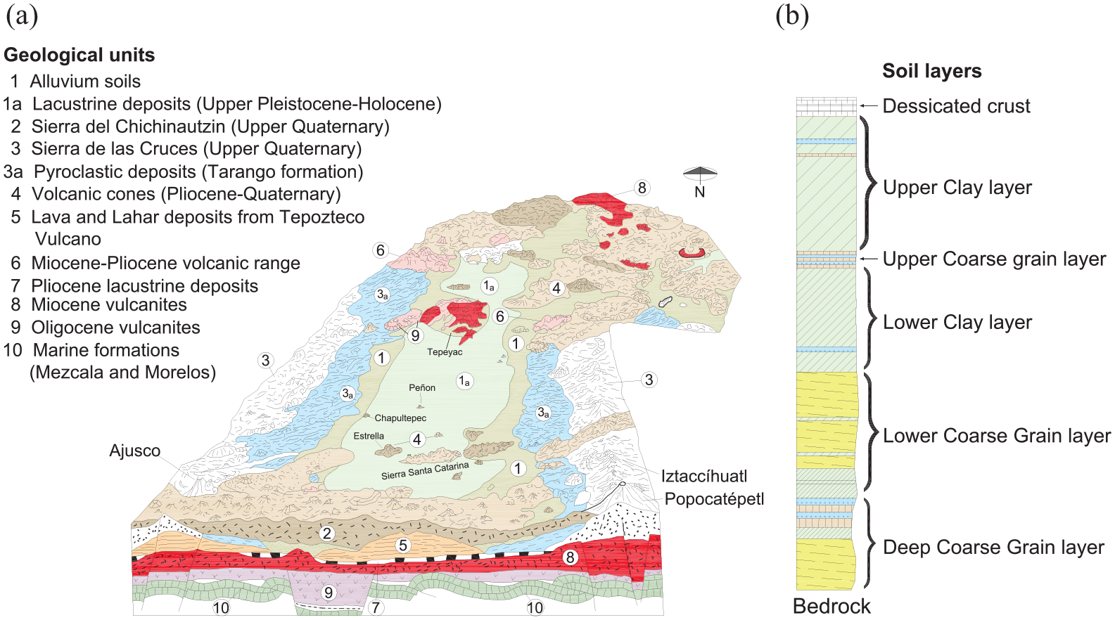
(a) Geology and morphology of the Mexico City Basin and (b) typical soil profile at lake zone (Zone III) (modified from Santoyo et al., 2005).

Measuring the fundamental site period of a particular site is indispensable in the design of seismic resilient structures. During a seismic event, composed of a broad range of frequencies, the seismic loading on the building will be significantly increased if the fundamental site period of the soil is close to the resonant period of the structure. This phenomenon was present in damage observed on the western edge of the Mexico City Basin during the 2017 Mw 7.1 Puebla-Morelos Earthquake (Franke et al., 2019). Various site period maps exist for Mexico City. The Mexican Seismic Design Code (NTC, 2004) site period map has been often used to obtain site period estimates across the Basin. These site periods are related to engineering bedrock around the edge of the Basin with nominal periods less than 0.5 s, but they are related to a stiff sediment layer within the interior of the Basin. However, studies have shown that the site period in the lacustrine clay zone is changing due to consolidation from groundwater extraction (Arroyo et al., 2013; Wood et al., 2019). This further complicates and undermines the ability of engineers to design a seismically resilient structure and highlights the need for updating continuously the current site period map. To this end, Lermo et al. (2020) published an updated site period map of the Basin to improve the accuracy of site period estimates within the areas of the Basin which are changing.

Another important dynamic soil property is the shear wave velocity (Vs) of the subsurface materials. The Vs is used for several purposes in seismic design, such as the determination of seismic site class (e.g. Rahimi et al., 2020a), natural site period estimation (e.g. Wang et al., 2018), wave propagation modeling (e.g. Cruz-Atienza et al., 2016; Nishizawa et al., 1997), site effects estimates (e.g. Anbazhagan and Sitharam, 2020), and liquefaction analysis (e.g. Rahimi et al., 2020b). Moreover, the Vs profile and its spatial variation controls the emergence of surface waves (e.g. Chávez-García and Salazar, 2002; Molina-Villegas et al., 2018; Sánchez-Sesma et al., 1993b). For the Mexico City Basin, the Vs profile changes significantly across the Basin (Wood et al., 2023). This is of particular interest for the very soft lacustrine clay layer, which is one of the critical factors controlling site effects in the Basin. Moreover, the seismic properties of the lacustrine clay layer change over time due to consolidation of the clay layer. This adds more ambiguity and complexity in predicting the Vs profile at sites across the Basin. Several studies have gathered Vs data for specific sites within the Basin (e.g. Mayoral et al., 2008, 2016; Wood et al., 2019), but currently, no Vs prediction model exists in the region for shallow near-surface deposits (top 30–60 m). Therefore, the ability to model the Vs throughout the Basin would bring numerous benefits to the seismic resiliency of the region. However, the seismic response on this complex seismic environment is a consequence of amplification provided by the 1D response (Chávez-García, 2010; Chávez-García and Bard, 1994; Kawase and Aki, 1989; Seed et al., 1988), locally generated surface waves, and three-dimensional obliquely incident body waves. Fortunately, these physical considerations are accounted for in the current crafting of the design spectra. Moreover, the three-dimensional (3D) Vs model can be the input of physics-based advanced simulations of seismic response (e.g. Hernández-Aguirre et al., 2023).

The main goals of this study are (1) assess the accuracy of both the NTC (2004) and Lermo et al. (2020) site period maps, and (2) develop a simplified shallow 3D Vs model for the Mexico City Basin. This article builds upon the work in Wood et al. (2023), which presents site period and shear wave velocity measurements made in the Mexico City Basin and provides initial analysis of trends in the data and areas of agreement and disagreement within the data set. Therefore, in this article, previous studies are carefully reviewed to build a larger data set of site period and Vs measurements in the Basin beyond the Wood et al. (2023) data set. The data selection for developing the site period and Vs data sets is first discussed. The final sites and data used in this study to assess the site period maps and develop the 3D Vs model are then provided. This is followed by the Results and Discussions sections, where the data variability and trends are first examined. An assessment of the site period maps, and the 3D Vs model are then detailed. Finally, some conclusions are provided regarding the site period maps and the 3D Vs model. We are currently engaged in incorporating more sites and data to have a more robust model and to continue updating the 3D model presented in this study; these matters are currently being addressed and will be considered for future publications.

Data selection

The first step toward developing a 3D shear wave velocity model and assessing the site period map from NTC (2004) and Lermo et al. (2020) is to build a Vs and site period data set for the Mexico City Basin. In this regard, all available site-specific data for Vs and site period from the literature were carefully reviewed and compiled. These data were then filtered based on how well their natural site periods and/or Vs profiles matched nearby sites and whether the measurements met the requirements of the model (i.e. represented shallow Vs information). This step was taken to initially remove the influence of outliers in the preliminary steps of creating the 3D Vs model. At the end of this process, 75 sites were selected to assess the site period map and 40 sites were selected to develop the 3D Vs model. The distribution of the selected sites per each seismic zone defined in NTC (2004) is tabulated in Table 1; most of the sites are located in Zones II, IIIa, and IIIb.

Table 1.

Distribution of sites for each Normas Técnicas Complementarias (NTC) 2004 seismic zone

Zone	Number of sites for revised site period map	Number of sites for Vs model
I	1	2
II	16	9
IIIa	18	14
IIIb	22	12
IIIc	9	1
IIId	9	2

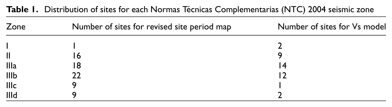
Figure 2 shows the distribution of the sites used in the present study for the 3D Vs model along with the defined seismic zones from NTC (2004). Included in the figure are sites where earthquake horizontal-to-vertical spectral ratio (EHVSR), microtremor horizontal-to-vertical spectral ratio (MHVSR), and shear wave velocity (Vs) measurements were made. From Figure 2, most sites included in this study are located along the Basin’s western edge. This is because most of the data used in this study are related to the investigations conducted following the Mw 7.1 on 19 September 2017 Puebla-Morelos earthquake. These investigations were mainly concentrated on the western edge of the Basin because the majority of the severely building damages were observed in these areas (Franke et al., 2019). Detailed information regarding this damage was provided in the GEER (2020) and Franke et al. (2019).

Figure 2.

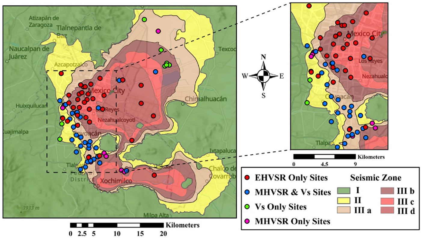
Sites used in this study organized by data category along with the NTC (2004) site period zonation map.

Data used for site period map evaluation

The NTC (2004) site period zonation map was the most used map for site period prediction across the Basin previous to and shortly after the 2017 earthquake. This map provided the best estimate of the site period across the Basin (Wood et al., 2019). However, Lermo et al. (2020) published a new site period map which benefited from additional measurements across the Basin. In addition, the Design Seismic Actions System (Sistema de Acciones Sísmicas de Diseño (SASID), 2020), an online computer system which is the interface between users and the regulatory guidelines, provides site period information across parts of the Mexico City Basin. However, it does not have an associated site period map and only provides discrete values of site period. The site period data used herein comes from previous investigations which are independent from any current site period map and includes both EHVSR and MHVSR measurements. These data come primarily from Hayashi et al. (2011), Wood et al. (2019), and Wood et al. (2023). A total of 34 EHVSR and 41 MHVSR measurements were used, which are the 75 sites mentioned in Table 1 and shown in Figures 1 and 2. The final data set used to evaluate the site period maps from the EHVSR and MHVSR are tabulated in Tables 2 and 3, respectively. Information provided in these tables includes the site name, coordinates, the measured site period, the associated seismic Zone from NTC (2004), the collector, and the discrete SASID (2020) predicted site period at each location.

Table 2.

Earthquake horizontal to vertical spectral ratio, EHVSR, sites used in the study

Site	Latitude (°)	Longitude (°)	Siteperiod (s)	Zone	Collector	Site period (s)obtained fromSASID
AL01	19.43560	−99.14530	1.92	IIIb	Wood et al. (2019)	1.9
AU46	19.38320	−99.16810	1.05	II	Wood et al. (2019)	0.8
BA49	19.40970	−99.14500	2.33	IIIc	Wood et al. (2019)	2.4
BL45	19.42530	−99.14810	1.72	IIIb	Wood et al. (2019)	2.1
BO93	19.46620	−99.10506	2.93	IIIc	Wood et al. (2019)	2.4
CA59	19.42677	−99.11884	2.56	IIIc	Wood et al. (2019)	2.7
CCCL	19.44980	−99.13700	1.85	IIIb	Wood et al. (2019)	1.8
CE23	19.46296	−99.06103	4.34	IIId	Wood et al. (2019)	4.6
CI05	19.41860	−99.16530	1.39	IIIb	Wood et al. (2019)	2.0
CJ04	19.40970	−99.15670	1.79	IIIb	Wood et al. (2019)	1.9
DM12	19.43328	−99.09724	3.00	IIId	Wood et al. (2019)	3.1
EO30	19.38850	−99.17720	0.61	II	Wood et al. (2019)	0.6
GA62	19.43850	−99.14010	2.04	IIIb	Wood et al. (2019)	1.9
GC38	19.31610	−99.10590	1.72	IIIb	Wood et al. (2019)	1.6
GR27	19.47556	−99.18015	1.00	II	Wood et al. (2019)	0.8
HJ72	19.42510	−99.13010	2.22	IIIc	Wood et al. (2019)	2.3
JA43	19.40637	−99.12574	2.38	IIIc	Wood et al. (2019)	2.9
JC54	19.31300	−99.12720	1.20	IIIa	Wood et al. (2019)	1.1
MY19	19.34610	−99.04330	2.78	IIIc	Wood et al. (2019)	2.7
N/A	19.45284	−99.02545	4.00	IIId	Wood et al. (2019)	No data
NZ20	19.39341	−99.00161	4.00	IIId	Wood et al. (2019)	No data
NZ31	19.41780	−99.02533	5.10	IIId	Wood et al. (2019)	No data
PD42	19.40636	−99.10003	4.00	IIId	Wood et al. (2019)	3.8
PE10	19.39028	−99.13239	2.00	IIIb	Wood et al. (2019)	2.0
RM48	19.43590	−99.12800	2.13	IIIb	Wood et al. (2019)	2.3
SCT	19.39470	−99.14870	1.69	IIIb	Wood et al. (2019)	1.8
SI53	19.37530	−99.14830	1.43	IIIa	Wood et al. (2019)	1.4
TH35	19.27860	−99.00000	3.80	IIId	Wood et al. (2019)	4.7
TL08	19.45000	−99.13360	1.72	IIIb	Wood et al. (2019)	1.9
TL55	19.45360	−99.14250	1.75	IIIb	Wood et al. (2019)	1.4
UC44	19.43370	−99.16540	1.45	IIIa	Wood et al. (2019)	1.3
VC09	19.45478	−99.12277	2.10	IIIb	Wood et al. (2019)	2.1
VM25	19.38154	−99.12531	2.27	IIIc	Wood et al. (2019)	2.3
XP04	19.41980	−99.13530	2.33	IIIc	Wood et al. (2019)	2.3

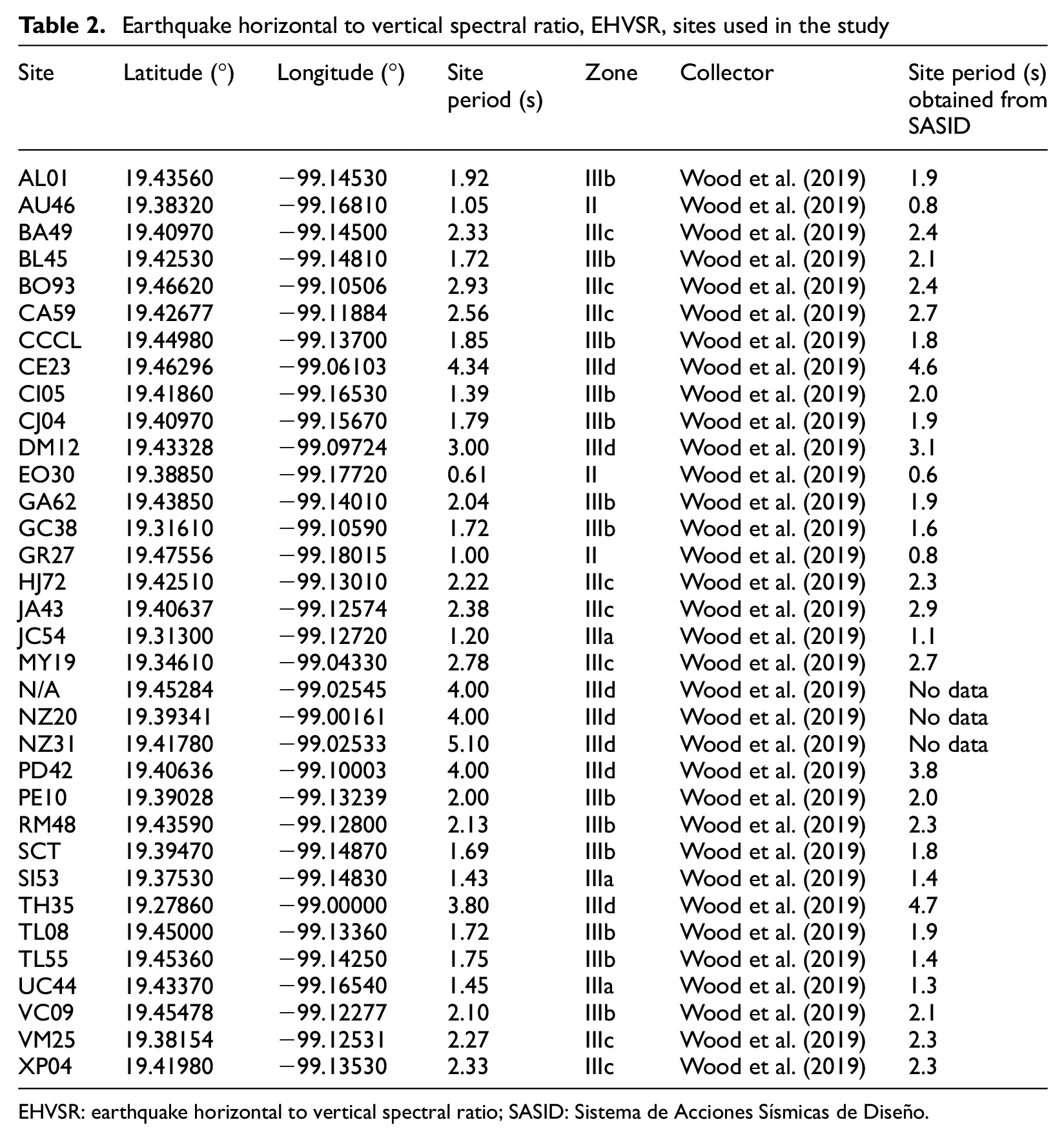
EHVSR: earthquake horizontal to vertical spectral ratio; SASID: Sistema de Acciones Sísmicas de Diseño.

Table 3.

Microtremor horizontal to vertical spectral ratio, MHVSR, sites used in the study

Site	Latitude (°)	Longitude (°)	Site period (s)	Zone	Collector	Site period (s)obtained from SASID
Bosque Aragon	19.46228	−99.06756	3.90	IIId	Hayashi et al. (2011)	4.2
Av Sirena	19.28510	−99.05783	1.67	IIIb	Wood et al. (2019)	1.7
Chapultepec	19.42294	−99.18256	0.70	II	Hayashi et al. (2011)	0.7
Del Mar Tlahuac	19.28838	−99.06356	2.00	IIIb	Wood et al. (2019)	1.4
Escocia Del Valle	19.38744	−99.16342	0.93	II	Wood et al. (2019)	1.0
H/V 1, Condesa	19.41456	−99.17408	1.09	II	Wood et al. (2019)	1.1
H/V 2, Condesa	19.41294	−99.17477	1.04	II	Wood et al. (2019)	1.1
H/V 3, Condesa	19.41148	−99.17576	0.94	II	Wood et al. (2019)	1.0
H/V 4, Hipódromo Condesa	19.40897	−99.17729	0.91	II	Wood et al. (2019)	0.9
Hospital Gral Tlahuac	19.28735	−99.05354	2.00	IIIb	Wood et al. (2019)	1.6
La Morena	19.39861	−99.15873	1.28	IIIa	Wood et al. (2019)	1.4
Parque España	19.41546	−99.17138	1.35	IIIa	Wood et al. (2019)	1.3
Paseo las Galias	19.32139	−99.09711	1.09	II	Wood et al. (2019)	1.2
Rancho Los Arcos	19.30449	−99.12294	1.00	IIIa	Wood et al. (2019)	1.0
Lomas Estrella	19.31511	−99.09303	1.63	IIIb	Wood et al. (2019)	1.3
Parque Floresta (Site 1)	19.30445	−99.12917	0.89	IIIa	Wood et al. (2023)	0.9
Parque La Fuente (Site 2)	19.29454	−99.13322	0.94	IIIa	Wood et al. (2023)	0.9
Parque Campestre (Site 3)	19.30957	−99.11674	1.27	IIIa	Wood et al. (2023)	1.1
San Francisco Culhuacan (Site 4)	19.33081	−99.12665	1.25	IIIa	Wood et al. (2023)	1.3
Parque Xotepingo (Site 5)	19.33493	−99.14232	0.93	IIIa	Wood et al. (2023)	1.0
Parque Mashai (Site 6)	19.34186	−99.13422	1.09	IIIa	Wood et al. (2023)	1.1
Parque Masayoshi Ohira (Site 7)	19.35220	−99.14198	0.99	IIIa	Wood et al. (2023)	1.1
Hacienda Vista Hermosa (Site 8)	19.30234	−99.10560	2.08	IIIb	Wood et al. (2023)	2.2
Parque El Triangulo (Site 9)	19.31441	−99.10928	1.59	IIIa	Wood et al. (2023)	1.3
Parque Salvador Allende (Site 10)	19.30660	−99.12343	1.30	IIIa	Wood et al. (2023)	1.0
Ejido Tlahuac (Site 11)	19.33679	−99.12641	1.33	IIIa	Wood et al. (2023)	1.1
Parque Naciones Unidas (Site 12)	19.34364	−99.12431	1.32	IIIa	Wood et al. (2023)	1.2
ESIME (Site 13)	19.33145	−99.11256	0.99	II	Wood et al. (2023)	0.7
Parque Italia (Site 14)	19.31407	−99.12635	1.09	IIIa	Wood et al. (2023)	1.1
Hacienda San Juan (Site 15)	19.28992	−99.14285	0.78	II	Wood et al. (2023)	0.6
Parque Huayamilpas (Site 16)	19.32342	−99.15083	0.74	I	Wood et al. (2023)	0.5
Parque Xicoténcatl (Site 18)	19.35633	−99.15094	1.01	II	Wood et al. (2023)	1.1
Parque de la Conchita (Site 19)	19.34706	−99.15934	0.65	II	Wood et al. (2023)	0.7
Parque de los Venados (Site 20)	19.37187	−99.15643	1.09	II	Wood et al. (2023)	1.1
Parque Odesa (Site 21)	19.39115	−99.14328	1.54	IIIb	Wood et al. (2023)	2.0
Mixhuca (Site 23)	19.40897	−99.10816	3.33	IIId	Wood et al. (2023)	3.3
Parque Alfonso Esparza (Site 24)	19.38944	−99.17750	0.55	II	Wood et al. (2023)	0.6
Parque Las Americas (Site 25)	19.40028	−99.14917	1.89	IIIb	Wood et al. (2023)	2.1
Texcoco No. 7	19.47883	−98.99748	3.33	IIIc	Hayashi et al. (2011)	No data
Texcoco No. 8	19.55757	−98.99228	1.13	IIIa	Hayashi et al. (2011)	No data
Texcoco TXC	19.49203	−98.97625	2.30	IIIb	Hayashi et al. (2011)	No data

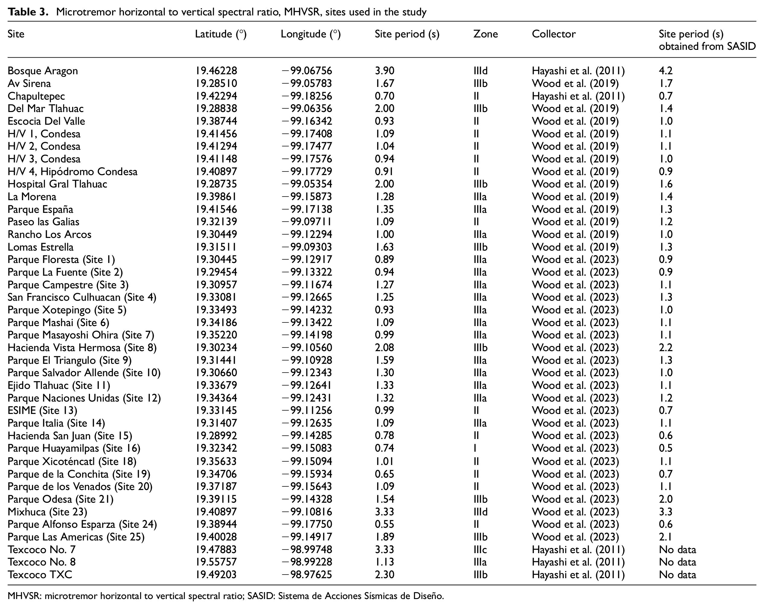
MHVSR: microtremor horizontal to vertical spectral ratio; SASID: Sistema de Acciones Sísmicas de Diseño.

The site periods considered in this study (Tables 2 and 3) are compared with those obtained from (1) the NTC (2004), (2) Lermo et al. (2020) site period maps, and (3) SASID (2020) later in the article. The requirement to use the SASID online interface emerged as an update to the NTC, 2004 requirements, which was motivated by, among other reasons, the damage due to the 2017 earthquake. The label “no data” in Tables 2 and 3 is because these points are located outside Mexico City, and the new regulation only has data within the city.

Data used for the 3D shear wave velocity model

Data used for the 3D shear wave velocity model were extracted from seven different studies, including Díaz-Rodríguez et al. (1998), Stephenson and Lomnitz (2005), Hayashi et al. (2011), Mayoral et al. (2016), O’Riordan et al. (2017), Wood et al. (2019), and Wood et al. (2023). The final 40 sites that were used for the 3D shear wave velocity model are tabulated in Table 4. Information provided in this table includes site name, coordinates, associated seismic Zone from NTC (2004), collector, and the testing method used to generate the 1D Vs profile.

Table 4.

Vs sites used for the 3D Vs model

Site	Latitude (°)	Longitude (°)	Zone	Collector	Testing method
Alameda	19.43585	−99.14497	IIIb	Hayashi et al. (2011)	Surface Wave Testing
Bosque Aragon	19.46228	−99.06756	IIId	Hayashi et al. (2011)	Surface Wave Testing
Chapultepec	19.42294	−99.18256	II	Hayashi et al. (2011)	Surface Wave Testing
Escocia Del Valle	19.38744	−99.16342	II	Wood et al. (2019)	Surface Wave Testing
Hospital Gral Tlahuac	19.28735	−99.05354	IIIb	Wood et al. (2019)	Surface Wave Testing
La Morena	19.39861	−99.15873	IIIa	Wood et al. (2019)	Surface Wave Testing
NAICM	19.52107	98.98670	IIIb	O’Riordan et al. (2017)	Suspension Logging
Parque Espana	19.41546	−99.17138	IIIa	Wood et al. (2019)	Surface Wave Testing
Parque Ramón López-Velarde	19.40000	−99.15000	IIIb	Díaz-Rodríguez et al. (1998)	Crosshole Testing
Parque Floresta (Site 1)	19.30445	−99.12917	IIIa	Wood et al. (2023)	Surface Wave Testing
Parque Salvador Allende (Site 10)	19.30660	−99.12343	IIIa	Wood et al. (2023)	Surface Wave Testing
Ejido Tlahuac (Site 11)	19.33679	−99.12641	IIIa	Wood et al. (2023)	Surface Wave Testing
Parque Naciones Unidas (Site 12)	19.34364	−99.12431	IIIa	Wood et al. (2023)	Surface Wave Testing
ESIME (Site 13)	19.33145	−99.11256	II	Wood et al. (2023)	Surface Wave Testing
Parque Italia (Site 14)	19.31407	−99.12635	IIIa	Wood et al. (2023)	Surface Wave Testing
Hacienda San Juan (Site 15)	19.28992	−99.14285	II	Wood et al. (2023)	Surface Wave Testing
Parque Huayamilpas (Site 16)	19.32342	−99.15083	I	Wood et al. (2023)	Surface Wave Testing
Parque Tagle (Site 17)	19.34824	−99.18268	I	Wood et al. (2023)	Surface Wave Testing
Parque Xicoténcatl (Site 18)	19.35633	−99.15094	II	Wood et al. (2023)	Surface Wave Testing
Parque de la Conchita (Site 19)	19.34706	−99.15934	II	Wood et al. (2023)	Surface Wave Testing
Parque La Fuente (Site 2)	19.29454	−99.13322	IIIa	Wood et al. (2023)	Surface Wave Testing
Parque de los Venados (Site 20)	19.37187	−99.15643	II	Wood et al. (2023)	Surface Wave Testing
Parque Odesa (Site 21)	19.39115	−99.14328	IIIb	Wood et al. (2023)	Surface Wave Testing
Parque Hundido (Site 22)	19.37806	−99.17889	II	Wood et al. (2023)	Surface Wave Testing
Mixhuca (Site 23)	19.40897	−99.10816	IIId	Wood et al. (2023)	Surface Wave Testing
Parque Alfonso Esparza (Site 24)	19.38944	−99.17750	II	Wood et al. (2023)	Surface Wave Testing
Parque Las Americas (Site 25)	19.40028	−99.14917	IIIb	Wood et al. (2023)	Surface Wave Testing
Parque Campestre (Site 3)	19.30957	−99.11674	IIIa	Wood et al. (2023)	Surface Wave Testing
San Francisco Culhuacan (Site 4)	19.33081	−99.12665	IIIa	Wood et al. (2023)	Surface Wave Testing
Parque Xotepingo (Site 5)	19.33493	−99.14232	IIIa	Wood et al. (2023)	Surface Wave Testing
Parque Mashai (Site 6)	19.34186	−99.13422	IIIa	Wood et al. (2023)	Surface Wave Testing
Parque Masayoshi Ohira (Site 7)	19.35220	−99.14198	IIIa	Wood et al. (2023)	Surface Wave Testing
Hacienda Vista Hermosa (Site 8)	19.30234	−99.10560	IIIb	Wood et al. (2023)	Surface Wave Testing
Parque El Triangulo (Site 9)	19.31441	−99.10928	IIIb	Wood et al. (2023)	Surface Wave Testing
Texcoco No. 7	19.47883	−98.99748	IIIc	Hayashi et al. (2011)	Surface Wave Testing
Texcoco Array Site	19.49200	−98.97625	IIIb	Stephenson and Lomnitz (2005)	SCPT Testing
TX5B	19.49190	−98.97079	IIIb	Mayoral et al. (2016)	PS Suspension Logging
TXS1	19.49543	−98.97569	IIIb	Mayoral et al. (2016)	PS Suspension Logging
TXS2	19.48996	−98.97945	IIIb	Mayoral et al. (2016)	PS Suspension Logging
TXSO	19.58020	−99.01923	IIIa	Mayoral et al. (2008)	PS Suspension Logging

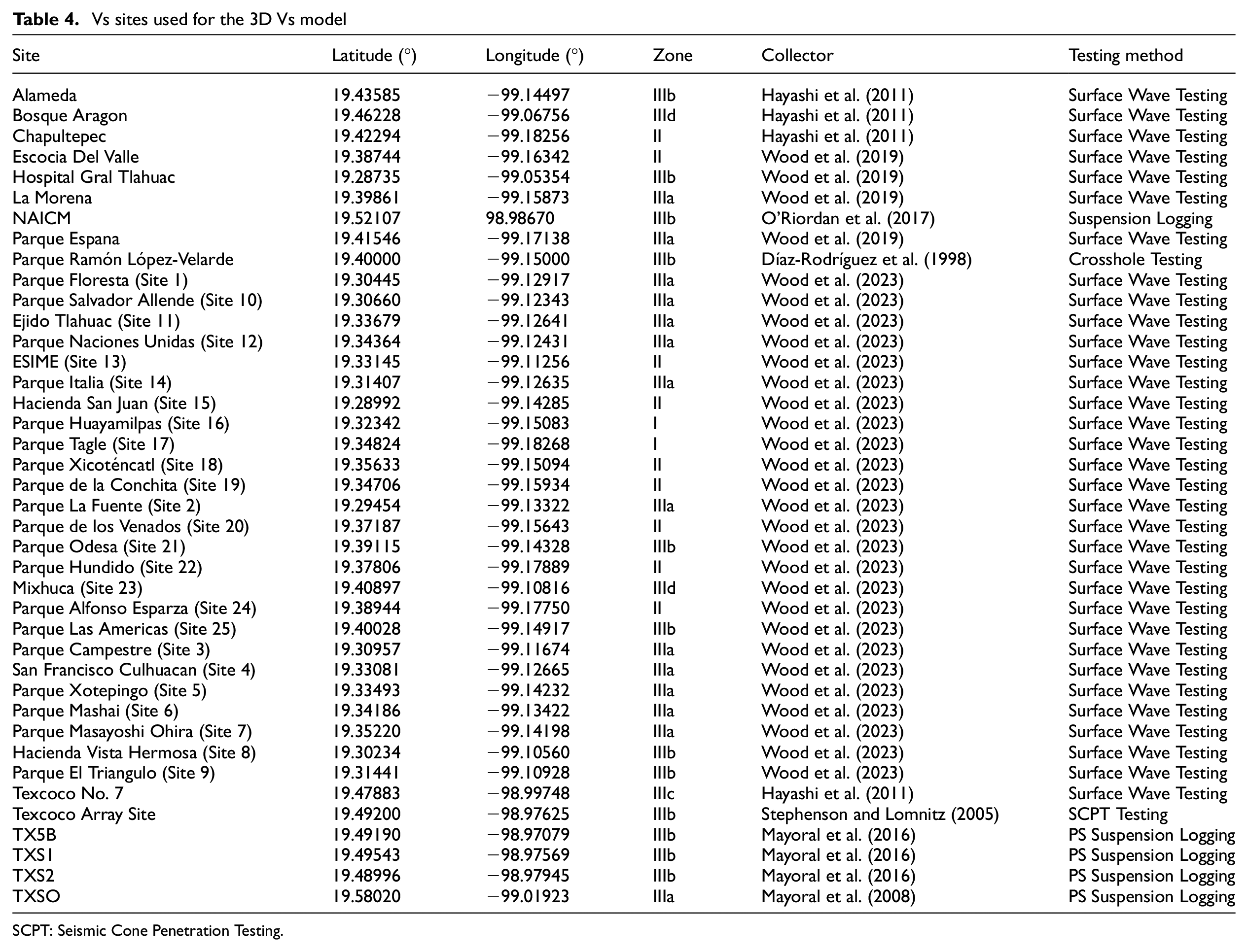
SCPT: Seismic Cone Penetration Testing.

In the first step, all the Vs profiles gathered in this study were broken up into five generalized soil layers plus bedrock according to major breaks in the Vs profile and general layering provided by Díaz-Rodríguez et al. (1998): Desiccated Crust, Upper Clay, Lower Clay, Lower Coarse Grain, Deep Coarse Grain, and bedrock. Each layer was generally separated based on the Vs and depth of the layer in the Vs profile with characteristics used to define each layer described below. It should be noted that the Upper Coarse Grain layer, shown in Santoyo et al. (2005) and Figure 1, was not included in the model as this layer was so thin that it could not be resolved effectively in many of the Vs profiles used in the study. In the next step, the termination depth and the average Vs of each layer were determined. If a layer was determined to contain multiple adjacent soil layers, the time-averaged Vs of the layers was used as the final representative Vs of those layers.

The 3D Vs model is formed by (1) a Desiccated Crust layer, which is defined as the layer of soil that extends from the surface to a termination depth where the next major Vs change occurs (typically an inverse (lower) velocity layer). Some of the sites did not have the Desiccated Crust layer because the testing method used could not resolve or test the first few meters of soil (i.e. PS suspension logging or Seismic Cone Penetration Testing (SCPT)). The Desiccated Crust layer generally has a Vs of ∼100–200 m/s and a termination depth less than 5 m; (2) the Upper Clay layer, which is currently considered as crucial to understand the site effect in the Basin, is located directly below the Desiccated Crust layer in most of the shear wave velocity profiles. The Upper Clay layer is very soft with a Vs ranging between 45 and 100 m/s; (3) the Lower Clay layer, which is defined as the single soil layer, or the combination of soil layers, between the termination of the Upper Clay layer (Vs greater than ∼100 m/s) and the beginning of the Lower Coarse Grain layer (i.e. the impedance boundary). While this layer is named the Lower Clay Layer, in Zone II near the edge of the basin, this layer is an interlayered mixture of clay, silt, and sand. As discussed previously, the Upper Coarse Grain layer is not included in the model as its thickness is typically between 1 and 3 m making it too thin to resolve easily for many investigation methods. The Upper Coarse Grain layer typically has a Vs of 300–400 m/s. The Lower clay layer termination depth was estimated from the measured natural site period (T_N) and the average Vs of the sediments above the Lower Coarse Grain layer (V_S,avg) using the equation H = (T_N * V_S,avg)/4; and (4) the Lower Coarse Grain layer is defined as the soil layer, which directly follows the Impedance boundary generally with a Vs above 300 m/s. This layer terminates at the end of the Vs profile, the beginning of the Deep Coarse Grain layer, or the beginning of the bedrock layer. However, if the Vs profile from a particular site ended with the Lower Coarse Grain layer, the termination depth of the Lower Coarse Grain layer was unable to be obtained (i.e. at the center of the Basin with thick clay layers); (5) the Deep Coarse Grain layer is defined as the single soil layer, or combination of soil layers, between the end of the Lower Coarse Grain layer and the beginning of the bedrock layer. For some of the sites, the Deep Coarse Grain layer’s termination depth was beyond the Vs profile’s termination depth. Like the Lower Coarse Grain layer, if the Deep Coarse Grain layer was the last layer in the Vs profile, the depth of the Deep Coarse Grain layer was unable to be obtained. The bedrock layer is defined as the layer where the shear wave velocity exceeded a value of 700 m/s. It is sometimes called “the engineering bedrock.” The bedrock layer did not contain a final termination depth value since it was the last defined layer for the model. In most cases, the bedrock layer was not present in the Vs profiles for the sites located in Zone IIIb through Zone IIId. Since the bedrock layer was limited in data and the final layer in the system, termination depth and Vs data points were not derived for this layer. It should be mentioned that the five generalized layers discussed above were not observed in all the sites used in this study. In addition, the complex geology of the Basin is being significantly simplified into these five primary layers. The intermixing of soil types and changes in soil composition from Zones II and III, are considered in future modeling with Vs changes due to period. However, the simplicity of the model accounts for Vs changes, but not soil type changes directly. To the best of the authors’ knowledge, this type of shallow layered model (3D Vs) has not been assembled before for Mexico City. This description allows for a quantitative treatment in terms of the site period which demonstrates significant trends in the model parameters. This result can be further validated and improved as more data become available.

Results and discussions

Data variability and trends

Statistical analysis was performed to understand the variability and general trends of the Vs model data. The analysis targeted the variability for both the termination depth and Vs of each layer defined in the Vs profile. Figure 3 depicts the box and whisker plots of the Vs data used for the 3D Vs model for each layer. A box-and-whisker plot may be regarded as a graphical display of data variation in data categories. It is essentially a compact display of histograms of multiple sets of data in the same graph showing the median, the upper and lower quartiles and the standard deviation. It is helpful for easier judgment and allows for effective analysis. These plots are categorized based on the seismic zonation defined in the NTC (2004) to highlight areas where the most significant variability of the input data is observed and to identify any trends in the data. Zone I was excluded from the figure due to incompatibility with other zones and a lack of sites in Zone I. Zone IIIc and Zone IIId were combined because of the limited sites present in these zones.

Figure 3.

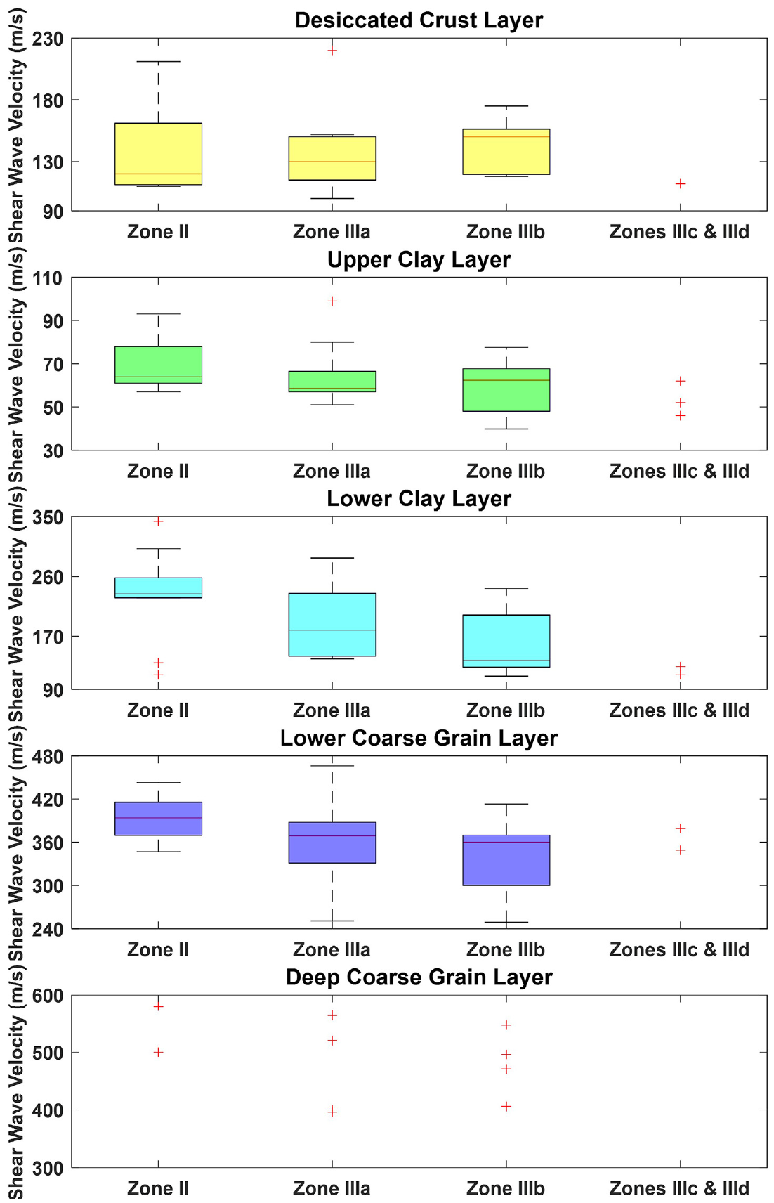
Box and whisker plots for the Vs data used in the 3D Vs model categorized by seismic zonation.

To discuss the data variability and trends in relation to the site period, one should understand the representative site period for each seismic zone. According to the NTC (2004) site period map, Zone II represent site periods between 0.5 and 1.0 s, Zone IIIa represents site periods between 1.0 and 1.5 s, Zone IIIb represents site periods between 1.5 and 2.5 s, Zone IIIc represents site periods between 2.5 and 3.5 s, and Zone IIId represents site periods greater than 3.5 s. Therefore, the site period increases from Zone II to Zone IIId (i.e. from left to right in Figure 3).

From Figure 3, the range and variability of the Desiccated Crust layer Vs data are generally consistent between the zones, with no upward or downward trend in Vs with median values between 100 and 150 m/s. To evaluate the quality of the data for fitting a modeling equation, the interquartile range (IQR) value was normalized by the median for each zone. The normalized IQR values range from 20% for Zone IIIb to 35% for Zone II for the Desiccated Crust layer. A large percentage, such as 35%, indicates that the Desiccated Crust layer Vs data variation is significant. This is expected given the different near-surface conditions throughout the Basin. The Upper Clay layer Vs data in Figure 3 follows a downward trend as the site period increases moving toward the center of the Basin. This is likely caused by the intermixing of clays, silts, and sands toward the edge of the basin (i.e. Zone II). The median Vs of the Upper Clay layer is between 50 and 65 m/s. The normalized IQR values for the Upper Clay layer range from 12% for Zones IIIc and IIId to 26% for Zone IIIb. These values of the normalized IQR for the Upper Clay layer are less than the range in the Desiccated Crust layer. Similar to the Upper Clay layer, the Lower Clay layer Vs data follows a decreasing trend as the site period increases. Also, similar to the Upper Clay Layer, this trend is likely caused by the intermixing of clays, silts, and sands toward the edge of the basin (i.e. Zone II). The median Vs for this layer ranges from 234 m/s at the edge of the Basin to 118 m/s toward the center. Its corresponding normalized IQR values range from 5% for Zones IIIc and IIId to 51% for Zone IIIa. Generally, the normalized IQR values for the Lower Clay layer are greater than those for the Desiccated Crust and Upper Clay layers, suggesting the Lower Clay layer has more variability likely due to differences in consolidation of the layer across the Basin and additional intermixing of soil layers in this zone. The Lower Coarse Grain layer Vs data also follows a decreasing trend as the site period increases moving toward the center of the Basin. The median Vs vary from 394 m/s at the edge of the Basin to 349 m/s at the center of the Basin for this layer. The normalized IQR values of this layer range from 10% for Zone II to 20% for Zones IIIc and IIId. In general, these values of the normalized IQR for the Lower Coarse Grain layer are less than the normalized IQR values for other layers. The Deep Coarse Grain layer Vs data is generally consistent across zones. The median Vs of this layer varies from 480 to 540 m/s. The normalized IQR values range from 7% for Zone II to 29% for Zone IIIa. In general, these values of the normalized IQR for the Deep Coarse Grain layer are similar to the values for the Lower Coarse Grain layer.

Overall, for all layers except for the Desiccated Crust layer, a decreasing trend was observed for the Vs as the site period increases, moving toward the center of the Basin. This is reasonable because as the stiffness of the layers is reduced, the site period increases. It should also be highlighted that the different variability of the data should not disproportionately affect the performance of a modeling equation in any single zone since the general range of the normalized standard deviations and the normalized IQR values for all the zones are relatively close.

Presented in Figure 4 are the box and whisker plots for the depth data used for the 3D Vs model for each layer. These plots are categorized based on the seismic zonation defined in the NTC (2004) map. From this figure, the range and variability of the Desiccated Crust layer depth data are generally consistent between different seismic zones, with no upward or downward trends. The median termination depth of the Desiccated Crust layer is approximately 2 m from the ground surface. The normalized IQR values range from 43% for Zone IIIb to 90% for Zone II. A value of 90% is considerably large; thus, these variations create a less than ideal data set to fit a modeling equation. The Upper Clay layer termination depth data follows an increasing trend as the site period increases. The median termination depths vary significantly (from 10 to 40 m) from the edge of the basin to the center. The normalized IQR values range from 12% for Zones IIIc and IIId to 26% for Zone II. These values of normalized IQR are less than the normalized IQR values present in the Desiccated Crust layer termination depth data.

Figure 4.

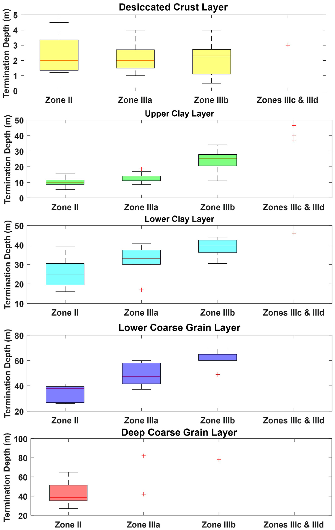
Box and whisker plots for the termination depth data used in the Vs model categorized by seismic zonation.

The Lower Clay layer termination depth data also follows an increasing trend as the site period increases. The median termination depth varies significantly from 25 m at the edge of the Basin to 46 m at the center. The normalized IQR values range from 10% for Zone IIIb to 30% for Zone II. These values of normalized IQR are approximately equivalent to those of the Upper Clay layer. The normalized IQR values are greater in Zone II and decrease to Zone IIIb, alluding to increasing variability of the Lower Clay layer termination depth data in the lower site period zones. This is the result of the layer’s definition, as the termination depth of the Lower Clay layer is the Lower Coarse Grain boundary. In the lower site period zones such as Zone II, the Lower Coarse Grain boundary is more difficult to detect due to the uniformity of the stiffness of the subsurface. This difficulty led to more potential error in the exact location of the Lower Coarse Grain boundary (i.e. the termination depth of the Lower Clay layer). The Lower Coarse Grain layer termination depth data follows an increasing trend as the site period increases. The median termination depth for the Lower Coarse Grain layer varies from 38 m at the edge of the Basin to >60 m at the center. The normalized IQR values of this layer vary from 6% for Zone IIIb to 32% for Zone IIIa.

Similar to most of the other layers, the Deep Coarse Grain layer termination depth data follows an increasing trend as the site period increases. The median termination depth for this layer varies between 39 and 78 m. The normalized IQR values of this layer vary from 23% for Zone II to 32% for Zone IIIa. These values of normalized IQR are greater than the normalized IQR values present in the termination depth data for the other layers, suggesting that the termination depth data for the Deep Coarse Grain layer has a greater level of variability.

Overall, for most of the layers, an increasing trend of termination depth was observed moving toward the center of the Basin. This is expected because as the thickness of the layer becomes greater, the site period increases. From Figures 3 and 4, it was determined that the Vs and termination depth of the Upper Clay layer change significantly within the Basin. Such variations in the Upper Clay layer Vs and termination depth (i.e. thickness) within the Basin need to be accurately taken into account for seismic design of buildings, given that the clay layers are the one of the most important layers influencing the site effects in the Basin. More information regarding the data variability and trends was provided in Rieth (2021).

Site period map evaluation

The site period map evaluation of the Mexico City Basin is presented in Figure 5. Shown in Figure 5a to e are (a) an relief map of the Basin where the site period contour maps are located, (b) percent error for individual points between the NTC (2004) predicted site period map and the measured site periods, (c) site period difference between the NTC (2004) and Lermo et al. (2020) site period map, (d) NTC (2004) and Lermo et al. (2020) site period contour maps, and (e) percent error between Lermo et al. (2020) site period map and measured site periods, respectively. The percent error between each site’s measured site period and the site period maps are presented as colored symbols in the figure. The percent error was calculated using the following equation:

% Error = \frac{(T_{map}) - (T_{M})}{(T_{M})} * 100

where T_map is the map predicted site periods from the NTC (2004) or Lermo et al. (2020), and T_M is the measured site period. Therefore, a positive error indicates that the site period map overestimates the measured site period and vice versa. From Figure 5b, the positive percent errors (warm colors) are mainly concentrated in the Basin’s western edge between the 1.0 s contour and the 3.5 s contour lines. These percent errors match well with the results from Wood et al. (2023), Wood et al. (2019), and Arroyo et al. (2013). According to these studies, the site period is getting shorter in that portion of the Basin due to the consolidation of the very soft lacustrine clay layer over time. The points with a negative percent error (cool colors) are concentrated along the Basin’s western edge between the 0.5 s and 1.0 s contour lines, indicating that the NTC (2004) map underestimates the site periods for this region. These areas represent locations where the site period contour map from the NTC (2004) needs to be revised based on new site period measurements.

Figure 5.

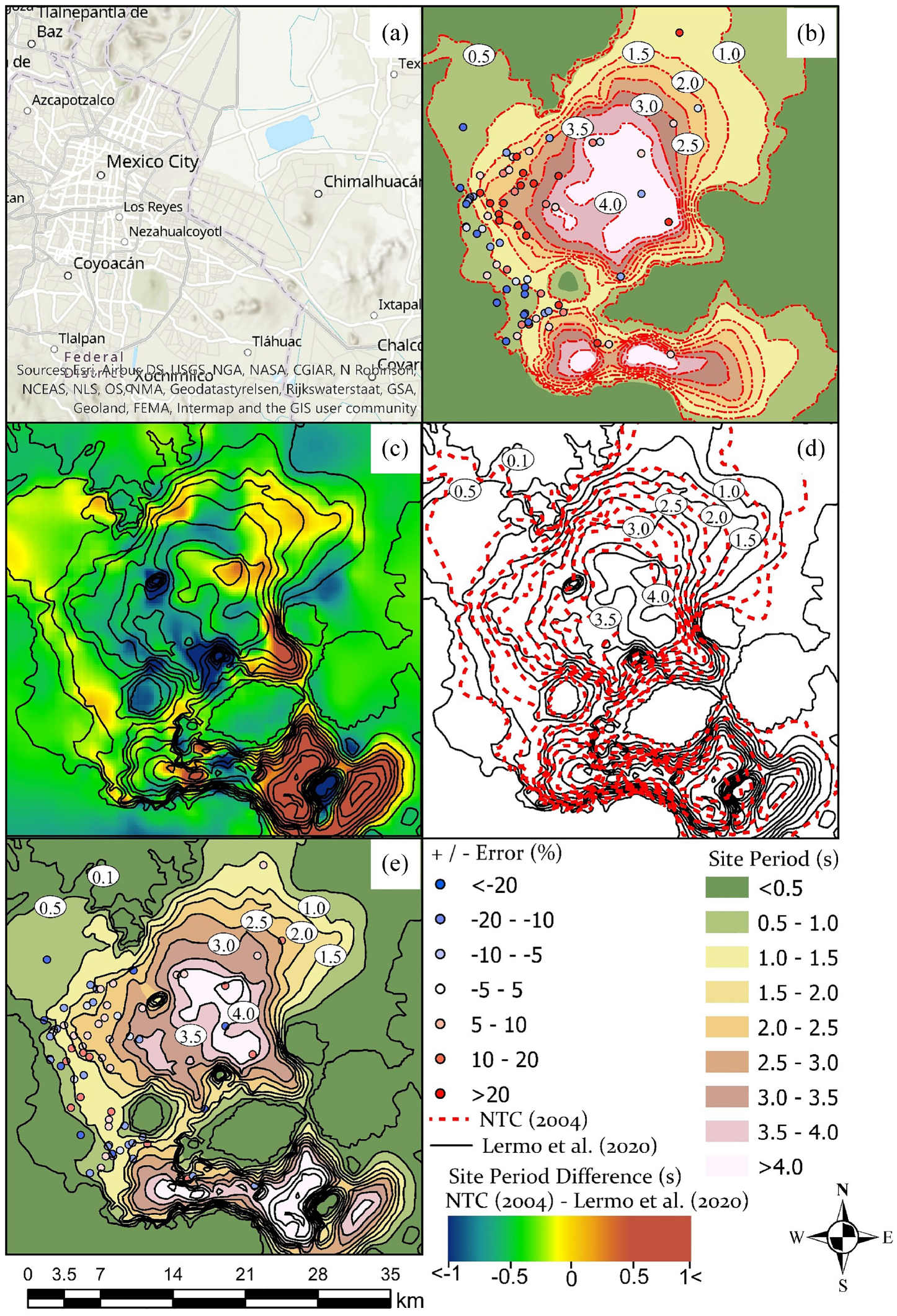
Site period map comparison: (a) relief map of the Basin where the site period contour map is located, (b) percent error for individual points between the NTC (2004) predicted site periods and the measured site periods, (c) site period difference between the NTC (2004) and Lermo et al. (2020) site period prediction maps, (d) NTC (2004) site period contours versus Lermo et al. (2020) contours, and (e) percent error between individual points between measured site periods and Lermo et al. (2020) site period predictions.

In Figure 5c, the differences between the predicted values from the NTC (2004) and the Lermo et al. (2020) site period map are presented to highlight the areas where significant differences are observed. This map was derived by subtracting the Lermo et al. (2020) site period map from the NTC (2004) map. The blue regions represent a difference in site period of more than +1.0 s, while the dark brown regions represent a site period difference of more than −1.0 s. The yellow color represents an area where the NTC (2004) and the Lermo et al. (2020) site period map are equivalent with green and orange colors representing slight differences between the maps. The most significant differences are observed in the southern lakebed where the NTC (2004) map has less detail. Many areas in the map show only minor differences between the maps indicating general good agreement. In Figure 5d, the NTC (2004) site period map (red) is overlain on the site period contours developed by Lermo et al. (2020). Similar to Figure 5c, general good agreement between the maps is observed, with the largest differences observed in the southern lakebed.

The Lermo et al. (2020) site period map is presented in Figure 5e, with the locations of the measured site periods color-coded according to the error between the measured and predicted values. In general, similar underestimates and overestimates are observed between the Lermo et al. (2020) map and the measured sites, as the NTC (2004). However, the errors tend to be lower (closer to 0) for the Lermo et al. (2020) predictions.

To understand the overall performance of the site period prediction maps, box and whisker plots for the error between the measured site periods and the NTC (2004), Lermo et al. (2020), and SASID (2020) site periods are shown in Figure 6. In general, each of the site period prediction methods have no bias in the predictions with the others having an average error near to zero. However, it is clear that the Lermo et al. (2020) and SASID (2020) predictions generally have lower standard deviations than the NTC (2004).

Figure 6.

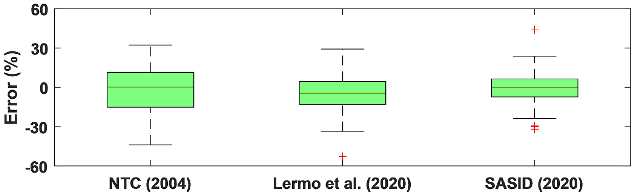
Box and whisker plots for the error between the measured site periods and the NTC (2004), Lermo et al. (2020), and SASID (2020) site periods.

3D shear wave velocity model

Shown in Figure 7 are the final models for the Vs and termination depth of each layer for the Mexico City Basin. In order to fit the Vs and termination depth data sets, multiple functional forms were explored, with the most appropriate function chosen in the final model. The modeling equations were derived from the finalized data sets gathered from the Vs profiles and site periods from all the sites. Splitting the data between the North and South lake beds or other separations throughout the Basin was considered but resulted in a poorer quality model. In the final models, the site period is used as the only input variable. While more complex models (e.g. site period = f (Vs, Depth)) could have been used, in this study, efforts were made to generate a simple 3D model for the Vs in the Basin, so users can generate the Vs profile with a minimal number of inputs. Therefore, given that the site period within the basin can be determined from the available site period prediction maps (or directly measured using MHVSR), the site period was used as the only input for the 3D Vs model. This means that using the site period for a location within the Basin and the models developed in this study, one can construct a Vs profile by estimating the Vs and termination depth of each layer. The final modeling trends and their upper and lower standard deviation curves are also presented in Figure 8 show a reasonable range in which the predicted Vs and termination depth values could exist.

Figure 7.

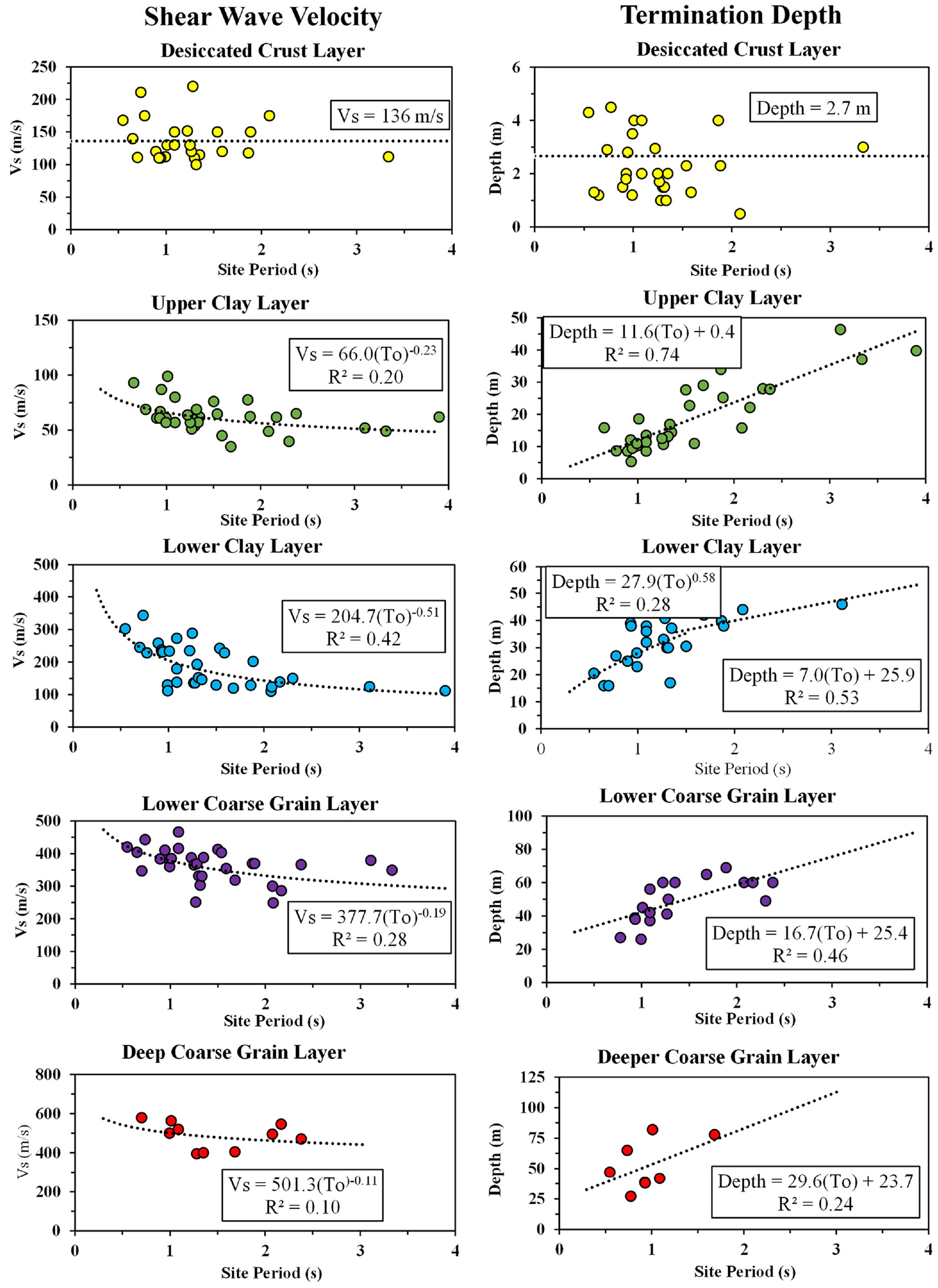
Shear wave velocity and termination depth final models for the Mexico City Basin.

Figure 8.

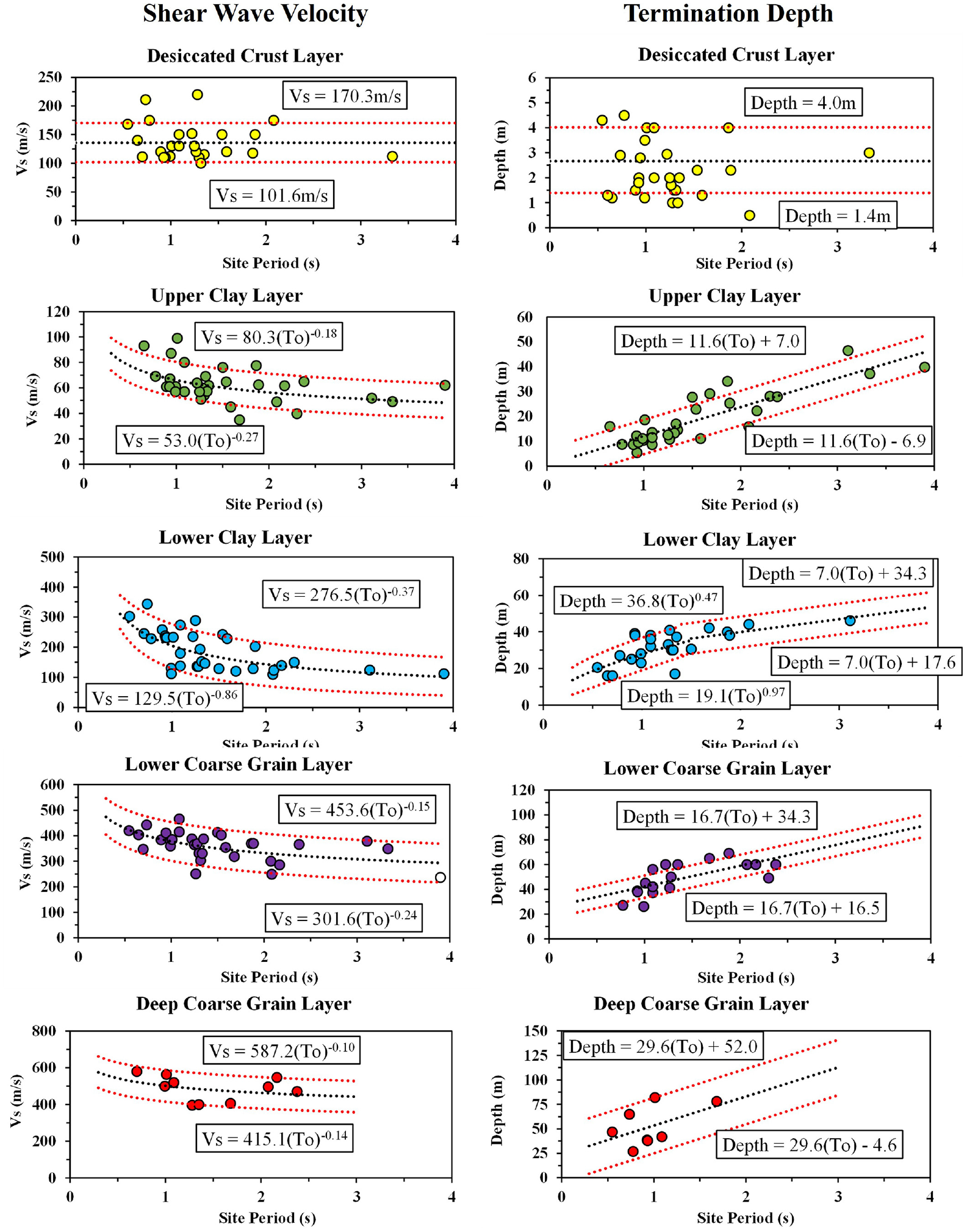
Upper and lower bound model equations (red dotted lines) for the shear wave velocity and termination depth for each layer for the Mexico City Basin.

The Vs and termination depth for the Desiccated Crust layer were determined to be independent of the site period; hence the average of the termination depth and Vs data points was assigned. Assigning one constant value for the termination depth and Vs of the Desiccated Crust layer might result in some inherent issues with accuracy. However, since the Desiccated Crust layer is so thin, these errors were considered marginal; therefore, they should not present a major problem with the validity of the model as a whole.

The Vs modeling equation for the Upper Clay layer is based upon a power function, while the termination depth equation is based on a linear equation. The R² for the Vs of the Upper Clay layer is 0.20 and considered poor. The R² for the termination depth of the Upper Clay layer is 0.74, which is a much better fit. The Upper Clay layer contains many points across the site period spectrum for both termination depth and Vs modeling equations. More specifically, the data ranges from a site period of 0.65–3.90 s for both the Vs and termination depth equations. Unlike the other layers, the Upper Clay layer was present at the majority of the sites.

For the Lower Clay layer, the Vs prediction equation is presented as a power function, but unlike the Upper Clay layer, the termination depth prediction equation is presented as a combination of a linear and power equation. The termination depth equation is a two-part equation where the termination depth of any site with a site period <1.5 s is predicted by the power function, and any site with a site period ≥1.5 s is predicted by the linear equation. This two-part equation was determined to be the best representation of the depth to the Lower Clay Layer boundary as the thickness of the impendence boundary decreases rapidly for longer site periods. The termination depth of the Lower Clay layer in the shorter site period zones is very shallow and rapidly increases as the site period increases, hence the inclusion of the power function for shorter site periods. The rapidly increasing depth leveled off at a site period of 1.5 s, and no longer followed the projection of the power function. The R² for the Vs of the Lower Clay layer is 0.42, which indicates a moderate fit. The two trend lines for the termination depth of the layer have R²s of 0.28 and 0.53, which indicate poor to moderate fits to the data. The data ranges from a site period of 0.55–3.9 s for the Vs equation and 0.55–3.1 s for the termination depth equation. The difference in range is due to the Lower Clay layer being the final layer in the Vs profile for the 3.9 s site; therefore, a final termination depth value could not be obtained.

The Vs prediction equation for the Lower Coarse Grain layer is a power function, while the termination depth prediction equation is linear. The R² for the Vs trend is 0.28, which indicates a poor fit to the data. For the termination depth, the R² for the trend is 0.46, indicating a moderate fit. The distribution of data points for the termination depth modeling equation is relatively small, with data points limited between 0.78 s and 2.38 s. The shear wave velocity data points are better distributed, with data ranging from 0.55 s to 3.33 s. Similar to the Lower Clay layer, the range of the Vs data for the Lower Coarse Grain layer is greater than the range of the termination depth data due to some of the sites terminating within the Lower Coarse Grain layer.

The Vs modeling equation for the Deep Coarse Grain layer is in the form of a power function, and the termination depth modeling equation is in the form of a linear function. The Deep Coarse Grain layer’s equations have limited data points for both the termination depth and Vs equations. This is because, for some of the sites, the Lower Clay or the Lower Coarse Grain layer was the last layer of the Vs profile. The R² for the Vs trend is 0.10, which indicates a very poor fit due to the limited data with large variabilities. The R² for the depth trend is 0.24, which indicates a poor fit. The site periods associated with the data for the Vs and termination depth equations range from 0.70 s to 2.4 s and 0.55 s to 1.7 s, respectively.

Comparisons between measured and predicted vs profiles

The performance of the 3D Vs model is analyzed by generating two representative cross-sections to show the change in Vs geospatially across the Basin. Figure 9 shows the Lermo et al. (2020) site period prediction contour map along with the two cross-sections of A-A’ and B-B’ that illustrate the variation of the Vs along two lines in the Basin. The cross-sections depicted in Figure 9 are developed using the Vs model and site periods derived from the Lermo et al. (2020) site period map. Generally, the cross-sections generated using the 3D Vs model identify many of the essential characteristics of the Basin that were determined by past studies. These characterizations include, but are not limited to: an increase in the thickness of the Upper Clay layer with increasing site period, a slight decrease in the Upper Clay layer’s shear wave velocity as one moves from the edge of the Basin toward the center, an overall decrease in stiffness from all the layers toward the center of the Basin (i.e. decrease in overall Vs), and a constant Desiccated Crust (2.7 m thick) layer throughout the entire basin.

Figure 9.

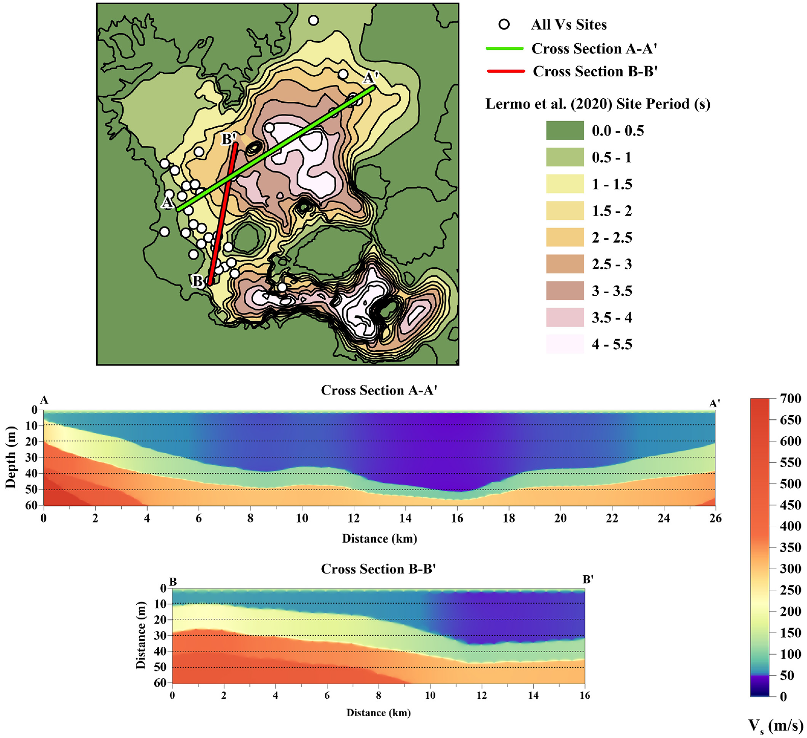
Example of shear wave velocity cross-sections developed using the 3D Vs model and site periods derived from Lermo et al. (2020).

In order to present a clearer comparison between the measured and predicted Vs profiles, several sites along the cross-sections A-A’ and B-B’ are presented in Figures 10 and 11, respectively. Sites shown in Figure 10 include Parque Floresta, Parque La Fuente, Parque Italia, San Francisco Culhuacán, Ejido Tláhuac, and Mixhuca, while sites presented in Figure 11 include Parque Odesa, Parque Alfonso Esparza, Parque Las Américas, Ramón López Velarde Park, TXS1, and TXS2.

Figure 10.

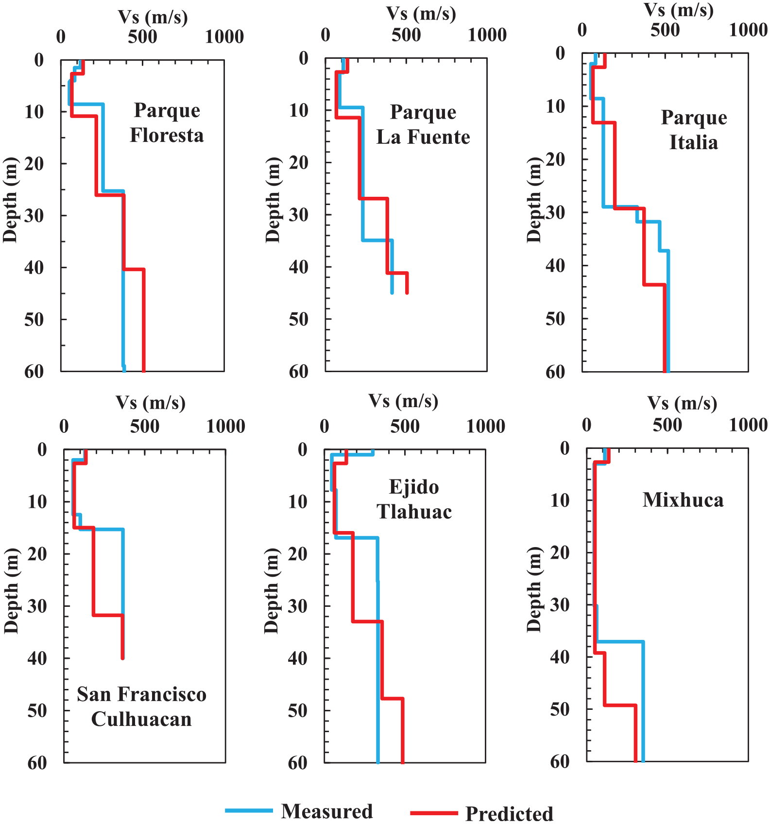
Predicted (red) and measured (blue) Vs profiles for sites located along cross-section A-A’.

Figure 11.

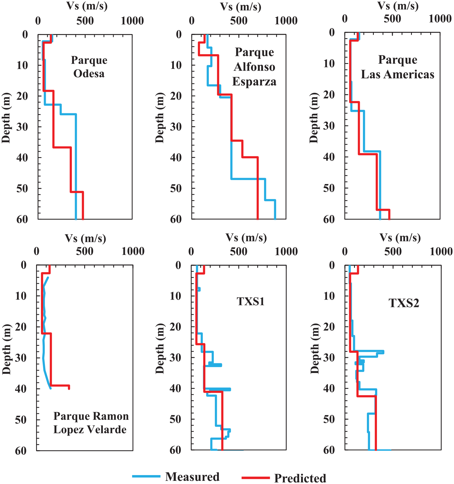
Predicted (red) and measured (blue) Vs profiles for sites located along cross-section B-B’.

From Figures 10 and 11, it is clear that the model accurately predicts the measured Vs profiles in most areas by precisely capturing most of the layers and their associated Vs, but it has some discrepancies. It is important to determine why these discrepancies occur and provide possible remediation strategies to resolve them.

Due to the model’s mathematical structure, all the layers are required to exist in all zones, even if the measured Vs profile does not contain all of them. For example, in Figure 10, San Francisco Culhuacán, Ejido Tlahuac, and Mixhuca do not contain a Lower Clay layer, but the predicted Vs profile unavoidably includes this layer. Nevertheless, as the depth increases, the model provides a reasonable comparison with the measured Vs. Another case of predicting a layer that does not exist is in Figure 11 for Parque Alfonso Esparza, located in Zone II. Due to the location of Zone II being around the edges of the Basin, the presence of the Upper Clay layer can diminish or completely vanish. This diminishing Upper Clay layer is observed in Figure 9 between 0 and 2 km in cross-section A-A’. Nevertheless, the predicted Vs profile for Parque Alfonso Esparza contains a very thin Upper Clay layer because the model is unable to neglect this layer. In order to remove these types of discrepancies, layers were removed at certain site period thresholds (i.e. the bedrock layer and Deep Coarse Grain layer), but this was only performed if a majority of the sites under the threshold did not contain the layer. For Parque Alfonso Esparza, the prediction of the Upper Clay layer is inevitable, and the generality of the model is unable to cope with the uniqueness of the site. This type of discrepancy is bound to happen all over the Basin and is unavoidable with the current structure of the 3D Vs model. To resolve these discrepancies, a completely different and more complex function for the Vs model would be necessary, which would require more inputs and data to properly develop which are not currently available.

Layer interface discrepancies occur when the model incorrectly predicts the termination depth of one layer, causing some overlap between the predicted and measured layers. These discrepancies are observed in Figures 10 and 11. For instance, in Figure 10, Parque La Fuente predicts the bottom of the Lower Clay layer at a depth of 27 m, but the measured profile does not show the bottom of the layer until 35 m. The model accurately predicts the Vs of the Lower Clay layer and the Lower Coarse Grain layer, therefore classifying this inaccuracy as a layer interface discrepancy. More examples of layer interface discrepancies are presented in Figures 10 and 11 for Parque Floresta, Parque Italia, and Parque Las Américas, at depths of 9, 37, and 25 m, respectively. Similar to the prediction of layers that do not exist, the model’s simplicity prohibits the flexibility for sites that present uniqueness from other sites with similar site periods. These inaccurate predictions are the result of the termination depth prediction equations and could be mitigated by the use of more data or the use of a more complex modeling method.

Another issue associated with the ability of the model to accurately predict the Vs profile of a given site is the overestimation or underestimation of the Vs of any given layer. For example, in Figure 10, the predicted Vs profile for Parque Italia estimates the Vs for the Lower Clay layer (depth = 13 m) to be 196 m/s, but the measured Vs of the Lower Clay layer is roughly 128 m/s. Other examples of this type of inaccuracy are presented in Figures 10 and 11 for Mixhuca, TXS2, and Parque Alfonso Esparza, at depths of 50, 28, and 47 m, respectively. These errors are likely the result of the large variations in the source data used to derive the modeling equations. The model is unable to cope with large variability and uniqueness between sites with similar site periods. More sites need to be included in the model to further improve its ability to provide accurate results everywhere in the Basin and mitigate this issue.

In general terms, according to the comparison made between the predicted and measured Vs profiles in Figures 10 and 11, it is apparent that the 3D model developed in this study is capable of capturing most of the layers and their associated Vs for the Mexico City Basin. Particularly, the model performs quite well in predicting the Vs and thickness of the Upper Clay layer, which is the most critical soil layer in the Basin, as illustrated in Figures 10 and 11. It is worth mentioning that due to the generalization of the layers, there are inherent errors embedded into the model, as discussed above. More comparisons of the measured versus predicted Vs profiles were provided in Rieth (2021).

Modeling errors

To better examine the performance of the 3D Vs model for predicting the Vs profile at any given location within the basin, normalized residuals between the predicted and measured Vs profiles are calculated. The results of the normalized residual plots are shown in Figure 12, with the original Vs profiles and time-averaged Vs profiles presented in the left and right columns, respectively. These normalized residual plots are organized by seismic Zone to delineate areas where the model excels or needs improvement. Zone IIIc and Zone IIId were excluded from the normalized residual plots because they contain a total of three sites.

Figure 12.

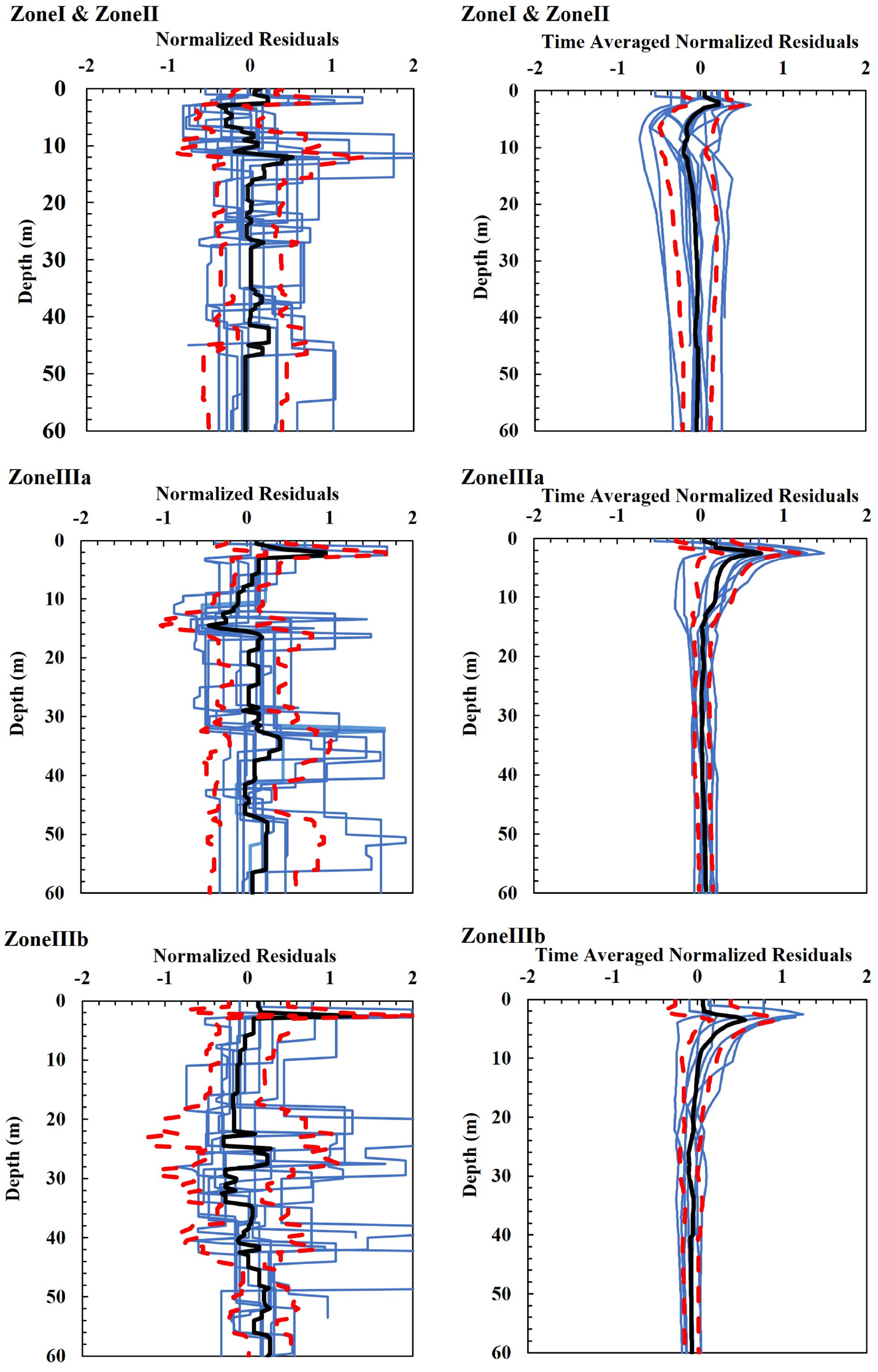
Normalized residuals plots between the predicted and measured Vs profiles categorized by seismic zone. The original and time-averaged normalized residual plots are presented in the left and right columns, respectively. Blue lines represent individual residual profiles, black lines represent the median, and the red lines represent plus and minus one standard deviation from the median.

To develop the normalized residual plots for the original Vs profiles, the Vs model was used to predict the Vs profiles for each site. The modeled Vs profiles were then subtracted from the measured shear wave velocity profiles to obtain the residual versus depth profile. The residual profiles were then normalized with respect to the measured Vs profile. Similar steps were followed to create the time-averaged residual profiles. The individual normalized residual and time-averaged normalized residual profiles for each site are depicted with blue lines in Figure 12. To better understand the variability of the normalized residuals for all the sites in each Zone, the standard deviation (σ) and the median were also calculated. The median (the solid black line) and plus and minus one standard deviation (two red dashed lines) profiles for the normalized residual and time-averaged normalized residual profiles are presented in the left and right columns of Figure 12, respectively.

Large spikes in the median normalized residual profile are present mainly in the original profiles in Figure 12. For example, the normalized residual plots in Figure 12 contain a large spike in the median normalized residual profile at a depth of ∼3 m. These shallow spikes are the result of inaccuracies of the model for predicting the Desiccated Crust-Upper Clay layer interface. Despite these large spikes not being present at other depths in the time-averaged normalized residual median profiles, the large spikes occur at various other depths in the normalized residual median profiles. In Zone II, a series of large spikes in the median normalized residual profile are present at 2.5, 13, and 37 m. In Zone IIIa, a series of large spikes in the median normalized residual profile is present at 1, 15, 35, and 50 m. In Zone IIIb, a series of large spikes in the median normalized residual profile are present at 3, 26, and 33 m. It is important to mention that the normalized residual spikes are not sustained with depth, suggesting that these errors are localized to layer interface discrepancies.

Based on the definitions of the layers and the modeling equations for each layer, the difference in Vs between any two adjacent layers is large. Furthermore, if the depth equation for a given layer overestimates the measured depth of the same layer, large normalized residuals that may be disproportionally higher are expected. For example, the Upper Clay layer Vs is disproportionately low compared to the Desiccated Crust and Lower Clay layers (up to 2× less in Vs); therefore, large jumps in residuals are expected in the Desiccated Crust-Upper Clay layer interface. More specifically, if for one depth the predicted Vs is 135 m/s (predicted Desiccated Crust layer velocity), yet the measured shear wave velocity is 50 m/s (Upper Clay layer velocity), a residual of −85 m/s is to be expected. Despite it being normalized to the measured value of 50 m/s, this would still leave a value of 1.7. This creates large jumps in normalized residuals, which is disproportional to any other area in the Vs profile. The large spike at 3 m in the time average normalized residual plots is attributed to this disproportional behavior between the shear wave velocities of the two layers. Furthermore, the smoothing nature of the time-averaged Vs profiles creates less Vs difference between layers, therefore removing the large spikes associated with layer interface discrepancies. The smoothing behavior of the time-averaged Vs profiles is less effective at removing the Desiccated Crust-Upper Clay layer discrepancy due to the shallow depth and drastic difference between the Vs of the two layers. Accordingly, any depth past the 3 m spike in the time-averaged normalized residuals plots shows little to no deviation from zero, unlike the normalized residual plots. Therefore, the large spikes are more applicable to the Desiccated Crust-Upper Clay and Upper Clay-Lower Clay layer interfaces since the interfaces between the other layers have less extreme Vs differences.

From Figure 12, the model is relatively accurate for all depths for Zone II, with the absolute values of the median normalized residual profile being less than 0.1 throughout most of the depths. In addition to the previously discussed spikes of normalized residuals, sustained normalized residuals are present between the depths of 2.5 to 6.5 m and 41 m-47 m. The sustained median normalized residual for the depths between 2.5 m-6.5 m results from inaccuracies in the Upper Clay layer Vs modeling prediction. High normalized residuals for the Upper Clay layer discrepancies for Zones II can be attributed to the smaller thickness of the layer, allowing for larger influences of layer interface discrepancies. In addition, the sustained median normalized residual for the depths between 41 and 47 m results from inaccuracies in predicting Vs of the Deep Coarse Grain layer. The median time-averaged normalized residual profiles are equal to zero for most of the depths for all the zones. Compared to the other zones, the individual site time-averaged residual profiles for Zone II have the most variation, alluding to more uncertainty associated with predicting the Vs profiles in this particular Zone.

From Figure 12, the normalized residual plot for Zone IIIa contains larger residuals than Zone II results. The residuals for Zone IIIa are present in the four large spikes at 1, 15, 35, and 50 m for the normalized residual plots and at 3 m for the time average residual plots. As mentioned, these large spikes are the result of discrepancies in layer interfaces. Despite these interface-induced errors, the plots are mostly centralized around 0, with limited cases of sustained error. This indicates that the model generally performs well in predicting the Vs of each layer for Zone IIIa. Examples of sustained normalized error are observed at depths between 3–13 m, 30–41 m, and 48–56 m. Like Zone II, these errors are associated with discrepancies in the predicted Vs for a specific layer at a given depth. The time-averaged residual median profile for Zone IIIa is almost zero, except for the large spike at 3 m. Compared to Zone II, the time-averaged residual profiles show less data variation and a better concentration of values near or equal to zero.

In Figure 12, Zone IIIb has a more variable distribution of normalized residuals with depth than the normalized residual profiles for the other zones. This variation is highlighted by the drastic change and range of the plus and minus standard deviation. Like the other zones, Zone IIIb contains a large spike in both the normalized residual profiles and time-averaged residual profiles at ∼2 to ∼4 m. The largest sustained spike in the median normalized residual profile takes place between 17 and 30 m, which indicates an issue with the prediction accuracy of the Upper Clay-Lower Clay layer interface. In addition to the spikes in residual, large, sustained residuals occur from ∼46 to 60 m in the normalized residual plots. This sustained error results from the model’s inability to accurately predict the Vs of the Deep Coarse Grain layer. For Zone IIIb, the median time-averaged normalized residual profile is mostly equal to zero after the first spike at 5 m, but the range of the individual profiles is larger than that of Zone IIIa.

Conclusion

This study provides an evaluation of current site period prediction maps and a shallow 3D Vs model for the Mexico City Basin. These were performed and developed using MHVSR and EHVSR measurements and Vs profiles collected in the previous studies.

The NTC (2004) site period prediction map for Mexico City has been shown to both under and over predict site periods compared to the measured values used in this study. However, there seems to be no bias in the predicted values. The Lermo et al. (2020) and SASID (2020) predicted site periods tend to produce lower errors as compared to the NTC (2004) predictions and have little to no bias. However, there are still areas in need of improvement across the Basin where additional measurements would better refine the predicted site periods. Field data is being collected as part of the current studies requested by the Mexico City authorities.

In addition, a shallow 3D Vs model was created to provide future studies with a means to predicting a Vs profile for any site located in the Basin. A total of 40 sites were used to develop the Vs prediction model. The Vs model is divided into a termination depth and Vs modeling equations for five generalized layers. These layers include the Desiccated Crust, Upper Clay, Lower Clay, Lower Coarse Grain, and Deep Coarse Grain layers. The Upper Coarse Grain layer located between the Upper and Lower Clay layers was excluded from the model as it was not resolved in many of the Vs profiles used in the study due to its minimum thickness of 1 to 3 m.

The site period was used as the only input for all the modeling equations in order to simplify the model and maximize its applicability. This feature increases the future applicability of the model to the Basin because as the site periods in the Basin change (due to the consolidation of the lacustrine clay deposit), the model can be modified by utilizing updated site periods, such as the future update to the Lermo et al. (2020) map by Ramos-Pérez et al. (2024), to predict Vs in the Basin. This approach will not be as accurate as remeasuring Vs profiles, but will provide a more accurate result compared to not accounting for the site period changes. It was shown that the model performs well in predicting Vs profiles in most areas. However, due to the generalization of the layers, there are still inherent errors embedded into the model developed in this study. The main errors include layer interface discrepancies, inaccurate prediction of layer Vs, and layers that do not exist. The Vs model is most accurate at predicting the Upper Clay layer depth and Vs compared to other layers. This is important because, according to previous studies (Chávez-García and Bard, 1994; Sánchez-Sesma et al., 1993a), the clay layer is the most influential layer dominating site effects. Moreover, the model performs better in Zone II and Zone IIIa compared to the other seismic zones. Overall, the shallow 3D Vs model developed in this study provides an accurate and valuable tool for understanding the Vs of the Basin and significant input for the 3D physics-based ground motion modeling of the Basin, now in developing stages, like the recent calculation by Hernández-Aguirre et al. (2023) using the spectral element method. It should be mentioned that errors associated with the model are more likely in areas where limited data is available, particularly the areas on the eastern edge of the Basin.

Footnotes

Acknowledgements

H.C.J. thanks CONACYT for currently supporting his postdoctoral fellowship.

Correction (January 2024):

Article updated to correct in-text citation and displayed reference NTC (2004).

Declaration of conflicting interests

The author(s) declared no potential conflicts of interest with respect to the research, authorship, and/or publication of this article.

Funding

The author(s) disclosed receipt of the following financial support for the research, authorship, and/or publication of this article: This work is based on work supported the National Science Foundation through the Geotechnical Engineering Program under grant nos CMMI-1266418, CMMI-1822482, and CMMI-2100889. Any opinion, findings, and conclusions or recommendations expressed in this article are those of the authors and do not necessarily reflect the view of the NSF. Partial support from DGAPA-UNAM Project IN 107720 is appreciated.

Data availability

Shear wave velocity profiles, site periods, and site period maps used for this study are freely available through the www.designsafe-ci.org/ website in the following location: .

References

Aki

(1988) Local site effects on strong ground motion. In: Proceedings of the special conference on earthquake engineering and soil dynamics 2, Park City, UT, pp. 103–155. New York: American Society of Civil Engineers.

Anbazhagan

Sitharam

(2020) Site characterization and site response studies using shear wave velocity. Journal of Seismology and Earthquake Engineering 10(2): 53–67.

Arce

Layer

Macías

Morales-Casique

García-Palomo

Jiménez-Domínguez

Benowitz

Vásquez-Serrano

(2019) Geology and stratigraphy of the Mexico Basin (Mexico City), central Trans-Mexican Volcanic Belt. Journal of Maps 15(2): 320–332.

Arroyo

Ordaz

Ovando-Shelley

Guasch

Lermo

Perez

Alcantara

Ramírez-Centeno

(2013) Evaluation of the change in dominant periods in the lakebed zone of Mexico City produced by ground subsidence through the use of site amplification factors. Soil Dynamics and Earthquake Engineering 44: 54–66.

Baena-Rivera

Sánchez-Sesma

Arciniega-Ceballos

Pérez-Rocha

Cruz-Jiménez

(2023) Ground motion similarities in the valley of Mexico from subduction earthquakes. Bulletin of the Seismological Society of America 113: 1–16.

Baena-Rivera

(2017) Campos difusos generalizados para tomografía de valles aluviales: el caso del Valle de la Ciudad de México. PhD Thesis, Repositorio Institucional de la UNAM. Available at: https://ru.dgb.unam.mx/handle/DGB_UNAM/TES01000760359 (accessed November 2022).

Bard

Bouchon

(1980a) The seismic response of sediment-filled valleys. Part 1. The case of incident SH waves. Bulletin of the Seismological Society of America 70: 1263–1286.

Bard

Bouchon

(1980b) The seismic response of sediment-filled valleys. Part 2. The case of incident P and SV waves. Bulletin of the Seismological Society of America 70: 1921–1941.

Campillo

Gariel

Aki

Sánchez-Sesma

(1989) Destructive strong ground motion in Mexico City: Source, path and site effects during the great 1985 Michoacán earthquake. Bulletin of the Seismological Society of America 79: 1718–1735.

10.

Chávez-García

(27–30 June, 2010) Site response at Mexico City. In: 7th international conference on urban earthquake engineering (7CUEE) & 5th international conference on earthquake engineering (5ICEE), 3–5 March, pp. 81–88. Tokyo, Japón: Tokyo Institute of Technology.

11.

Chávez-García

Bard

(1994) Site effects in Mexico City eight years after the September 1985 Michoacán earthquakes. Soil Dynamics and Earthquake Engineering 13: 229–247.

12.

Chávez-García

Salazar

(2002) Strong motion in central Mexico: A model based on data analysis and simple modeling. Bulletin of the Seismological Society of America 92(6): 3087–3101.

13.

Cruz-Atienza

Tago

Sanabria-Gómez

Chaljub

Etienne

Virieux

Quintanar

(2016) Long duration of ground motion in the paradigmatic valley of Mexico. Nature—Scientific Reports 6: 38807.

14.

Díaz-Rodríguez

Cruz

RLS

Dávila-Alcocer

Vallejo

Girón

(1998) Physical, chemical, and mineralogical properties of Mexico City sediments: A geotechnical perspective. Canadian Geotechnical Journal 35(4): 600–610.

15.

Franke

Candia

Mayoral

Wood

Montgomery

Hutchinson

Morales-Velez

(2019) Observed building damage patterns and foundation performance in Mexico City following the 2017 M7. 1 Puebla-Mexico City earthquake. Soil Dynamics and Earthquake Engineering 125: 105708.

16.

Geotechnical Extreme Events Reconnaissance (GEER) (2020) Geotechnical engineering reconnaissance of the 19 September 2017 Mw 7.1 Puebla-Mexico City Earthquake (Version 2.0 2020). Report No. GEER 055-B. DOI: 10.18118/G6JD46.

17.

NTC (2004) Normas Técnicas Complementarias sobre Criterios y Acciones para el Diseño Estructural de las Edificaciones. Available at: https://paot.org.mx/centro/normas_a/2022/8.pdf (accessed 15 December 2023).

18.

Hayashi

Nozu

Tanaka

Suzuki

Ovando-Shelley

(2011) Joint inversion of three-component microtremor measurements and microtremor array measurements at Mexico City. SEG Technical Program Expanded Abstracts 30: 917–921.

19.

Hernández-Aguirre

Paolucci

Sánchez-Sesma

Mazzieri

(2023) Three-dimensional numerical modeling of ground motion in the valley of Mexico: A case study from the Mw3.2 earthquake of July 17, 2019. Earthquake Spectra 39: 2323–2351.

20.

Kawase

Aki

(1989) A study on the response of a soft soil basin for incident S, P, and Rayleigh waves with special reference to the long duration observed in Mexico City. Bulletin of the Seismological Society of America 79: 1361–1382.

21.

Lermo

Sanchez-Sesma

Pérez

Monroy

Mendez

Cuenca

Gonzalez Rodriguez

Cruz

Gonzalez

Maldonado

Espinoza

Gonzalez

Cruz

Gonzalez

Aragon

Mendez

(2020) Updating of the Seismic Zoning of Mexico City and Surrounding Areas Northern Part. Mexico City, Mexico: Institute for Construction Safety, Government of Mexico City.

22.

Mayoral

Asimaki

Tepalcapa

Wood

Roman-de la Sancha

Hutchinson

Montalva

(2019) Site effects in Mexico City Basin: Past and present. Soil Dynamics and Earthquake Engineering 121: 369–382.

23.

Mayoral

Castañón

Alcantara

Tepalcapa

(2016) Seismic response characterization of high plasticity clays. Soil Dynamics and Earthquake Engineering 84: 174–189.

24.

Mayoral

Romo

Osorio

(2008) Seismic parameters characterization at Texcoco lake, Mexico. Soil Dynamics and Earthquake Engineering 28(7): 507–521.

25.

Molina-Villegas

Jaramillo-Fernández

Piña-Flores

Sánchez-Sesma

(2018) Local generation of love surface waves at the edge of a 2D alluvial valley. Bulletin of the Seismological Society of America 108(4): 2090–2103.

26.

Mooser

(September 1990) Mapeo de estructuras geológicas someras de la Cuenca de México. In: Memorias del Simposio El subsuelo de la Cuenca del Valle de México y su relación con la ingeniería de cimentaciones, a cinco años del sismo. México City, Mexico: Sociedad Mexicana de Mecánica de Suelos.

27.

Nishizawa

Satoh

Lei

Kuwahara

(1997) Laboratory studies of seismic wave propagation in inhomogeneous media using a laser Doppler vibrometer. Bulletin of the Seismological Society of America 87(4): 809–823.

28.

Ordaz

Singh

(1992) Source spectra and spectral attenuation of seismic waves from Mexican earthquakes, and evidence of amplification in the hill zone of Mexico City. Bulletin of the Seismological Society of America 82: 24–43.

29.

O’Riordan

Cañavate-Grimal

Francisco Ciruela

Kumar

(17–22 September, 2017) The stiffness and strength of saltwater Lake Texcoco clays, Mexico City. In: Proceedings of the 19th international conference on soil mechanics and geotechnical engineering, Seoul, South Korea: ISSMGE, pp. 1067–1070.

30.

Pérez-Rocha

Sánchez-Sesma

Flores-Cruz

(1995) Análisis de los datos de la Red Acelerométrica del Valle de México con técnicas espectrales. Revista de Ingeniería Sísmica 49: 21–38.

31.

Pestana

Sancio

Bray

Romo

Mendoza

Moss

RES

Mayoral

Seed

(2002) Geotechnical engineering aspects of the June 1999 central Mexico earthquakes. Earthquake Spectra 18(3): 481–499.

32.

Rahimi

Wood

Wotherspoon

(2020a) Influence of soil aging on SPT-Vs correlation and seismic site classification. Engineering Geology 272: 105653.

33.

Rahimi

Wood

Wotherspoon

Green

(2020b) Efficacy of aging correction for liquefaction assessment of case histories recorded during the 2010 Darfield and 2011 Christchurch earthquakes in New Zealand. Journal of Geotechnical and Geoenvironmental Engineering 146(8): 04020059.

34.

Ramos-Pérez

Lermo-Samaniego

Sánchez-Sesma

Perton Mathieu Álvarez-Monroy

Machado-González

Luna-Cruz

(3–5 March, 2024) Analysis of the variation of microtremor horizontal to vertical spectral ratio (MHVSR) in Mexico City.

35.

Rieth

(2021) Shallow 3D shear wave velocity model and revised site period prediction map for the Mexico City Basin. Master Thesis, University of Arkansas, Fayetteville, AR.

36.

Sánchez-Sesma

Chávez-Pérez

Suárez

Bravo

Pérez-Rocha

(1988) On the seismic response of the valley of Mexico. Earthquake Spectra 4: 569–589.

37.

Sánchez-Sesma

Pérez-Rocha

Reinoso

(1993a) Ground motion in Mexico City during the April 25, 1989 Guerrero Earthquake. Tectonophysics 218: 127–140.

38.

Sánchez-Sesma

Ramos-Martinez

Campillo

(1993b) An indirect boundary element method applied to simulate the seismic response of alluvial valleys for incident P, S and Rayleigh Waves. Earthquake Engineering & Structural Dynamics 22: 279–295.

39.

Santoyo

Ovando

Mooser

León

(2005) Síntesis geotécnica de la cuenca del Valle de México. Mexico City, México: TGC Geotecnia.

40.

Seed

Romo

Sun

Jaime

Lysmer

(1988) The Mexico earthquake of September 19, 1985—Relationships between soil conditions and earthquake ground motions. Earthquake Spectra 4(4): 687–729.

41.

Singh

Lermo

Dominguez

Ordaz

Espinosa

Mena

Quaas

(1988) The Mexico earthquake of September 19, 1985: A study of amplification of seismic waves in the valley of Mexico with respect to a hill zone site. Earthquake Spectra 4: 653–673.

42.

Sistema de Acciones Sísmicas de Diseño (SASID) (2020) Available at: https://sasid.unam.mx/webNormasCDMX/ (accessed 15 December 2023).

43.

Stephenson

Lomnitz

(2005) Shear-wave velocity profile at the Texcoco strong-motion array site, Valley of Mexico. Geofisica Internacional 44: 3–10.

44.

Wang

Shi

Jiang

Yao

Miao

(2018) Estimating site fundamental period from shear-wave velocity profile. Bulletin of the Seismological Society of America 108(6): 3431–3445.

45.

Wood

Deschenes

Ledezma

Meneses

Montalva

Morales-Velez

(2019) Dynamic site characterization of areas affected by the 2017 Puebla-Mexico city earthquake. Soil Dynamics and Earthquake Engineering 125: 105704.

46.

Wood

Woodfield

Rahimi

Rosado-Fuentes

Sánchez-Sesma

Cruz-Jiménez

Mayoral

De La

Rosa D

(2023) Shear wave velocity and site period measurements for the Mexico City Basin following the 2017 Puebla-Mexico City Earthquake. Earthquake Spectra 39: 505–527.

Shallow three-dimensional shear wave velocity model for the Mexico City Basin

Abstract

Keywords

Introduction

Data selection

Data used for site period map evaluation

Data used for the 3D shear wave velocity model

Results and discussions

Data variability and trends

Site period map evaluation

3D shear wave velocity model

Comparisons between measured and predicted vs profiles

Modeling errors

Conclusion

Footnotes

Acknowledgements

Correction (January 2024):

Declaration of conflicting interests

Funding

Data availability

References