Probabilistic approach for seismic microzonation integrating 3D geological and geotechnical uncertainty

Abstract

A novel probabilistic methodology for regional seismic site characterization is proposed and applied to a region with highly heterogeneous surficial geology and varying soil sediment thickness and stiffness. The method combines various sources of geological and geotechnical uncertainties to develop a three-dimensional (3D) shear-wave velocity (V_s) model and evaluate the associated uncertainties. A 3D geological model of the unconsolidated deposits was developed using geostatistical interpolation and simulation methods. Sequential indicator simulations produced a quantitative geologic model that explicitly quantified geological uncertainties based on the likelihood of specific soil types occurring. In situ measurements and multivariate statistical analysis allowed the development of empirical correlations between V_s, geotechnical parameters, depth, and soil types. The resulting 3D V_s values were estimated on the basis of V_s-depth correlations and the probability of occurrence of each soil type. In this approach, the propagated uncertainty was also quantified by considering the combined variance. Seismic microzonation mapping was then conducted by transforming the 3D V_s model into two-dimensional (2D) maps that represent the spatial distributions of the time-averaged shear-wave velocity of the top 30 m (V_s,₃₀) and the fundamental site period (T₀), along with their respective uncertainties using Monte Carlo simulations. The results indicate that microzonation maps and their uncertainties are influenced by the thickness, occurrence probability, and geotechnical properties of soils. The proposed method can be used to assess the probabilistic seismic risk at local and regional scales in areas with geologically and geotechnically complex soil properties.

Introduction

Local site conditions tend to modify the amplitude and frequency of incoming seismic waves (Seed et al., 1976). This phenomenon is known as the site effect, and it depends on the geotechnical (e.g. soil type, shear modulus, and damping ratio) and geological (e.g. stratigraphy, basin topography, and thickness) properties of soil sediments. Site-effect parameters such as the time-averaged shear-wave velocity of the top 30 m (V_s,₃₀) and the fundamental site period (T₀) are reliable proxies for regionally evaluating seismic shaking amplification (Heath et al., 2020; Thompson et al., 2014) and seismic microzonation mapping (Licata et al., 2019; Molnar et al., 2020; SM Working Group, 2015).

Although shear-wave velocity (V_s) is recognized as a simple, effective, and representative parameter for determining site effects, obtaining sufficient direct V_s measurements in regional site characterization studies is challenging. As a proxy, the available geotechnical data represent a useful data source for estimating V_s (Oliveira et al., 2020). In this case, empirical V_s correlations with geotechnical parameters (Mayne and Rix, 1995; Robertson, 2009) or depth (Motazedian et al., 2011; Podestá et al., 2019) are suggested for addressing the scarcity of V_s measurements. However, specific depositional environments, such as the presence of soft sensitive clays, which is frequently observed in Eastern Canada (Locat and St- Gelais, 2014; Salsabili et al., 2022), hinder the use of existing global regression equations, potentially resulting in estimation biases (McGann et al., 2015).

Several seismic microzonation studies in Eastern Canada have used multilayered geological models as a basis for predicting the spatial variability of V_s,₃₀ and T₀, as well as their associated uncertainties (Motazedian et al., 2011; Nastev et al., 2016a, 2016b; Rosset et al., 2015). For example, Rosset et al. (2015) developed three different $V_{s,30}$ models for the Montreal region using predictive equations for V_s as a function of depth: a single-layer model based on total soft soil thickness, a four-layer model based on geological and geotechnical information from borehole data, and a composite model that combined the characteristics of the two previous models. In the Ottawa and St. Lawrence Valleys, Nastev et al. (2016a) assigned a typical V_s-depth function to postglacial sediments and uniform V_s values to glacial sediments and bedrock units. In these studies, the best expert (deterministic) 3D geological model was used in the sequential development of geotechnical models and the mapping of V_s,₃₀ and $T_0$ . They analyzed the uncertainty propagated to V_s,₃₀ and/or $T_0$ using the first-order, second-moment (FOSM) approach, focusing solely on the statistical uncertainty related to V_s (geotechnical uncertainty). This approach, however, does not consider the randomness of the V_s variable, spatial uncertainty, and the heterogeneity associated with the 3D geological model.

Geospatial modeling can be achieved using spatial variability. Spatial variation refers to the dissimilarity of pair values of a random variable as a function of distance (Isaaks and Srivastava, 1989). The spatial variation in soil properties has been modeled using random field theory, which decomposes the spatial variation into a deterministic trend function and its residuals (Fenton, 1999; Fenton and Griffiths, 2003). This method can also be used to address problems with sparse and nonstationary data (Wang et al., 2018; Zhao and Wang, 2020). In recent soil engineering practices, geostatistical methods have also been used to predict spatially correlated geotechnical properties, such as cone resistance and V_s (Hallal and Cox, 2021; Vessia et al., 2020). However, few attempts have considered the influence of soil geological uncertainty on the prediction of geotechnical properties (Zhang et al., 2021). The geostatistical approach has the advantage of being able to provide quantitative spatial predictions of soil types (probabilistic geological model) prior to estimating geotechnical properties, while also providing an assessment of spatial uncertainty.

The objective of this article is to conduct seismic microzonation mapping while considering the uncertainties associated with both geological and geotechnical models. The study was conducted over the city of Saguenay in Eastern Canada, which is a region with highly heterogeneous surficial geology and soil layers of varying thickness and stiffness (Salsabili et al., 2021). Geostatistical and multivariate statistical analyses were used to determine the spatial distribution and propagated uncertainties of seismic site parameters (V_s,₃₀ and T₀). Lithological heterogeneity was characterized through spatial simulation of the main geological units present in the study area (e.g. clay, sand, and gravel). The resulting model depicts the probability of occurrence of geological units and their related spatial uncertainties based on the simulation variance. Multivariate statistical analysis was performed to develop the empirical V_s correlations. The geotechnical model was then built by combining the estimated occurrence probabilities of the soil units and the V_s empirical correlations for each soil type. Thus, a consistent spatial distribution of the respective V_s values and their uncertainties was determined in 3D. Finally, the 3D V_s model was transformed into 2D maps using Monte Carlo simulations that show the spatial distributions of V_s,₃₀ and T₀, as well as their related uncertainties.

Methodology and procedure

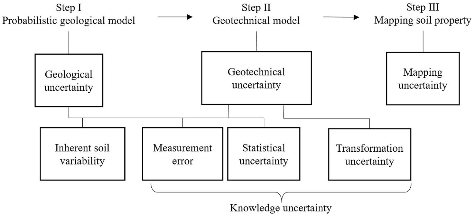
The methodology for developing a seismic microzonation map and the uncertainties at each step are presented in Figure 1. This methodology includes three major steps: (1) the development of probabilistic geological models, (2) the development of geotechnical models, and (3) the mapping of soil properties. Uncertainties must be considered for each step. Below, we explain the different uncertainties that affect each step, as well as the methodology used to quantify the uncertainties in the geological and geotechnical models and in the mapping of soil properties. Numerical examples are used to clarify the approach.

Figure 1.

Variabilities and uncertainties affecting seismic microzonation mapping.

Considered uncertainties

As illustrated in Figure 1, soil variability is primarily rooted in two sources of uncertainty: (1) uncertainty resulting from the inherent variability of the natural process and (2) knowledge-related uncertainties resulting from the statistical inference of a limited number of samples or from measurement imprecisions, that is, statistical uncertainty or measurement error (Wang et al., 2016). In addition, transformation uncertainty is introduced in the geotechnical variability when field or laboratory measurements are transformed into design soil properties using empirical or other correlation models (Phoon and Kulhawy, 1999; Wang et al., 2016). The propagation of the uncertainty to the design soil properties depends primarily on the combination of the analytical methods used and probabilistic analysis. Analytical methods vary from simple linear or empirical models to sophisticated constitutive models that include nonlinearity or elastoplasticity (Kaggwa and Kuo, 2011). Based on the complexity of the selected probabilistic and analytical methods, the response uncertainty varies from a single conventional statistical variance of averages to multiple probability density functions.

Geo-modeling: development of geological and geotechnical models

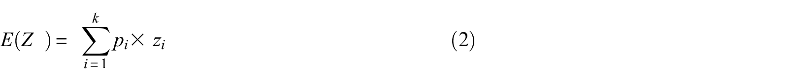
A quantitative geological model obtained by geostatistical simulation is presented, along with the probability of occurrence of the soil types. Probabilities are suggested to describe the different aspects of the uncertainty. The “simulation variance” is introduced as a quantitative measure of geological uncertainty (Salsabili et al., 2021; Yamamoto et al., 2014). Soil units are treated as Bernoulli variables with an outcome of either zero or one, and the variance $({\sigma }^2(x_i))$ is computed based on the discrete probability distribution of a random categorical variable $(x_i)$ with an event probability of $p_i$ (Equation 1 and Figure 2):

$${\sigma }^2(x_i)=p_i(1-p_i),x_i\in \{0,1\},i\in \{1,\dots ,k\}$$

(1)

Figure 2.

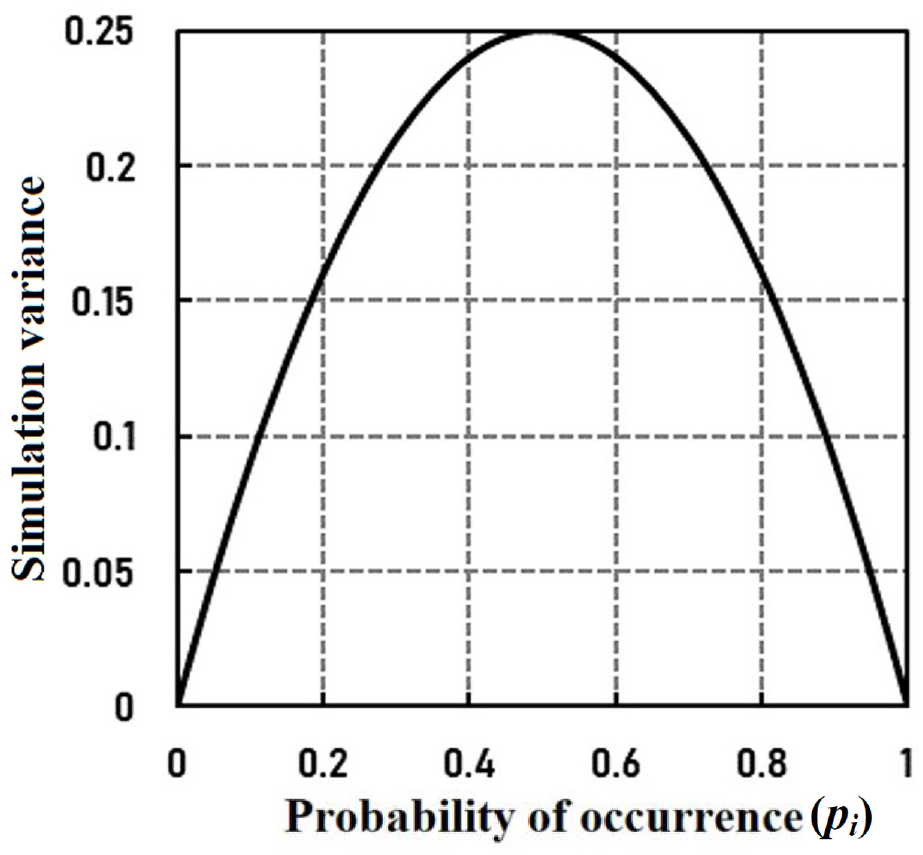
Simulation variance for a Bernoulli variable as a function of the probability of occurrence. When the probability of an outcome is close to 0 or 1, the variance (or uncertainty) is low, whereas when the probability is 0.5, the variance is maximal and equal to 0.25.

The flexibility of this approach is demonstrated in Figure 3, which shows an example of 2D grid cells of a binary soil unit (e.g. clay or sand). The certainty in distinguishing between the two soil units is represented by the probability of occurrence (Figure 3a). The values of 0 and 1 represent zones with sand or clay only. On the contrary, uncertain zones have probability values between 0 and 1; a probability of 0.5 conveys no information to distinguish the soil unit as either sand or clay and thus represents the maximum uncertainty. To develop the respective geotechnical model and its associated uncertainty, a deterministic or probabilistic interpretation of the geological model can be used. Figure 3b presents the deterministic interpretation of the geological model, in which the highest probability of occurrence is used to represent the soil type of the cells. The input geotechnical parameters are arbitrarily assumed to be

$$V_{s,sand}=400\mathrm{m/s},V_{s,clay}=200\mathrm{m/s},{\sigma }_{Vs,sand}^{}={\sigma }_{Vs,clay}^{}=40\mathrm{m/s}$$

It is clear that the local value on the V_s map varies sharply based on the cell’s soil type, whereas the ${\sigma }_{\mathrm{Vs}}$ map is uniform, with ${\sigma }_{Vs,sand}^{}={\sigma }_{Vs,clay}$ . The V_s map is determined solely by the binary variation of the soil units, not by the p_i values; difficulties arise in determining V_s when the probability is approximately 0.5. In the probabilistic approach, the mean $(E(Z))$ and combined variance $({\sigma }^2(Z))$ of a random geotechnical variable $(z_i)$ with a variance of ${\sigma }_{}^2(z_i)$ are determined using Equations 2 and 3:

$$E\left(Z_{}\right)=\sum _{i=1}^k{p}_i\times z_i$$

(2)

$${\sigma }^2\left(Z_{}\right)=\sum _{i=1}^k\left(p_i\times \left({\sigma }^2\left(z_i\right)+z_i^2\right)\right)-E{\left(Z_{}\right)}^2$$

(3)

For the example given in Figure 3, Equations 2 and 3 can be rewritten as follows:

$$V_s^{\mathrm{cell}}=p_{\mathrm{clay}}\times V_{s,\mathrm{clay}}+p_{\mathrm{sand}}\times V_{s,\mathrm{sand}}$$

(4)

$${\sigma }_{V_s^{\mathrm{cell}}}^2=(p_{\mathrm{clay}}\times ({\sigma }_{\mathrm{Vs},\mathrm{clay}}^2+V_{s,\mathrm{clay}}^2)+p_{\mathrm{sand}}\times ({\sigma }_{\mathrm{Vs},\mathrm{sand}}^2+V_{s,\mathrm{sand}}^2))-{\left(V_s^{\mathrm{cell}}\right)}^2$$

(5)

where $V_s^{\mathrm{cell}}$ and ${\sigma }_{V_s^{\mathrm{cell}}}^2$ are the mean and combined variance of an example grid cell with probabilities of occurrence of $p_{\mathrm{clay}}$ for clay and $p_{\mathrm{sand}}$ for sand. Figure 3c presents the probabilistic interpretation of the geological model. V_s and its associated variance values vary gradually based on the p_i values. The resulting variance $({\sigma }_{V_s^{\mathrm{cell}}}^2)$ considers the “combined variance” of both the geological and geotechnical variables, and the uncertainty of the geological model is also reflected in the V_s map. The uncertainty in V_s is lowest when the simulation variance is zero (i.e. when $p_i=1.0$ ) and highest when all members are equally probable (i.e. when $p_i=0.5$ ). This approach contributes to a more realistic model of V_s and its associated uncertainties. It also allows for an interpretation in the uncertain zone based on transitional or mixed soil units, for example, clayey sand or sandy clay, which is often referred to as a fuzzy interpretation in the spatial context (Wellmann and Regenauer-Lieb, 2012). Fuzziness is caused by imprecision and uncertainty, which are the main consequences of grouping similar soil units into broad categories with a certain level of ambiguity (McBratney and Odeh, 1997).

Figure 3.

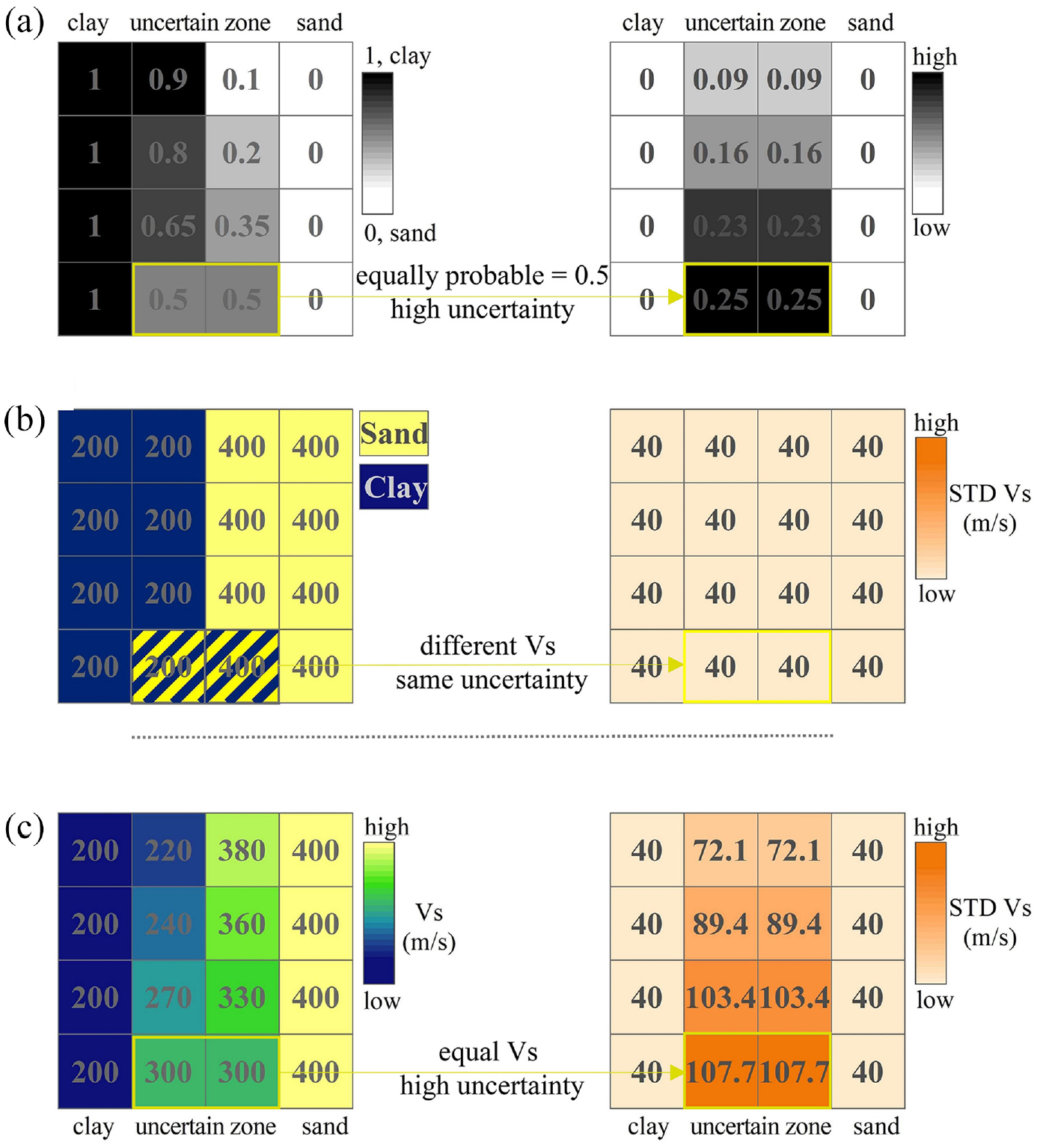
Numerical 2D grid cells presenting the methodology of probabilistic seismic mapping; (a) probability of possible outcomes for each soil unit in each cell and their visualized uncertainties (simulation variance); (b) deterministic V_s and uncertainty maps; (c) probabilistic V_s and uncertainty maps $V_{s,sand}=400\mathrm{m/s},V_{s,clay}=200\mathrm{m/s},{\sigma }_{Vs,sand}^{}={\sigma }_{Vs,clay}^{}=40\mathrm{m/s}$ .

Mapping of soil properties

In accordance with the evaluation of soil properties in 3D, a straightforward procedure for mapping local site conditions is the time-weighted averaging velocity of the vertically propagating shear wave through the column of blocks, as expressed by Equation 6. Figure 4 presents a schematic cross-section of the three dominant geologic layers in the Saguenay region (from top to bottom): postglacial soils, glacial deposits (till), and bedrock. For the postglacial soils, the V_s is considered a normal random variable with mean and variance, $V_{s,i}=N({\mu }_{\mathrm{Vs},i},{\sigma }_{\mathrm{Vs},i}^2)$ , for each block obtained by Equations 2 and 3. The glacial deposits are assumed to take normal random V_s values with constant mean and variance, $V_{s,\mathrm{till}}=N({\mu }_{\mathrm{Vs},\mathrm{till}},{\sigma }_{\mathrm{Vs},\mathrm{till}}^2)$ , whereas for bedrock, the V_s value is considered to be scalar. These assumptions are elaborated in the following sections.

Figure 4.

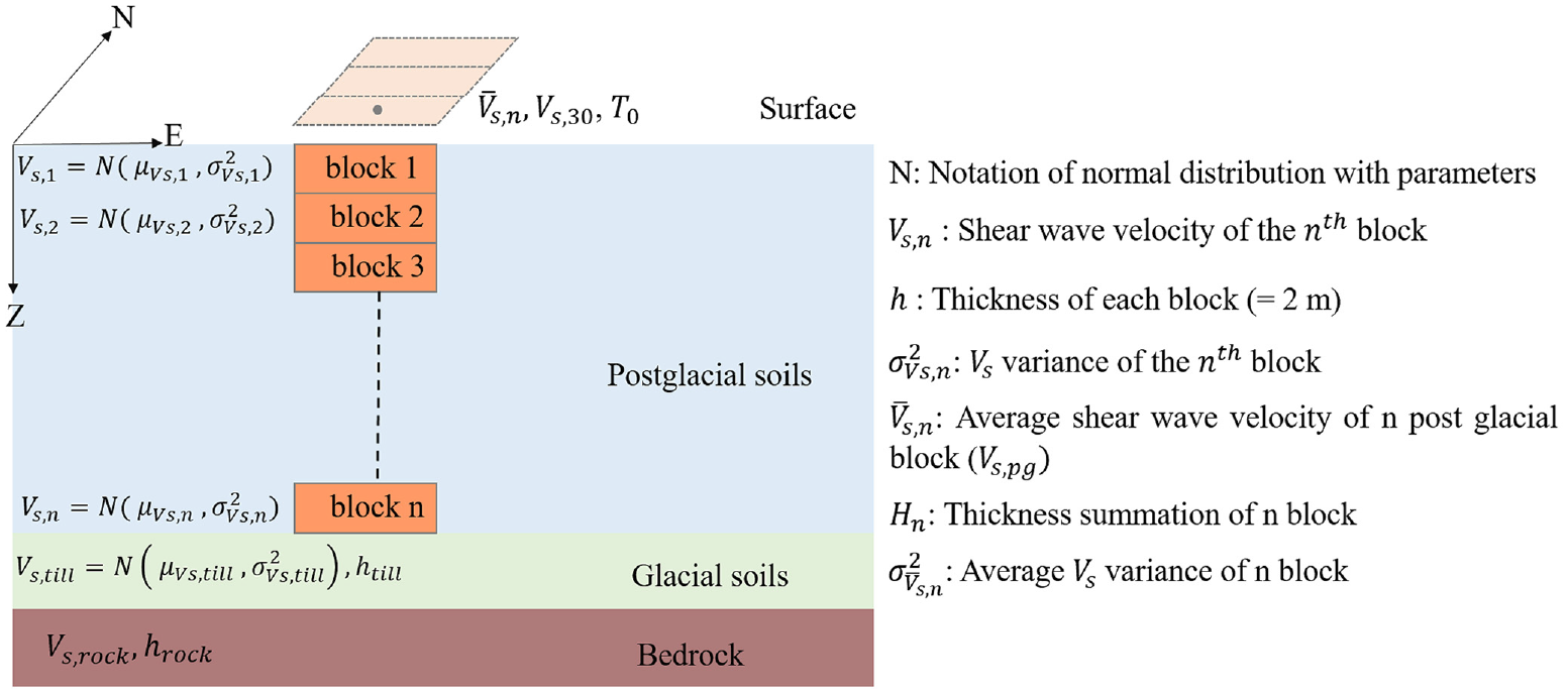
Schematic cross-section of a 3D model containing postglacial, glacial, and bedrock units.

For a given postglacial column with n blocks:

$$V_{s,\mathrm{pg}}={\overline{V}}_{s,n}=E[\frac{H_n}{\sum _{i=1}^n\frac{h}{V_{s,i}^{\}}}}]=\frac{H_n}{h}\times E\left[\frac{1}{\sum _{i=1}^n\frac{1}{V_{s,i}}}\right]$$

(6)

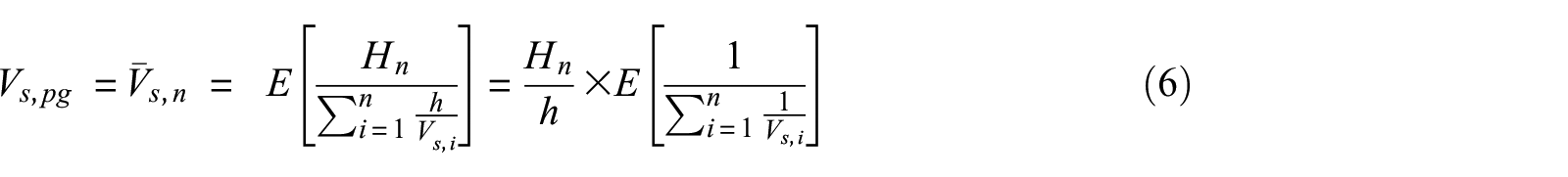
where the thickness h of each block is assumed to be 2 m and the total thickness is $H_n$ . The parameters H_n and h are not random variables but the $V_{s,i}$ is a random variable. Therefore, to estimate the shear-wave velocity profiles $({\overline{V}}_{s,n})$ , one should rely on stochastic Monte Carlo simulations and develop a set of $V_{s,i}$ realizations. In this regard, a problem could arise when the random variable $V_s$ tends toward zero, $1/V_s$ tends toward infinity, and the average of $1/V_s$ becomes unstable. However, in practice, the $V_s$ values are all well above zero and this problem does not arise. One solution would be to assume that $V_s$ in each block follows a lognormal distribution. Hence, given that $C.V.={\sigma }_{\mathrm{Vs}}^2/{\mu }_{\mathrm{Vs}}$ is quite small, the fit of lognormal and normal laws are almost equivalent.

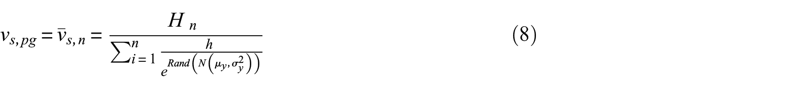
Considering Y =  $\ln (V_s)$ , ${\mu }_y$ and ${\sigma }_y^2$ are equal to the mean and variance of Y, respectively. The relations between the mean and variance in real and log space are expressed as follows:

$${\mu }_y=\ln {\mu }_{\mathrm{Vs}}-\frac{{\sigma }_y^2}{2}$$

(7a)

$${\sigma }_y^2=\ln (\frac{{\sigma }_{\mathrm{Vs}}^2}{{\mu }_{\mathrm{Vs}}^2}+1)$$

(7b)

Therefore, for one realization of the random normal distribution of ${\overline{v}}_{s,n}$ , Equation 6 can be rewritten as Equation 8:

$$v_{s,pg}={\overline{v}}_{s,n}=\frac{H_n}{{\sum }_{i=1}^n\frac{h_{}}{e^{Rand\left(N\left({\mu }_y,{\sigma }_y^2\right)\right)}}}$$

(8)

Saguenay city study area

Saguenay city was selected as the study area due to its relatively high seismic hazard (https://earthquakescanada.nrcan.gc.ca/) and the presence of heterogeneous Quaternary sediments with complex spatial and vertical architecture. It is the largest municipality within the Saguenayã Lac-Saint-Jean region, covering 1136 km² with a population of 147,100. The recent most important seismic event was the 1988 M 6.0 Saguenay earthquake. The epicenter of the earthquake, which had a mid-crustal depth of 29 km, was 35 km south of the downtown area (Du Berger et al., 1991). The earthquake’s secondary effects included soil liquefaction, rock falls, and landslides observed within a 200 km radius of the epicenter (Lamontagne, 2002).

The bedrock in the Saguenay region is part of the Grenville province of the Canadian Shield, which is composed mainly of crystalline Precambrian rocks (Davidson, 1998). Based on the surficial geology maps, cross-sections, and subsurface data (CERM-PACES, 2013; Daigneault et al., 2011; LaSalle and Tremblay, 1978), the soil deposits can be grouped into four major categories: till, gravel, clay, and sand (Figure 5).

• Till: This glacial sediment is located at the base of the stratigraphic soil column; it is compact and semiconsolidated. Till is the most common soil unit in the study area, with thicknesses ranging from a few meters to >10 m at certain locations. With the exception of rock outcrops, till covers the bedrock elsewhere, which is an important assumption in the 3D modeling approach.

• Gravel: This coarse sediment is mainly of glaciofluvial and alluvial origin; it consists of gravel, sand, and occasionally till. This unit occurs infrequently in the region and is often in contact with till, sand, or clay units.

• Clays: These fine postglacial sediments are the most abundant soil type by volume in the study area. Clays are classified as silt, silty clay, or clay. They generally have a thickness of up to 10 m and may attain a maximum thickness of >100 m in the lowlands.

• Sand: This group consists mainly of coarse glaciomarine deltaic and prodeltaic sediments, as well as alluvial sands composed of sand and gravely sand.

Other unconsolidated sediments, such as loose postglacial sediments (alluvium, floodplain sediments, organic sediments, and so on.) and landslide colluvium, can also be found in minor proportions. For the purposes of this study, these unconsolidated sediments are classified as sand, clay, and/or gravel based on grain size.

Figure 5.

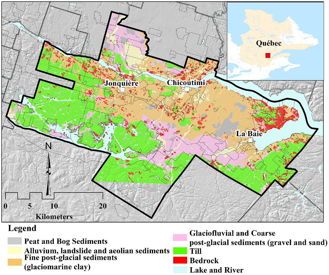
Saguenay city study area: surficial geology map (modified from Daigneault et al., 2011).

3D probabilistic geological modeling

Geostatistical simulation is widely used to model the spatial architecture of major lithofacies in reservoir and mineral resource modeling (Deutsch, 2006; Pyrcz and Deutsch, 2014). Sequential indicator simulation (SIS) represents a practical approach for cases without an obvious genetic shape that can be incorporated into object-based modeling. It makes use of indicator kriging (IK), in which the Monte Carlo simulation draws a precise category at each location (Deutsch, 2006). SIS was used to determine the spatial boundaries of categorical variables (in this case, clay, sand, and gravel) and to develop a model that captures the heterogeneity of soil properties prior to estimating geotechnical parameters (Salsabili et al., 2021). The geostatistical simulation requires a full 3D volume to determine the soil type of the glacial and postglacial deposits. Accordingly, the entire model space was subdivided into a raster with equal cell sizes (also referred to as voxels or blocks representing the smallest unit of a given soil type). Salsabili et al. (2021) developed the model on the basis of comprehensive datasets, including 3524 borehole logs, 26 geological cross-sections, and 973 virtual boreholes. They were combined to create the total soil and till thickness maps and to generate the bedrock topography. The space between the top and bottom of each interface was filled with 75 m × 75 m × 2 m blocks to perform the geostatistical simulation. Then, the 3D model of soil type was created by using SIS. The spatial statistics of a target variable were reproduced with a set of alternative models of categorical variable spatial distributions called realizations (Deutsch and Journel, 1997). The method consists of three steps, which are as follows:

1. Transformation of the soil types into K indicator variables:

   $$i(u_{\alpha };k)=\{\begin{array}{c}1\mathrm{if}\mathrm{category}k\mathrm{prevails}\mathrm{at}\mathrm{location}u,k=1,\dots ,K.\hfill \\ \multicolumn{1}{c}{0\mathrm{otherwise}}\end{array}$$
   (9)

2. Determination of indicator variograms to model the spatial continuity of the indicator soil types (see Supplemental Appendix);

3. Sequential and reproducible simulations of the soil types based on field observations (conditional simulation).

Overall, 100 realizations were generated using the conditional SIS method to determine the probability of occurrence (p_i) for each of the postglacial deposits: clay, sand, and gravel. The resulting probability values were used to estimate the associated simulation variance (uncertainty). Figures 6 and 7 show the probabilistic interpretations of the plan and the cross-section of the 100 SIS realizations in a typical area containing all four surficial soil units.

Figure 6.

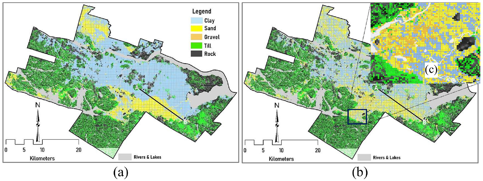
Map of (a) soil units with the highest probability of occurrence at the ground surface and (b) one SIS realization showing sand, clay and gravel. (c) Local blown-up showing the surface soil variability in the SIS map.

Figure 7.

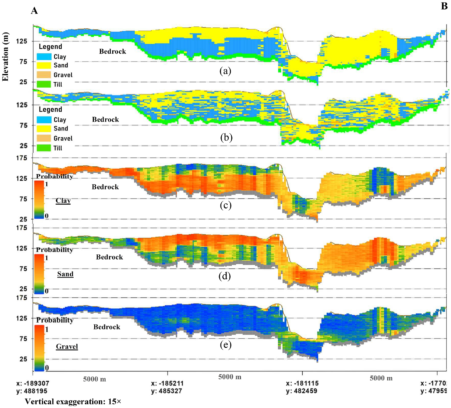
Stratigraphic cross-sections A–B: (a) soil units with the highest probability of occurrence; (b) one SIS realization of sand, clay, and gravel. Individual probabilities of occurrence for (c) clay, (d) sand, and (e) gravel obtained from a set of 100 conditional SIS realizations.

Development of the 3D geotechnical model

For practical convenience and because the term “geotechnical model” has different meanings in the literature related to stability analysis (Phoon and Tang, 2019), the geotechnical model considered in this article is valid within the limits of elastoplastic behavior before ultimate failure. In this context, the geotechnical model was created similarly to the 3D geologic model in terms of engineering parameters, that is V_s. The procedure includes two main steps: (1) developing V_s empirical correlations and (2) creating a 3D V_s model that incorporates the probabilistic geologic model and V_s empirical correlations.

V_s empirical correlations

In situ V_s measurements can be obtained by invasive methods, such as cross-hole or downhole drilling, as well as noninvasive methods, such as refraction or surface wave methods (Hunter and Crow, 2012; Garofalo et al., 2016a, 2016b). The seismic piezocone penetration test (SCPTu) is an invasive method that provides optimized V_s intervals and continuous penetration results, allowing the development of reliable empirical correlations between V_s and strength-based soil parameters. In addition, cone penetration test (CPT) profiling provides continuous logs of the interpreted soil stratigraphy (Prins and Andresen, 2021). Interpretations are based on the values of the CPTu parameters, such as the cone tip resistance (q_t), sleeve friction and friction ratio in former studies (Robertson and Campanella, 1983) and the normalized cone resistance and friction in later studies (Robertson, 2009, 2016). For the development of V_s empirical correlations, we (1) perform SCPTu field tests, (2) collect and store existing data in a database, (3) develop CPTu-V_s correlations by using the results of 15 SCPTu surveys, and (4) estimate V_s on the basis of CPT and standard penetration test (SPT) SPT data by using empirical correlations for the entire study area. The final step involves developing V_s-depth correlations to assist in determination of the 3D V_s values.

Field testing program

Fifteen SCPTu surveys were carried out using a standard type 2 piezocone with the following specifications: 60°apex angle, 10 cm² conical tip base area, and 150 cm² sleeve area, with the filter located at the shoulder. A dual-array seismic cone mounted on the top of the piezocone allows the measurement of arriving vertically propagating seismic body waves. For a given depth, the SCPTu method generates four types of data: V_s, the raw cone tip resistance q_c, the frictional cone resistance f_s, and the penetration pore pressure u₂. The field program followed principally the ASTM Designation Standard (D5778-12) (2012) procedure and preprocessing, and corrections were done in accordance with Lunne et al. (2002) and Robertson (2009). SCPTu surveys were performed at the penetration rate of 2 cm/s. High-resolution CPTu data were collected every 1 cm, and V_s values were recorded at every 50 cm depth interval. Shear-wave velocities were determined from seismic signals by applying the cross-correlation algorithm (Campanella and Stewart, 1992). The cone tip was corrected, and q_c and f_s were cross-correlated by using the software CPeT-IT (GeoLogismiki, 2014). The predrill depth was assessed by applying the geological 3D model (Salsabili et al., 2021) prior to performing the field test. The maximum depth of testing was set to 30 m. The termination conditions were reached at the bedrock contact or in the presence of very stiff soil, such as till or gravel, where the pushing force reached the maximum. The ground water table in saturated drained soils (e.g. sands) was identified on the basis of pore water pressure (u₀∼u₂) and that in clayey soils was determined through dissipation tests. In some cases, before the sounding hole was destroyed, a piezometer was installed to measure the piezometric level. Precautions were taken in soils above the groundwater table that were saturated due to capillarity.

Database

The collected database contains more than 700 soil samples that were tested under laboratory conditions for physical properties such as unit weight, permeability, natural water content, Atterberg limits, plasticity, and liquidity index, as well as for mechanical properties such as preconsolidation stress, compression index, and sensitivity. The results show a relatively high variability of the sensitivity of the fine-grained sediments, ranging from 1 to ∼2700; however, most of the data vary from 1 to 50, with a median value of 44. The natural water content (w) ranges from 9% to 70%; most of the plasticity index data vary from 5% to 25%; more than 50% of the samples have a liquidity index greater than one; and the unit weights range between 17 and 19 kN/m³, with an average value of approximately 18 kN/m³ and a relatively weak correlation between the unit weight and depth (R² ≈ 0.2).

In situ tests with invasive methods were conducted during three field campaigns (Figure 8):

• Fifteen recent SCPTu surveys were conducted by the Université du Québec à Chicoutimi (UQAC) research group. The data include the complete set of q_t, f_s, u₂, and V_s measurements.

• Ninety-one CPT profiles were obtained during the 1980s and 1990s by the Quebec Ministry of Transport (MTQ). The CPT data set is limited to measurements of q_c and f_s. For the purposes of the present study, the field reports were digitalized, and V_s was calculated using the developed sit-specific CPT-V_s correlation.

• Sixty-four standard penetration tests (SPTs) were acquired during the 1980s and 1990s by the MTQ. The results were incorporated in the determination of the geotechnical properties of coarse-grained soils.

Figure 8.

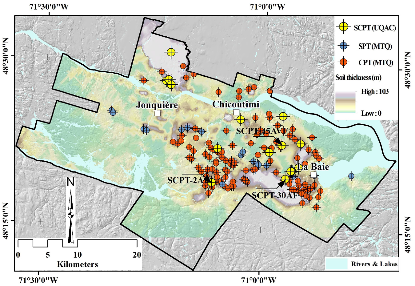
Distribution of geotechnical test sites. The background presents soil thickness (modified from Salsabili et al., 2021), and validation was conducted at the three indicated sites.

Development of CPTu-V_s correlation

After performing 15 SCPTu surveys and collecting raw data, the data were statistically preprocessed due to the presence of surface noise. As part of the process, the V_s outliers were determined using a box plot, in which their values were above the upper quartile or below the lower quartile of 1.5 times the interquartile range. Next, 568 CPTu-V_s data pairs were retained for analysis. The V_s values were assumed to be consistent for the intervals of 50 cm, and the midpoint of each interval was assumed to be the depth (D) of the measured V_s. Figure 9 shows the relationships between V_s and the CPTu-based parameters. The color range is based on the variation in the soil behavior type index (I_c). The positive correlation between the CPTu measurements and V_s was mainly attributed to the soil’s stiffness properties and overburden pressure, which were represented by q_t and D, respectively.

Figure 9.

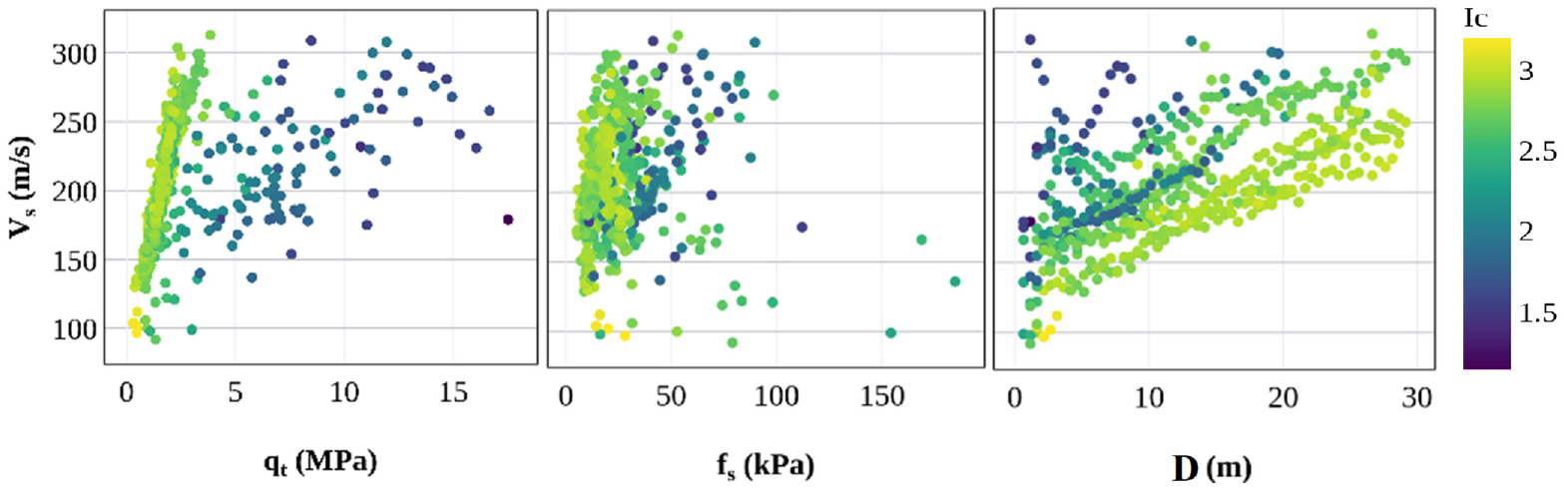
Relationships between V_s and CPTu-based parameters. q_t is the corrected cone tip resistance in MPa, f_s is the sleeve friction resistance in kPa, and D is the depth (m).

The general CPTu-V_s correlation was developed for postglacial soils using 568 data pairs (Equation 10). By distinguishing between cohesive (clay-like) and cohesionless (sand-like) soils, simple and robust regression equations for non-piezocone profiles can be developed. The soil behavior type index (I_c) was used to classify soil into two categories: clay (I_c > 2.6) and sand (I_c < 2.6). The soil-specific CPT-V_s correlations for the clayey soil (Equation 11) and for the sandy soil (Equation 12) are indicated as follows:

$$\mathrm{All}\mathrm{soils}:V_s=7.648q_t^{0.35}{I}_c^{0.322}{D}^{0.031}(1+B_q{)}^{0.653}N=568R^2=0.692$$

(10)

$$\mathrm{Clay}:V_s=10.052q_t^{0.379}{D}^{0.085}N=453R^2=0.813$$

(11)

$$\mathrm{Sand}:V_s=38.757q_t^{0.174}{D}^{0.099}N=115R^2=0.545$$

(12)

where q_t is in kPa, D is depth (m), and B_q is normalized pore pressure (for detailed calculation see Robertson, 2009).

V _s-depth profile

The V_s-depth profile is of interest because it is frequently used as a proxy for V_s prediction (Motazedian et al., 2011, 2020; Nastev et al., 2016a; Rosset et al., 2015). The depth (D) has a significant correlation with the measured V_s value and enables straightforward prediction of the spatial variability of V_s by assigning different depth values.

Following the retrieval and processing of the older MTQ CPT logs, 4600 averaged data pairs of q_t and f_s were generated at 50 cm intervals. The V_s values were predicted by using the developed empirical CPT-V_s correlations (Equations 11 and 12) for sands and clays. In addition, the SPT data were converted into V_s by applying the empirical relationship of Ohta and Goto (1978) for gravel sediments. Then, linear and nonlinear V_s-depth regression analyses were conducted on SCPTu and CPT-V_s data for sand and clay soils (Equations 13 to 15) and on SPT-V_s data for gravels (Equation 16). The results are also shown in Figure 10. The standard deviations of the V_s-depth correlations were used as a measure of statistical uncertainty. Note that the data from CPT-Vs and particularly SPT-V_s were subjected to epistemic uncertainties. These sources of uncertainty have not been considered in our methodology, due to the limitations in analytical calculations. The use of site-specific V_s correlations for the dominant soil types of the study area (sand and clay) is, however, intended to reduce the epistemic uncertainties:

$$\mathrm{Sand}\mathrm{and}\mathrm{Clay}\mathrm{mixture}:V_s=144.9+2.55\times D{\sigma }_{\mathrm{Vs},\mathrm{SC}}=34\mathrm{m}/\mathrm{s}{R}^2=0.43$$

(13)

$$\mathrm{Clay}:V_s=114.5+9.4\times D^{0.76}{\sigma }_{\mathrm{Vs},\mathrm{clay}}=33\mathrm{m}/\mathrm{s}{R}^2=0.59$$

(14)

$$\mathrm{Sand}:V_s=150.47\times D^{0.149}{\sigma }_{\mathrm{Vs},\mathrm{sand}}=21\mathrm{m}/\mathrm{s}{R}^2=0.66$$

(15)

$$\mathrm{Gravel}:V_s=46.86+61.55\times D^{0.50}{\sigma }_{\mathrm{Vs},\mathrm{gravel}}=34\mathrm{m}/\mathrm{s}{R}^2=0.52$$

(16)

Figure 10.

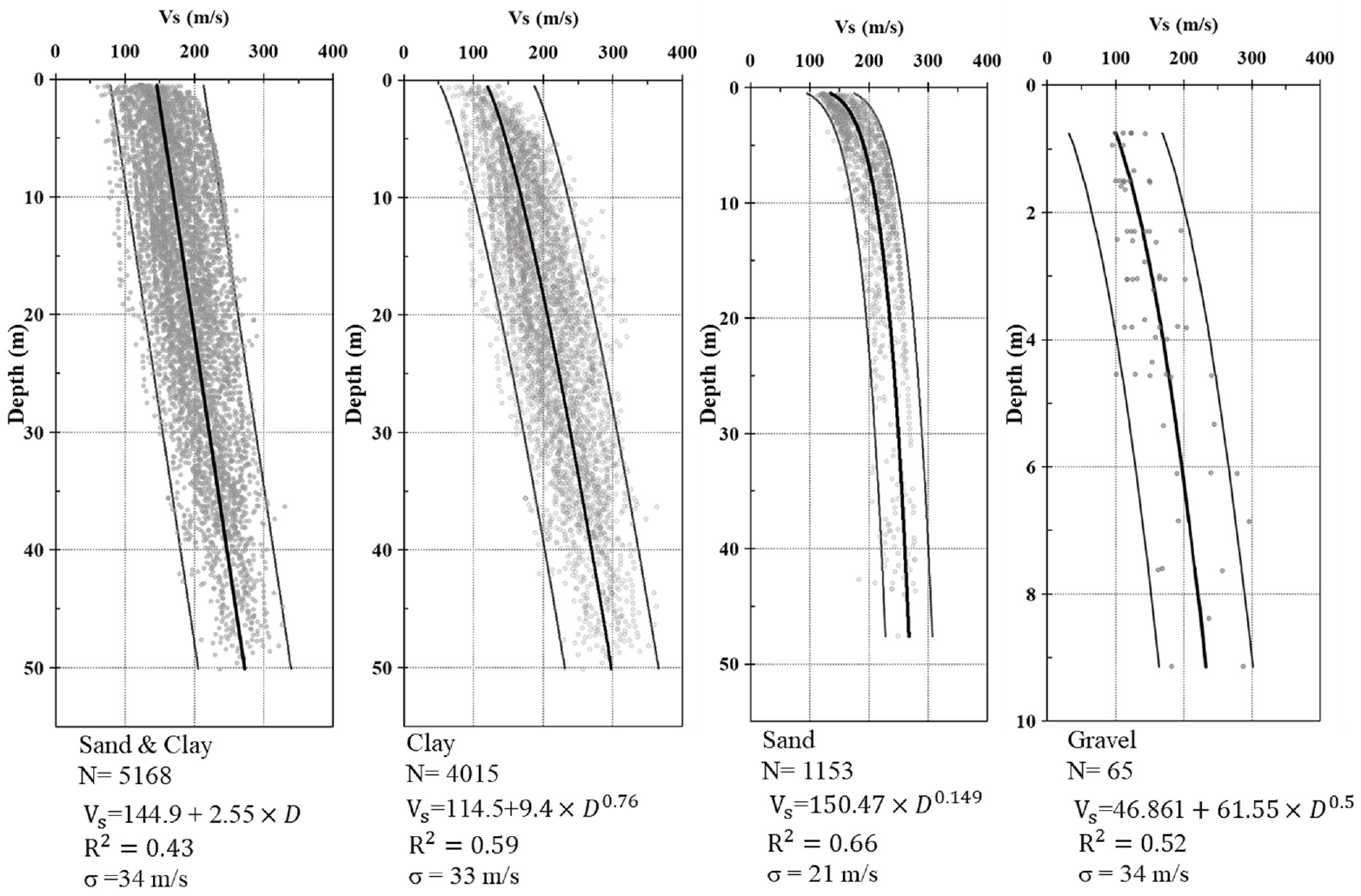
Interval V_s-depth relationships for postglacial sandy and clayey soils.

3D geotechnical modeling

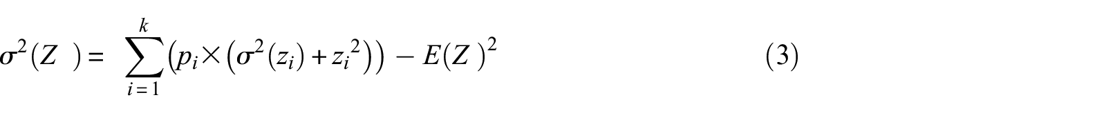
A probabilistic method was used to estimate Vs. The V_s values for postglacial deposits were estimated on the basis of the probabilistic approach by using Equation 2. The V_s values were calculated by using the V_s-depth profiles (Equations 14 to 16) and the probability of soil occurrence (p_i). Then, the associated uncertainty was calculated on the basis of the combined variance approach (Equation 3) where the variance of the regression models for each soil type was incorporated for each block. Given that regression analysis removes the trend from the observed data, it allows residuals to behave as independent variables with a normal distribution, indicating that the V_s of each block is assumed to be normal. Figure 11a presents the developed 3D geotechnical model, which indicates the spatial distribution of V_s, and its associated uncertainty is shown in Figure 11b. It should be mentioned that the spatial correlation of the shear wave velocity within each geological unit is overlooked in this approach (see Toro (2022), auto-regressive model). This limitation can be addressed in a future study by consideration of V_s a random field variable using a geostatistical approach by V_s profiling (Passeri et al., 2020); full 3D modeling, such as sequential Gaussian simulation (Pyrcz and Deutsch, 2014); or with Markov chain Monte Carlo simulations (Wang et al., 2016).

Due to the lack of V_s measurements in glacial deposits and bedrock and the geological similarities between till and crystalline bedrock, the regional V_s values of the glacial deposits and bedrock were calculated from the data obtained by Motazedian et al. (2011) (V_{s, till} = 580 m/s and σ_{Vs, till} = 175 m/s) and Nastev et al. (2016b) (V_{s, rock} = 2500 m/s).

Figure 11.

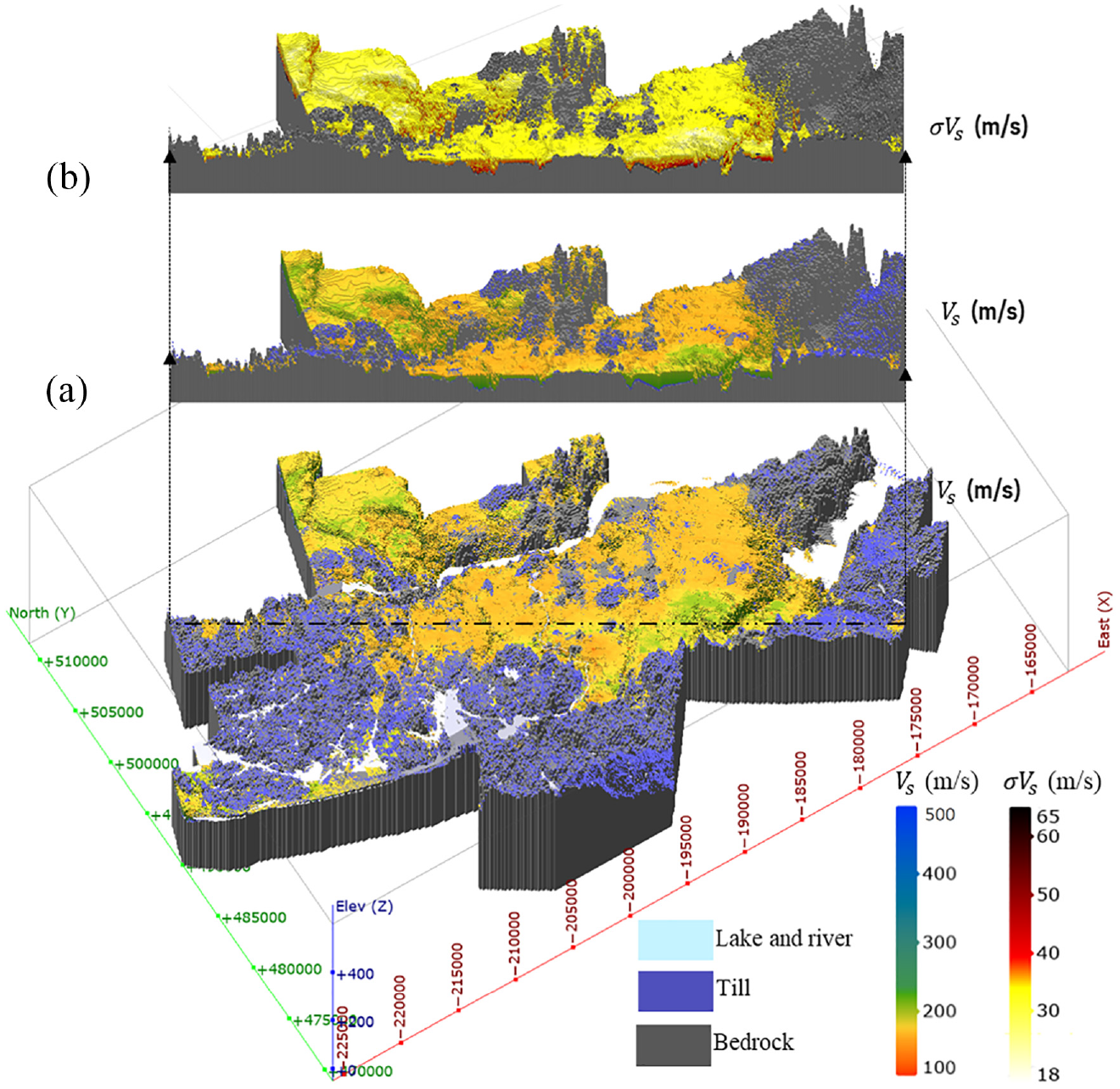
Probabilistic geotechnical model for the city of Saguenay: (a) 3D shear-wave velocity and (b) associated V_s standard deviation.

Comparison to recorded data

Three sites (Figure 8) composed of (1) sensitive clay soils, (2) transitional soil layers, and (3) sandy soils with thin interbeds of clays were selected to visually demonstrate the capability and efficiency of the developed probabilistic and deterministic models in predicting the V_s values of the various soil types. In general, the predicted V_s values correspond fairly well to the measured values, although several inconsistencies were noted.

Soil classification was first performed using widely accepted CPTu-based charts and indices to determine the soil stratigraphy in selected SCPTu locations (Robertson, 2009, 2016). The normalized soil behavior type (SBTn) chart proposed by Robertson (2016) delineated the in situ behavior of soils, such as sensitivity, contractivity, or tendency to dilate, in addition to textural descriptions. Figure 12a shows a dominant fine-grained soil profile with alternating soft clay and silty clay sediment layers known as sensitive clays. Lower values of q_t and f_s and higher values of u₂ are typical indicators for distinguishing these soils. The CPTu parameters (q_t, f_s, and u₂) fluctuate continuously over a short distance before stabilizing with depth, confirming the continuous stratigraphy of Laflamme-sensitive clays. Figure 12b depicts heterogeneous transitional soils with alternating clay and silty clay soils. The profile starts with interbedded thin (<10 cm) sandy soils that transform into fairly soft transitional soils, most likely silty clay and clay soils. Figure 12c depicts a site with clean sandy soil interspersed with thin interbeds of fine-grained silt and clay soils. The variation in CPTu parameters indicates a sharp rather than a transitional change in soil behavior type.

Figure 12.

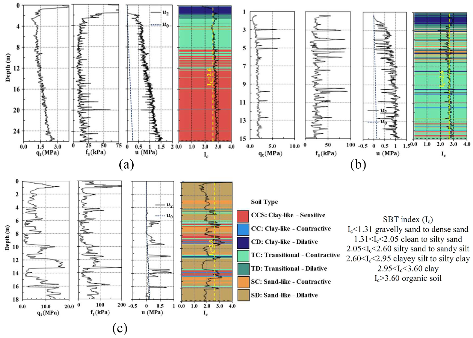
SCPTu profiles at three different sites composed of (a) sensitive clay soils, (b) transitional soil layers, and (c) sandy soils with thin interbeds of clay; classification based on the SBTn chart (Robertson, 2016).

Figure 13 shows cross-sections of the 3D V_s block model and their associated standard deviations at the three representative SCPTu locations. Equation 2 was calculated for each 3D block to generate the probabilistic V_s model $V_s^p$ (Figure 13a). The respective standard deviations obtained from the combined variance (Equation 3) are illustrated in Figure 13b. As indicated earlier, the soil type behavior at these locations varies from top to bottom as follows: clayey, transitional, and sandy soil. The resulting $V_s^p$ values depend primarily on the depth and the probabilities of occurrence of the soil types. Based on Equation 3, the resulting ${\sigma }_{V_s^p}$ values represent a combined standard deviation of $V_{s,\mathrm{clay}}$ , $V_{s,\mathrm{sand}}$ , and $V_{s,\mathrm{gravel}}$ , with their respective probabilities incorporated. The relatively higher ${\sigma }_{V_s^p}$ values for the sandy soil profile (Figure 13b bottom) than for the clayey soil (Figure 13b top) were attributed to higher heterogeneity in the sand profile, which resulted in higher simulation variance.

Figure 13.

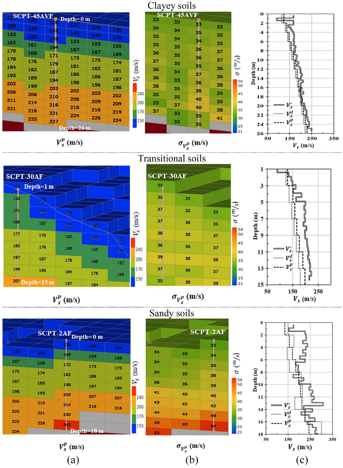
(a) Probabilistic 3D V_s block model and (b) associated standard deviations at the three different sites (from top to bottom): clayey, transitional, and sandy soil; (c) comparison of the respective V_s profiles: SCPTu measurements $(V_s^{*})$ , deterministic predictions $(V_s^d)$ , and probabilistic predictions $(V_s^p)$ .

Figure 13c compares the measured V_s values using the SCPTu test, V_s predictions based on the deterministic $V_s^d$ approach, and V_s predictions based on the probabilistic $V_s^p$ approach. The deterministic $V_s^d$ values depend only on the depth of occurrence of each soil type, which are, respectively, shown in Equations 14 to 16. Essentially, the prediction methods serve as a good proxy for V_s measurements. In clays, which make up the majority of the study area, the estimated V_s values correspond closely to their measured counterparts. In transitional soils, we observed underestimations, but interestingly, the probabilistic approach provided better results. In sandy soils, due to intrinsic heterogeneity, the measured V_s values fluctuate considerably, and both the deterministic and probabilistic approaches underestimated V_s; however, in clay interbeds, the estimated V_s values were in good agreement with the measured values. We should note that the comparison of the model to recorded shear wave velocity profiles at three locations is insufficient for a general statement. Additional analyses with a larger dataset by performing non-invasive geophysical tests are needed to make general statements about the performance of the model.

V_s, ₃₀ and T₀ mapping

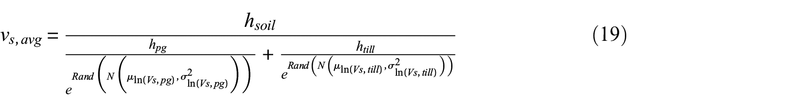
Seismic site parameters, namely the shear-wave velocity of the top 30 m, $V_{s,30}$ , and the fundamental site period, T₀, were introduced to conduct site classifications. The computations were performed based on a 2D raster with a cell size of 75 m × 75 m. The time-averaged shear-wave velocity was first estimated using Monte Carlo simulations of 20,000 realizations for postglacial soils from the ground surface down to the interface with the underlying glacial soils or bedrock (Equation 8). Then, the averaged V_S values of a complete geologic soil column, including the postglacial soils, till, and rock, were obtained by performing Monte Carlo simulations of 20,000 realizations, as, respectively, indicated in Equations 17, 18, and 18 (the optimum number of realizations can be found in Supplemental Appendix B):

$$v_{s,30}=\frac{30}{\frac{h_{\mathrm{pg}}}{e^{\mathrm{Rand}\left(N({\mu }_{\ln (\mathrm{Vs},\mathrm{pg})},{\sigma }_{\ln (\mathrm{Vs},\mathrm{pg})}^2)\right)}}+\frac{h_{\mathrm{till}}}{e^{\mathrm{Rand}\left(N({\mu }_{\ln (\mathrm{Vs},\mathrm{till})},{\sigma }_{\ln (\mathrm{Vs},\mathrm{till})}^2)\right)}}+\frac{(30-h_{\mathrm{soil}})}{V_{s,\mathrm{rock}}}}$$

(17)

$$T_0=\frac{4\times h_{\mathrm{soil}}}{V_{s,\mathrm{avg}}}$$

(18)

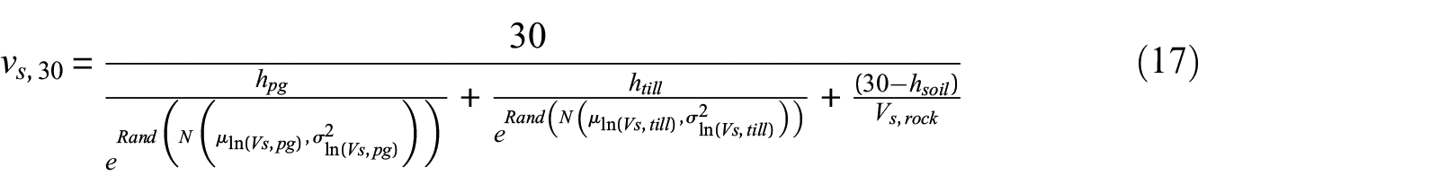
where N is the notation of normal distribution with parameters; $V_{s,\mathrm{pg}}$ , $V_{s,\mathrm{till}}(=N(580\mathrm{m}/\mathrm{s},{175}^2))$ , and $V_{s,\mathrm{rock}}(=2500\mathrm{m}/\mathrm{s})$ are the shear-wave velocities of postglacial, glacial deposits, and bedrock, respectively; $V_{s,\mathrm{pg}}$ is computed using Equation 6 with the incorporation of the 3D V_s model; $h_{\mathrm{soil}}=h_{\mathrm{pg}}+h_{\mathrm{till}}$ ; and $V_{s,\mathrm{avg}}$ is the soil average shear-wave velocity obtained by Equation 19:

$$v_{s,\mathrm{avg}}=\frac{h_{\mathrm{soil}}}{\frac{h_{\mathrm{pg}}}{e^{\mathrm{Rand}\left(N({\mu }_{\ln (\mathrm{Vs},\mathrm{pg})},{\sigma }_{\ln (\mathrm{Vs},\mathrm{pg})}^2)\right)}}+\frac{h_{\mathrm{till}}}{e^{\mathrm{Rand}\left(N({\mu }_{\ln (\mathrm{Vs},\mathrm{till})},{\sigma }_{\ln (\mathrm{Vs},\mathrm{till})}^2)\right)}}}$$

(19)

The final maps of the seismic site parameters are shown in Figure 14. At first glance, the spatial distribution of the seismic site parameters appears to follow the general variation patterns of surficial soil thickness (Figure 8). In shallow areas, where the thickness of the overlying soils is less than 30 m, $V_{s,30}$ and T₀ exhibit the same pattern. The majority of the region was classified as rock or very stiff soil sites, with an average vibration period of less than 0.2 s, indicating that the seismic site response at these locations coincides at high frequencies, similar to rock outcrops (Zhao et al., 2006). In contrast, regions with thicker sediments, where $V_{s,30}$  < 360 m/s and T₀ > 0.4 s, represent sites with seismic responses that resemble medium and soft soil behavior during seismic incidents. These zones will generally be sensitive to distant strong earthquakes with dominant low-frequency signals.

Figure 14.

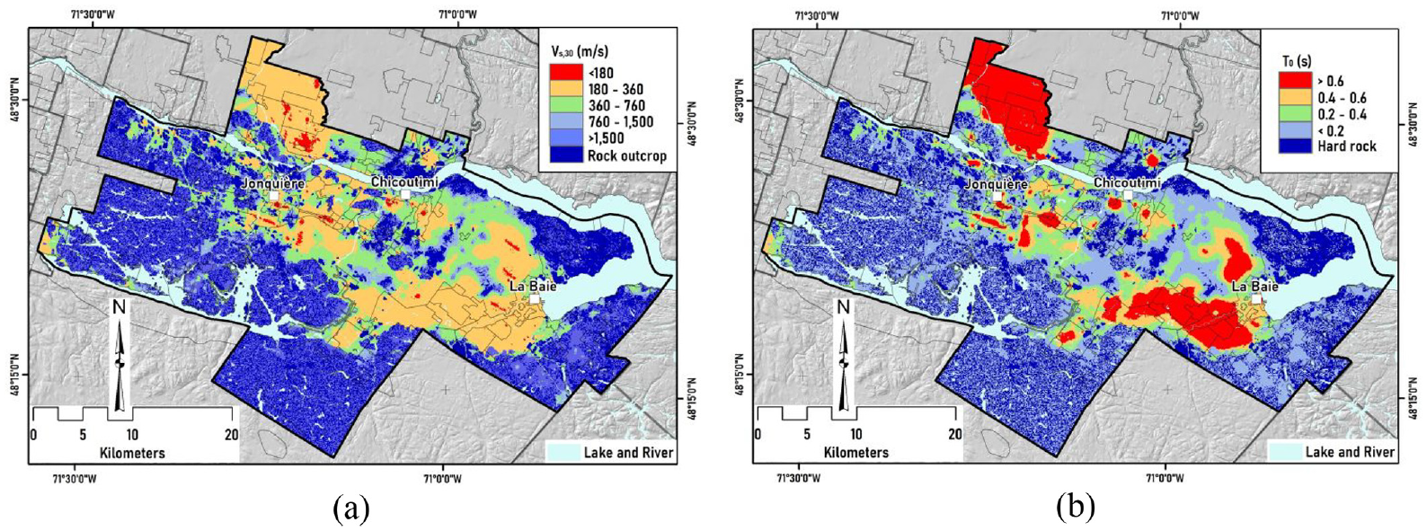
Spatial distributions of (a) $V_{s,30}$ and (b) fundamental site period, $T_0$ .

As a result of the Monte Carlo simulations, the uncertainties associated with the seismic site parameters V_s,₃₀ and T₀ can also be determined. The ${\sigma }_{V_{s,30}}$ and ${\sigma }_{T_0}$ values were determined by resampling the 20,000 simulations for the complete soil column.

It should be noted that in this study, ${\sigma }_{\mathrm{Vs},\mathrm{rock}}^2$ was neglected to better reflect the uncertainty of only soil deposits. The spatial distributions of ${\sigma }_{V_{s,30}}$ and ${\sigma }_{T_0}$ are shown in Figure 15a and b.

Figure 15.

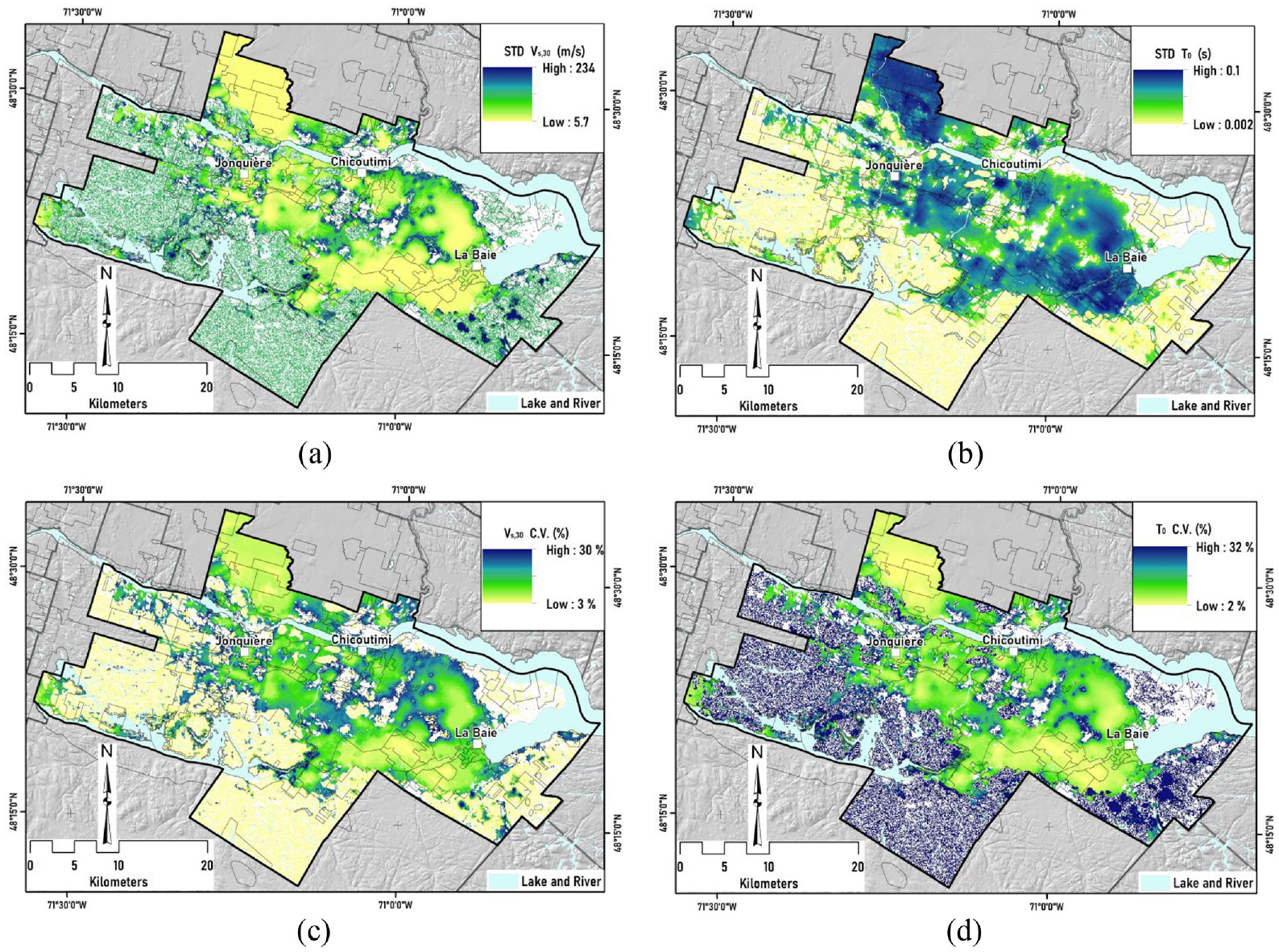
Spatial distributions of the associated uncertainties of seismic site parameters: (a) ${\sigma }_{V_{s,30}}$ , (b) ${\sigma }_{T_0}$ , (c) V_s,₃₀ coefficient of variation, and (d) T₀ coefficient of variation.

Visual comparisons of Figure 15a and b with the corresponding spatial distributions in Figure 14 indicate that the uncertainties are approximately proportional to the modeled $V_{s,30}$ and T₀ values. Therefore, the distribution of ${\sigma }_{V_{s,30}}$ showed an approximately inverse spatial pattern relative to that of ${\sigma }_{T_0}$ . Figure 15c and d presents the coefficients of variation of $V_{s,30}$ and T₀, respectively. The areas with relatively high uncertainty in $V_{s,30}$ and T₀ are characterized by shallow deposits.

The standard deviations shown in Figure 15 represent the model uncertainties that result from both the spatial variation of the geological soil units and the predicted V_s data. The efficiency of the developed methodology can be observed in Figure 16, which depicts the effect of geological uncertainty on the resulting geotechnical model. The certainty of the geological model is highest (p_i∼ 1) in the vicinity of the boreholes, and thus, the combined uncertainty of the geological and geotechnical models has its lowest value at these locations. In contrast, as the distance from the boreholes increases, the spatial uncertainty in the prediction of the soil units increases, leading to increased geotechnical model and seismic map uncertainty.

Figure 16.

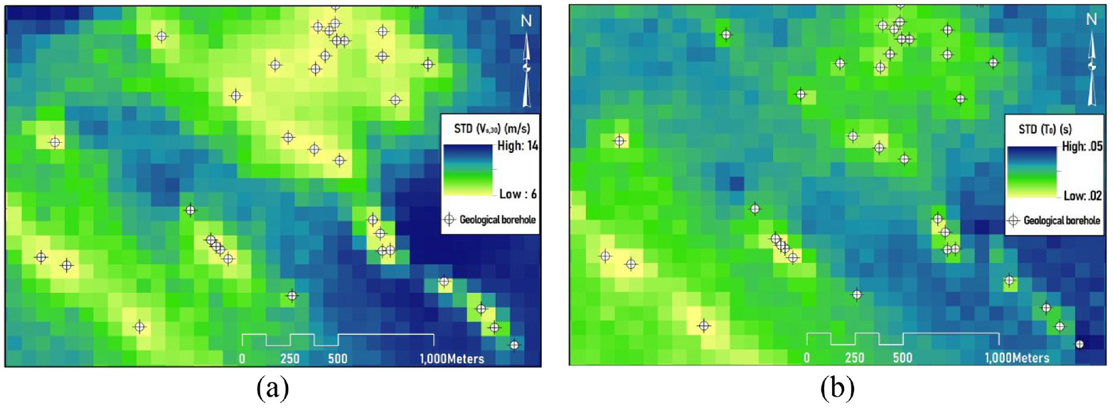
The effects of geological spatial uncertainty on the uncertainties of seismic site parameters: (a) ${\sigma }_{V_{s,30}}$ and (b) ${\sigma }_{T_0}$ .

Conclusion

This study proposed a novel approach for determining the spatial uncertainties of the geological model and propagating these uncertainties to the geotechnical response variable V_s. A probabilistic approach for seismic site characterization was introduced to develop the 3D V_s model and to assess the uncertainty associated with combining various types of uncertainties in building the geological and geotechnical models. The model uncertainty was calculated using the combined variance of the probabilistic geological model and the variance of the V_s-depth regression model.

Given the complex stratigraphic setting and soil type heterogeneity of the study area, SIS was used to predict the probability of occurrence of the postglacial soil deposits. To quantify the uncertainty associated with the geological model, a method for determining the simulation variance was introduced.

Due to the lack of direct V_s measurements, it was necessary to supplement the V_s values inferred from existing CPT logs, which covered most of the study area. SCPT surveys were conducted to develop empirical site-specific CPT-V_s correlations for postglacial sediments in the study area, thereby reducing the epistemic uncertainties associated with the use of existing global correlations.

The V_s correlation functions were developed using nonlinear regression analyses, which incorporated q_t, depth, and the SBT indicators for general soil types. In soil-specific correlations, the depth and q_t control the significant variability of V_s, and the developed CPT-V_s correlations were proposed for clay-like and sand-like soils.

The final output consisted of maps of the main site effect parameters V_s,₃₀ and T₀, the uncertainties of which were assessed by using a 3D V_s model. The V_s,₃₀ and T₀ spatial distributions appear to follow the general variation patterns of the surficial soil thickness. In shallow sediments, the $V_{s,30}$ and T₀ maps represent rock or very stiff soil conditions, with seismic responses in short vibration periods ≤0.2 s. In contrast, regions with thicker sediments denote sites with potential responses that resemble medium to soft soil conditions, with longer vibration periods dominating.

The respective ${\sigma }_{V_{s,30}}$ and ${\sigma }_{T_0}$ maps represent the inherent random and epistemic uncertainty in the models, which are associated with both the spatial variability of the geological units and the statistical dispersion of the V_s data. As a result, the combined uncertainty of the geological and geotechnical models decreases in the vicinity of the geological boreholes due to the higher certainty of the geological model. In contrast, as the distance from the boreholes increases, the spatial uncertainty increases, resulting in greater uncertainties of V_s,₃₀ and T₀.

Supplemental Material

sj-pdf-1-eqs-10.1177_87552930221132576 – Supplemental material for Probabilistic approach for seismic microzonation integrating 3D geological and geotechnical uncertainty

Supplemental material, sj-pdf-1-eqs-10.1177_87552930221132576 for Probabilistic approach for seismic microzonation integrating 3D geological and geotechnical uncertainty by Mohammad Salsabili, Ali Saeidi, Alain Rouleau and Miroslav Nastev in Earthquake Spectra