Sage Journals: Discover world-class research

Abstract

One-dimensional (1D) site response analysis (SRA), which considers vertically propagating seismic waves from the bedrock to the surface, has been a common technique among geotechnical engineers to examine site-specific ground shaking. However, observations from past earthquakes and analytical studies indicate that idealizations ingrained in 1D SRA may be too severe to capture the ground truth, such as the omissions of spatial variability of soil properties, surface topography, and basin and directivity effects. Physics-based three-dimensional ground motion simulations (GMSs) can incorporate these factors and yield more reliable predictions. In this study, we utilize ground motions from 57 physics-based broadband (from 0 to 8–12 Hz) GMS for a region of Istanbul. A total of 2912 sites with experimentally measured soil profiles that are distributed over the 30 km-by-12.5 km area are also modeled as soil columns and analyzed through 1D SRA. The ground responses from 1D SRA and three-dimensional (3D) GMS are then compared for all 57 earthquake scenarios. These systematic comparisons are then used for examining model features that are correlated with variations in the ratios of various ground motion intensity measures (IMs) and for developing regression-based formulas that can be used for determining simple factors for the considered region to correctly scale (up or down) the site-specific ground motion intensities obtained from 1D SRA, including peak ground acceleration (PGA), peak ground velocity (PGV), and spectral acceleration (S_a) values.

Keywords

Physics-based ground motion simulations regional-scale analysis 3D versus 1D site response analysis site amplification site classification

Introduction

Site response analysis (SRA), especially one-dimensional (1D), has been commonly adopted as a simple numerical technique for geotechnical engineers to assess the potential ground-shaking level and evaluate the seismic hazard at a specific location (Kramer, 1996). 1D SRA is designed to simulate the seismic waves (e.g. P- or S-wave or both) traveling vertically from a certain depth (usually bedrock), through different horizontal soil layers, and eventually to the ground surface. This analysis method can consider the local soil conditions and hence calculate the time histories, ground response spectra, and other intensity measures (IMs), such as peak ground acceleration (PGA) and peak ground velocity (PGV), and characterize site amplification factors (Rathje et al., 2010). The usage of 1D SRA is versatile, including ground motion characterization (Huang and Mccallen, 2023; Stewart et al., 2002), seismic hazard assessment (Abrahamson, 2006; Baker et al., 2021), soil liquefaction evaluation (Idriss and Boulanger, 2008), site-specific design (Bradley, 2015), soil–structure interaction (Stewart et al., 1999; Zhang et al., 2022), and so on.

Despite the aforementioned advantages, 1D SRA also has some obvious drawbacks. Various studies and observations have demonstrated that 1D SRA cannot accurately capture (1) the soil profile and ground motion spatial variability (Madiai et al., 2016; Makra and Chávez-García, 2016; Pretell et al., 2022) and basin effects (McGann et al., 2021); (2) topographic site-effect amplification/de-amplification (Bahrampouri and Rodriguez-Marek, 2023; Smerzini et al., 2011); and (3) impact of incident angles of seismic waves and wave scattering (de la Torre et al., 2022; Oral et al., 2022). Formulations and mechanisms of 1D SRA have inevitably limited its capability to consider these factors. To remedy this, three-dimensional (3D) physics-based ground motion simulation (GMS), embedded with a realistic kinematic rupture model, 3D soil velocity structure and surface topography, can intrinsically take all the source-path-site effects into account.

3D physics–based GMS is pretty computationally expensive, and the minimum shear wave velocity and maximum resolvable frequency are two major factors controlling its accuracy, applicability, and computational cost (Poursartip et al., 2020). A relatively high minimum shear wave velocity cannot capture the ground motion amplification due to soft soil layers in the shallow crust. At the same time, a low maximum resolvable frequency will directly filter out the high-frequency components in seismic waves, which are crucial for some ground motion IMs, such as PGA and short-period S_a. Up to date, a number of 3D GMS have been carried out to simulate earthquakes in different regions, for example, Istanbul, Turkey (Akinci et al., 2017; Douglas and Aochi, 2016; Infantino et al., 2020; Zhang et al., 2023, 2021), San Francisco, USA (McCallen et al., 2021), Bogota, Colombia (Riaño et al., 2021), Tangshan, China (Fu et al., 2017), Southern California, USA (Graves, 1998; Lee et al., 2008; Roten et al., 2016), Tokyo, Japan (Ichimura et al., 2015), Grenoble, France (Stupazzini et al., 2009), Norcia, Italy (Pitarka et al., 2022), and Kobe, Japan (Pitarka et al., 1998). Most of the existing 3D GMS have a lower than 2 Hz maximum frequency or a high frequency but with only a limited number of earthquake scenarios (e.g. $< = 5$ ), which are hence unable to consider the uncertainty in ground motions.

Furthermore, few studies have quantitatively compared the performance between 3D GMS and 1D SRA. Olsen et al. (2000) conducted a 3D 2-Hz wave propagation simulation for an M_w 4.9 earthquake in Southern California and then assessed the capability of 1D models to predict the surface response. Smerzini et al. (2011) built a 3D model with a homogeneous basin embedded in a layered soil media to simulate an M_w 6.0 earthquake in Central Italy and compared it with 1D models. Özcebe et al. (2019) utilized 3D, two-dimensional (2D), and 1D approaches to evaluate the seismic site amplification of the Norcia basin when subjected to the M_w 6.5 2016 earthquake. All these studies indicated that the 1D simulations were inclined to underpredict motions. A particular study from Seylabi et al. (2021) performed a nonlinear 3D physics–based GMS up to 5 Hz for Garner Valley in Southern California and also used the computed motions from 3D GMS at the bedrock level to conduct 1D SRAs for 3640 stations. However, their study showed inconsistency in the findings with respect to PGA—that is, 1D simulations yielded greater PGAs than 3D.

In this study, we utilize simulated ground motions from 57 physics-based broadband (from 0 to 8–12 Hz) GMS for the Istanbul region in Turkey (Zhang et al., 2023, 2021). A total of 2912 sites distributed over a 30 km by 12.5 km area with measured soil profiles are modeled as 1D soil columns and then analyzed by performing 1D SRA on OpenSees (Mazzoni et al., 2006). In all 57 3D GMSs, the acceleration time histories at both ground surface and engineering bedrock¹ levels of those 2912 boreholes were recorded. Thus, the bedrock-level motions are adopted as the input motions in 1D SRA. Then, the ground surface responses from 1D SRA are compared with ones computed from 3D GMS for all 57 earthquake scenarios.

A comprehensive comparison is conducted between 3D and 1D simulations. We first examine the 3D/1D ratios of mean horizontal and vertical PGA, PGV, and S_a in multiple periods among 57 scenarios and the frequency distributions and their uncertainties of those ratios over 2912 sites. Then, we investigate correlations between 3D/1D ratios and three commonly used parameters—that is, $V_{s} 30$ , mean curvature (a topographical index), and bedrock depth. Finally, 12 representative stations are selected, and their complete S_a curves (0.01–10 s) are compared. Our results are consistent with the literature. Although de-amplifications may occur, most sites (>90%) have larger responses in 3D GMS compared to 1D SRA, with mean amplification factors of 1.4 and 1.3, for PGA and PGV, respectively. Also, these ratios are largely correlated with bedrock depth while loosely related with $V_{s} 30$ and mean curvature. Overall, such systematic comparisons can significantly help us quantitatively understand the relative importance of each factor controlling the performance of 1D SRA, the uncertainty of 1D SRA for different IMs, and the conditions in which 1D SRA can deliver accurate results and vice versa. The computed ratios can also be used to improve the performance of 1D SRA for the Istanbul region.

Problem background

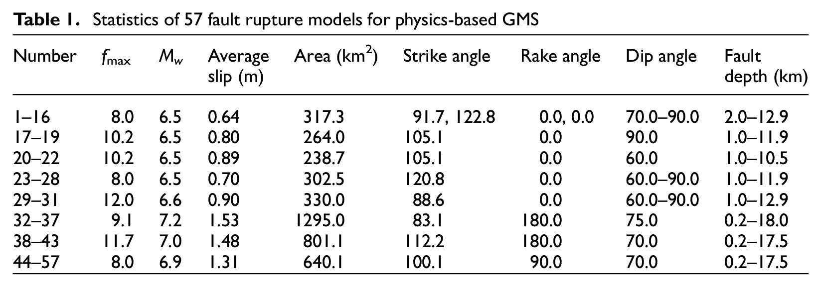
Recently, we performed 57 3D broadband (from 0 to 8–12 Hz) physics-based GMS for a region in Istanbul, Turkey (Zhang et al., 2023) using Hercules (Tu et al., 2006). These 57 GMS, which included realistic surface topography and ocean bathymetry, 3D heterogeneous soil media, and source models with varying earthquake magnitudes (M_w = 6.5–7.2), locations of hypocenters, fault geometry, and rupture time distributions aimed at generating numerous possible strong earthquakes from the North Anatolian faults. Table 1 summarizes some key parameters for fault rupture models. Figure 1 shows the topography/bathymetry map and locations of fault planes and hypocenters for the studied area. The domain of interest (i.e. the red rectangle in the upper center area) encompasses a 30 km by 12.5 km region, in which a total of 2912 borehole stations were drilled from a completed microzonation study (LessLoss Integrated Project, 2004–2007). These boreholes were approximately evenly distributed in every 250 m in both north–south and east–west directions, and standard penetration tests (SPTs) were conducted to measure all boreholes’ properties including soil layer thickness, shear wave velocity $(V_{s})$ , compressional wave velocity $(V_{p})$ , and density for each layer (OYO, 2007). Figure 2 displays the average $V_{s}$ for the upper 30-m depth $(V_{s} 30)$ and bedrock depth for all 2912 boreholes within the domain of interest. As seen, 2276, 632, and 4 boreholes belong to site classes D, C, and B, respectively (NHERP, 2015).

Table 1.

Statistics of 57 fault rupture models for physics-based GMS

Number	f _max	M_w	Average slip (m)	Area (km²)	Strike angle	Rake angle	Dip angle	Fault depth (km)
1–16	8.0	6.5	0.64	317.3	91.7, 122.8	0.0, 0.0	70.0–90.0	2.0–12.9
17–19	10.2	6.5	0.80	264.0	105.1	0.0	90.0	1.0–11.9
20–22	10.2	6.5	0.89	238.7	105.1	0.0	60.0	1.0–10.5
23–28	8.0	6.5	0.70	302.5	120.8	0.0	60.0–90.0	1.0–11.9
29–31	12.0	6.6	0.90	330.0	88.6	0.0	60.0–90.0	1.0–12.9
32–37	9.1	7.2	1.53	1295.0	83.1	180.0	75.0	0.2–18.0
38–43	11.7	7.0	1.48	801.1	112.2	180.0	70.0	0.2–17.5
44–57	8.0	6.9	1.31	640.1	100.1	90.0	70.0	0.2–17.5

Figure 1.

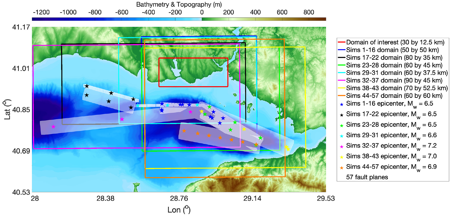
Topography/bathymetry map, dimensions, and locations of fault ruptures of all 57 simulations.

Figure 2.

$V_{s} 30$ (left) and bedrock depth (right) for the domain of interest. Square dots represent the according locations of 2912 boreholes.

In every 3D physics–based GMS, we recorded the three-directional (east-west, north-south, and up-down) acceleration time histories at both ground surface and engineering bedrock levels of all 2912 boreholes. The time histories at the bedrock levels are used as excitations for the following 1D SRA, which will be explained in the next section.

1D SRA

Each borehole station contains a different soil profile. Thus, we built a total of 2912 1D soil columns in OpenSees (Mazzoni et al., 2006). Figure 3 illustrates the configurations of the 1D soil column model built in OpenSees for 1D SRA. As seen, three dashpots are attached to the bottom of the soil column, and the equivalent nodal forces are applied to the other ends of the dashpots. Here, all nodal force time histories have a uniform duration of 30 s and a time increment of 0.01 s. The soil materials and layers in 1D SRA are identical to those in 3D GMS. Eventually, 2912 × 57 ≈ 1666 k 1D SRA are conducted using OpenSeesMP on the supercomputer Frontera at the Texas Advanced Computing Center (TACC) (Stanzione et al., 2020). Acceleration time histories in all three directions at the surface level are recorded.

Figure 3.

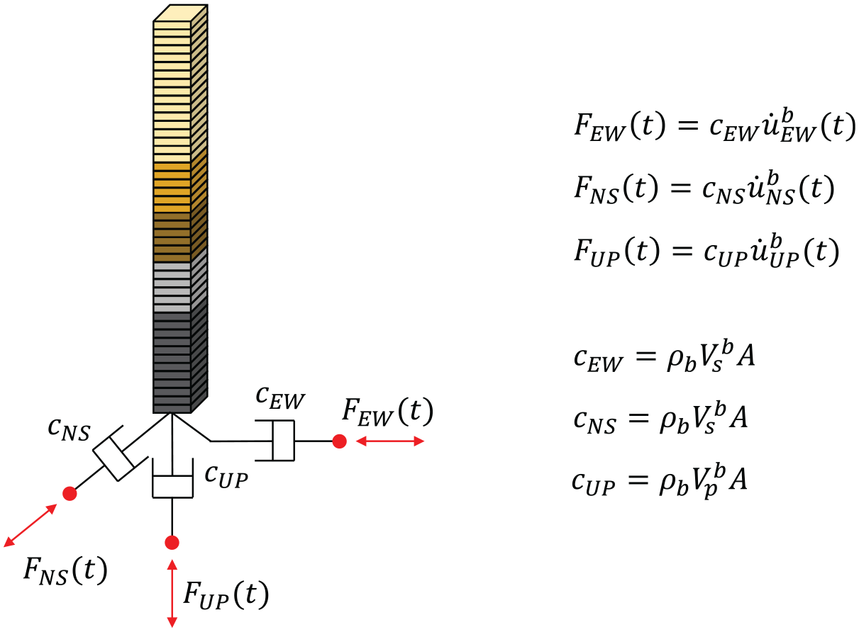
Configurations of the 1D soil column model built in OpenSees for 1D SRA. $ρ_{b}$ , $V_{s}^{b}$ , and $V_{p}^{b}$ denote the density, shear, and compressional wave velocity of the underlying bedrock, respectively. Here, we adopt a very large $V_{s}^{b} (5000 m / s)$ to mimic a rigid base boundary condition. A is the area of the horizontal surface of the brick element, which is always 0.1 m × 0.1 m = 0.01 m² in this study. ${\overset{\cdot}{u}}_{EW}^{b}$ , ${\overset{\cdot}{u}}_{NS}^{b}$ , and ${\overset{\cdot}{u}}_{UP}^{b}$ represent the computed velocity time histories at the bedrock level in E-W, N-S, and UP directions from 3D physics–based GMS, respectively.

1D SRA versus 3D GMS

PGA

This section compares computed horizontal (in the format of RotD50) and vertical PGAs ratios of 3D GMS to 1D SRA. Figure 4 shows average ratios of PGAs among all 57 earthquake simulations for the entire region, and Figure 5 displays their distributions and other statistical properties, including the mean, median, and standard deviation. As seen, most sites experience amplified responses under 3D simulations—that is, 92% and 89% for horizontal and vertical PGAs, respectively. And the ratios range from 0.5 to 2.5, with a mean amplification factor of 1.37. The majority of sites that exhibit de-amplified behavior are located at the edges of the domain or land, which is because we (1) assumed a simplified multi-layer soil media outside the domain due to lack of data and (2) modeled the ocean as viscoelastic solid since Hercules is not yet able to simulate the fluid–solid coupling behavior. Such assumptions may lead to less reliable results for 3D GMS (Zhang et al., 2023).

Figure 4.

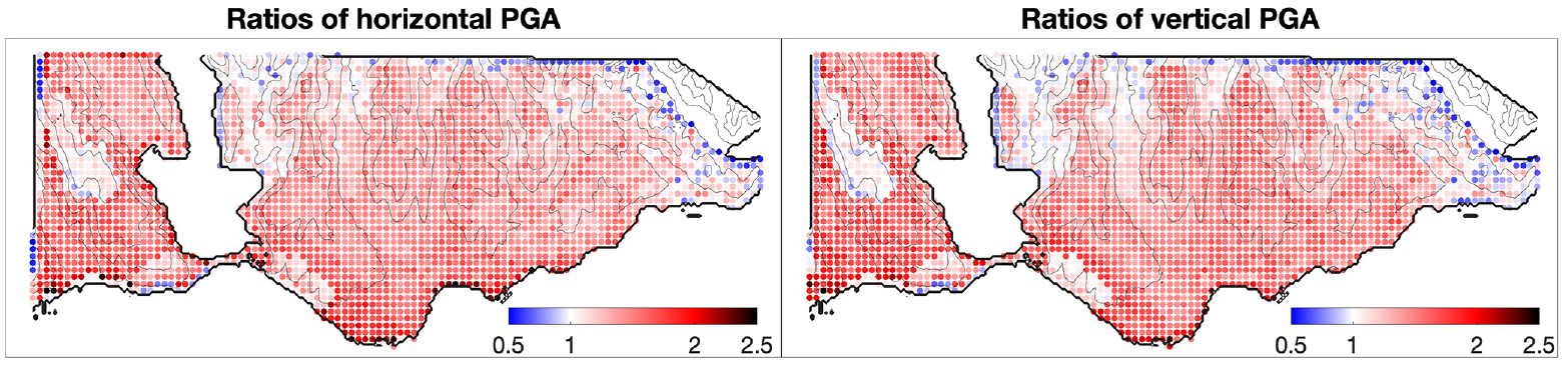
Horizontal (left) and vertical (right) PGA ratios of 3D GMS to 1D SRA.

Figure 5.

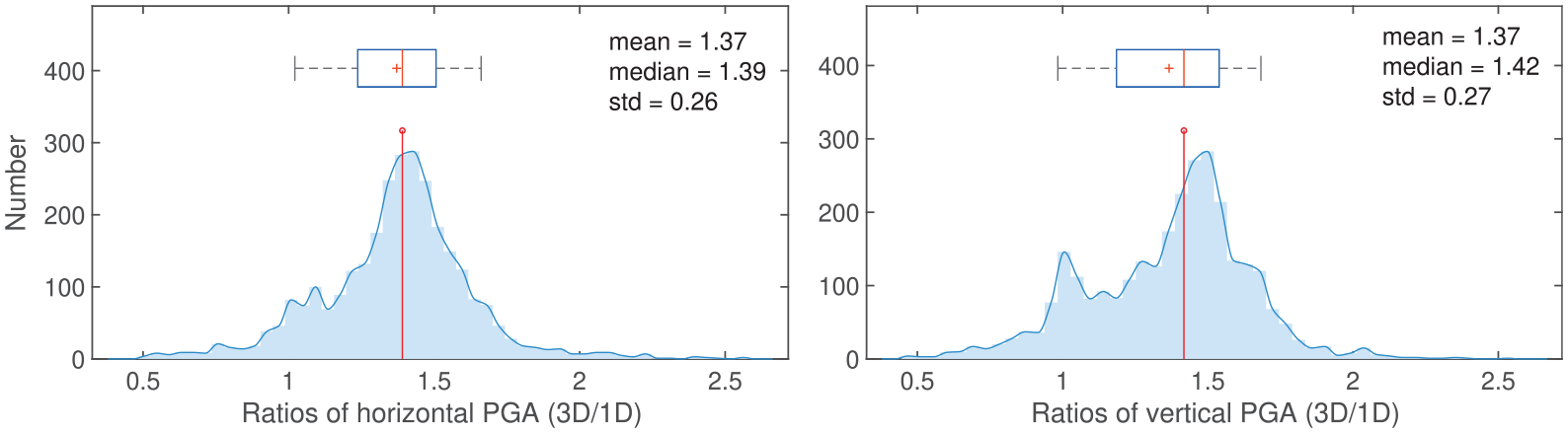
Distributions of horizontal (left) and vertical (right) PGA ratios of 3D GMS to 1D SRA. The vertical red line and cross symbol indicate the median and mean ratios, respectively.

PGV

Similarly, we compare both horizontal and vertical PGVs from 3D GMS and 1D SRA. Compared to PGA, PGV is more accurate in predicting the response of long-period structures, such as pipelines and bridges (Zhang et al., 2020). As shown in Figure 6, similar to PGA ratios, most sites’ PGVs are intensified when 3D effects are considered (91% and 85% for horizontal and vertical PGVs, respectively). Figure 7 examines the distributions of PGV ratios. As seen, compared to PGAs, PGV ratios are slightly reduced—that is, from 1.39 to 1.31 and 1.42 to 1.26 for their median values in horizontal and vertical directions, respectively. This phenomenon indicates that the 3D effects have a larger impact on PGAs than PGVs.

Figure 6.

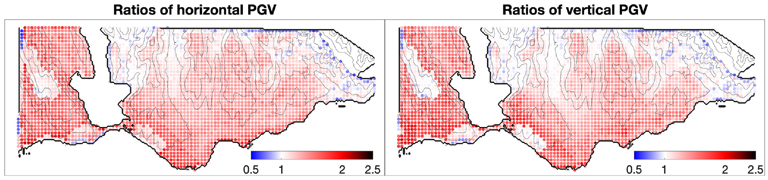
Horizontal (left) and vertical (right) PGV ratios of 3D GMS to 1D SRA.

Figure 7.

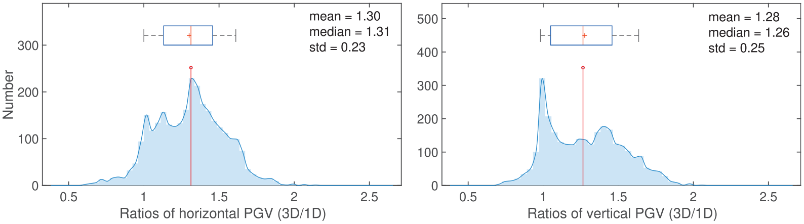
Distributions of horizontal (left) and vertical (right) PGV ratios of 3D GMS to 1D SRA. The vertical red line and cross symbol indicate the median and mean ratios, respectively.

Spectral acceleration (S_A)

This section investigates the ratios of horizontal S_as at six different periods, including 0.1, 0.2, 0.5, 1, 5, and 10 s. Figures 8 and 9 show the S_a ratios for the entire domain of interest and their statistical distributions among all 2912 sites, respectively. It can be seen that although the majority of sites’S_as are amplified at all six periods under 3D simulations, the maximum and minimum values of S_a ratios are bi-polarized at the periods ranging from 0.5 to 1.0 s. In other words, the variances of S_a ratios increase. In addition, an average amplification factor of 1.35∼1.40 is observed for periods below 1.4 s, while gradually reduced to 1 when the period increases. Similar to both PGA and PGV, most sites that have de-amplified responses are located at the domain edges or on shorelines.

Figure 8.

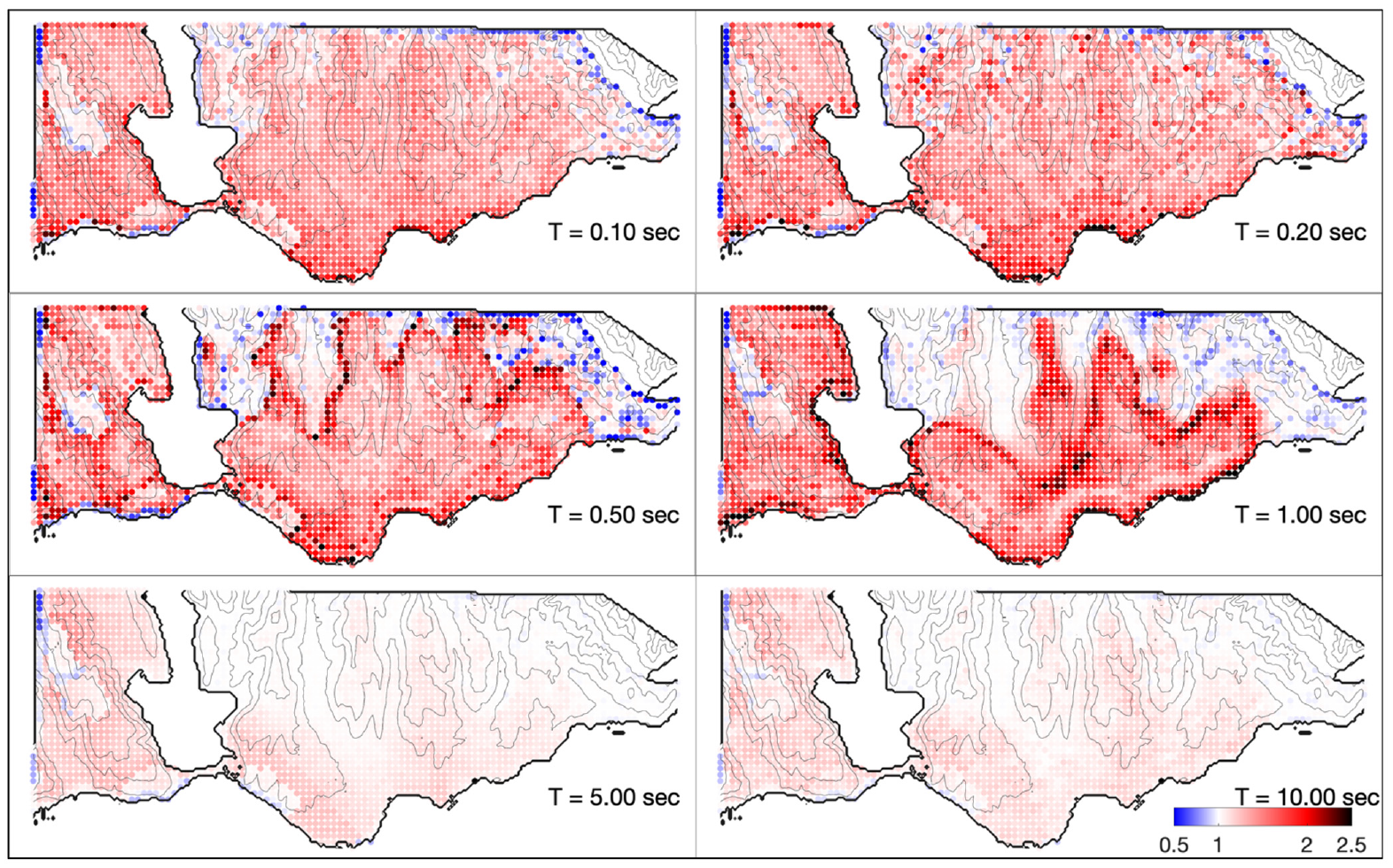
Horizontal S_a ratios of 3D GMS to 1D SRA.

Figure 9.

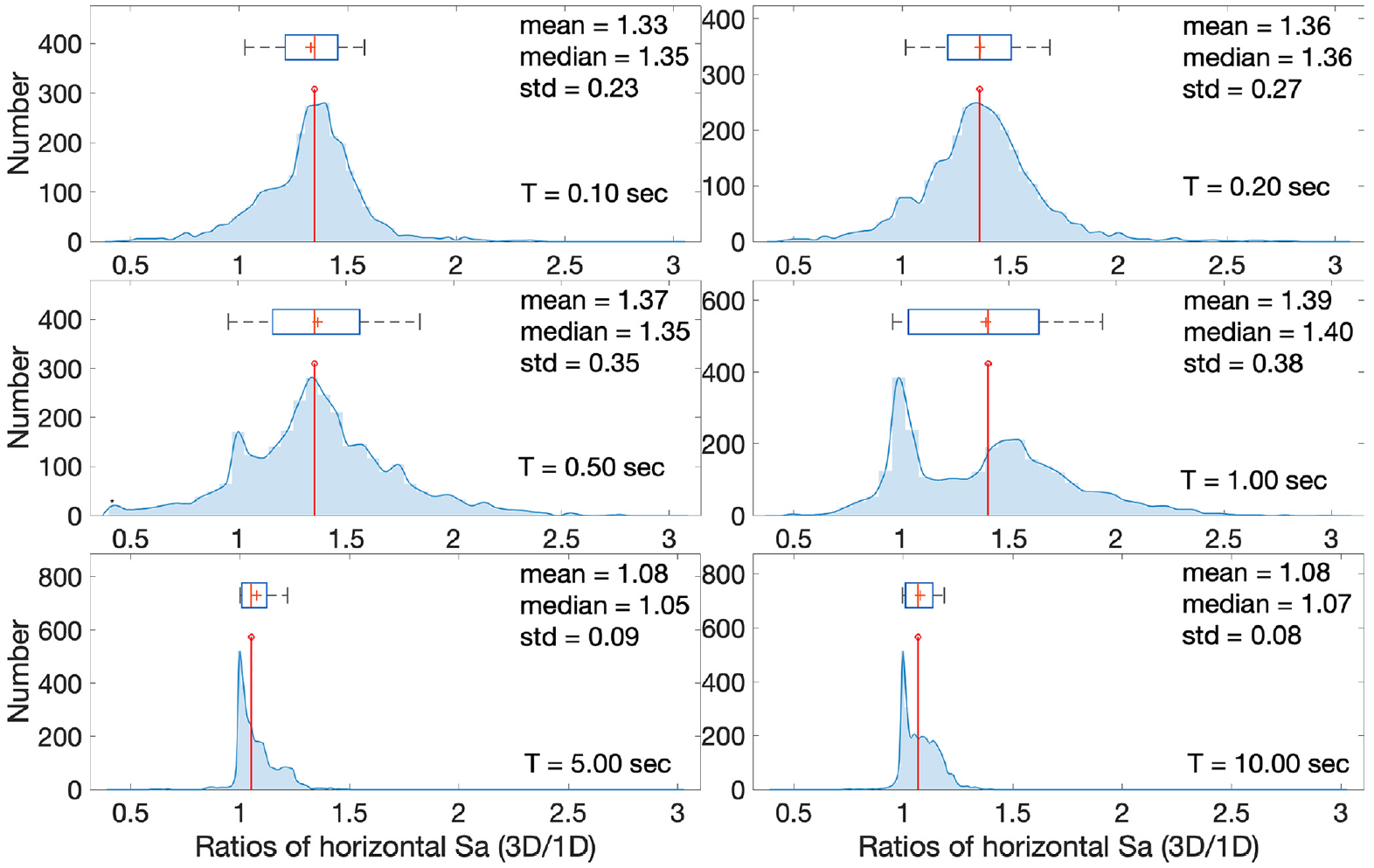
Distributions of S_a ratios of 3D GMS to 1D SRA. The vertical red line and cross symbol indicate the median and mean ratios, respectively.

Correlations of 3D/1D ratios and geotechnical and topographical parameters

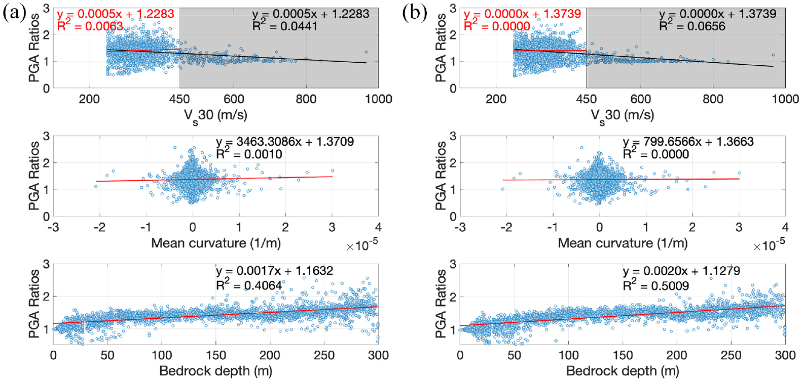
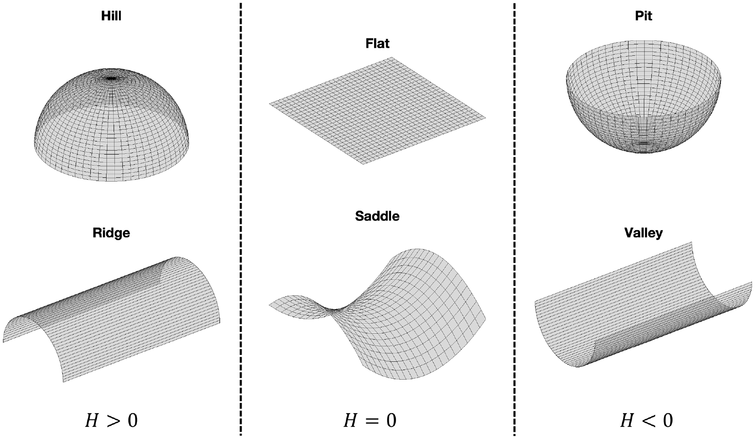
To further explore the root cause of the amplification/de-amplification factors due to 3D effects, we conduct linear regression analyses to examine possible correlations between 3D/1D ratios and three popular geotechnical and topographical parameters—that is, (1) $V_{s} 30$ ; (2) mean curvature of the ground surface considering topography; and (3) bedrock depth. By definition, the mean curvature (H) of a surface at a point is one-half the sum of the principal curvatures at that point (O’neill, 2006). Hence, a hill/ridge location has $H > 0$ , while a valley/pit area has $H < 0$ , and a flat/saddle surface has $H = 0$ (see Figure 10 for graphical representations). So, H can be used to depict the local topography of a site.

Figure 10.

Graphical representation of surfaces with different mean curvatures.

Figures 11 and 12 show scatter plots and fitted lines for PGA and PGV ratios, respectively. As seen, there is a large variability of PGA and PGV 3D/1D ratios, especially for those stations who have $V_{s} 30 < 450 m / s$ . We deduce this is due to three key factors:

The data points for 3D/1D ratios are collected from a total of 2912 stations and every station has a different bedrock depth, ranging from 0 to 300 m. For those stations who have $V_{s} 30 < 450 m / s$ normally have a softer soil layer and deeper bedrock depth than those with $V_{s} 30 \geq 450 m / s$ , and this can lead to a more distinct wave propagation pattern between 1D and 3D simulations.

Those stations that are adjacent to the coastline are likely to have very large (or small) 3D/1D ratios. This is because we do not have velocity data for the soil beneath the seabed, we simply make up a layered soil media for the water area. Such huge contrast and discontinuity in terms of soil velocity can result in a large variability of PGA and PGV 3D/1D ratios.

There are many important features in affecting ground motions that 1D simulations cannot capture, such as obliquely incident waves, surface topography, non-horizontal soil layers, complex reflections, refractions and diffractions, and so on.

Figure 11.

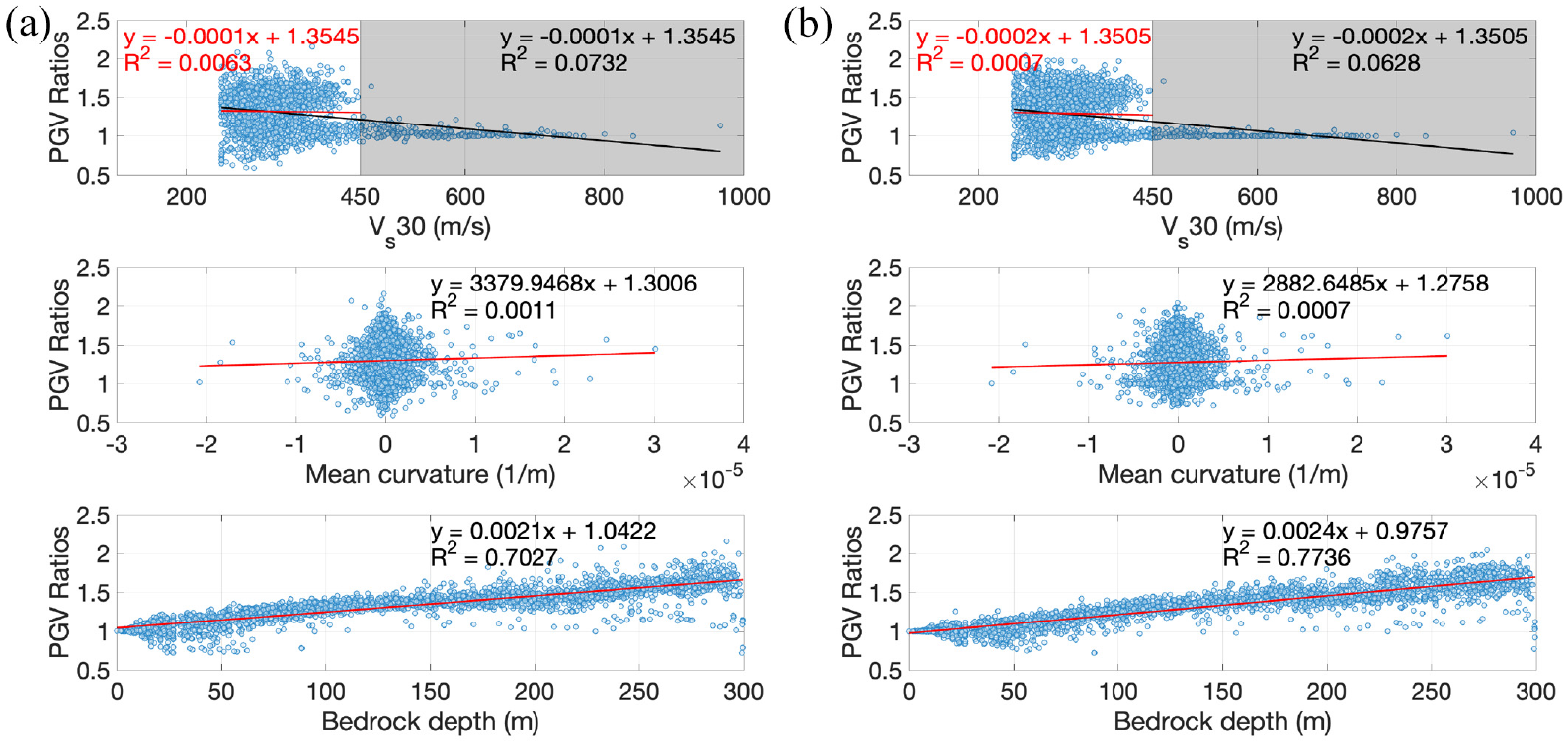
Linear regression analysis of the ratios (3D/1D) of horizontal (left) and vertical (right) PGAs and $V_{s} 30$ , mean curvature of the ground surface, and bedrock depth. The solid red and black lines in top-row plots represent the fitted line for the data with $V_{s} 30 < 450 m / s$ and entire data set, respectively: (a) horizontal and (b) vertical.

Figure 12.

Linear regression analysis of the ratios (3D/1D) of horizontal (left) and vertical (right) PGVs and $V_{s} 30$ , mean curvature of the ground surface, and bedrock depth. The solid red and black lines in top-row plots represent the fitted line for the data with $V_{s} 30 < 450 m / s$ and entire data set, respectively: (a) horizontal and (b) vertical.

Figure 13 displays regression analysis results between the bedrock depth and horizontal S_a ratios at six different periods. Please note that the y-value of each point represents the average 3D/1D ratio among 57 earthquakes for a given site. It is observed that bedrock depth has an evident linear relationship with all PGA, PGV, and S_a ratios in terms of $R^{2}$ values, which are rather negligible for $V_{s} 30$ and mean curvature. This is reasonable since bedrock depth significantly controls the depth of the soft soil layer and hence the site amplification behavior. $V_{s} 30$ only depends on the $V_{s}$ of the upper 30-m depth. However, many boreholes have bedrock depths of more than 30 m, even over 250 m. The mean curvature, H, at least in our study, is not a good index of topographic features affecting near-surface wave propagation. This is mainly because the surface topography in our domain of interest is relatively flat, with elevation only ranging from 0 to about 150 m. It is also interesting to see that the linear relationships between the bedrock depth and horizontal S_a ratios are varying at different periods. For medium periods, resonant behavior is detected—for example, at around 70 m for 0.5 s and 120 m for 1.0 s. A more linear trend is observed when the period increases.

Figure 13.

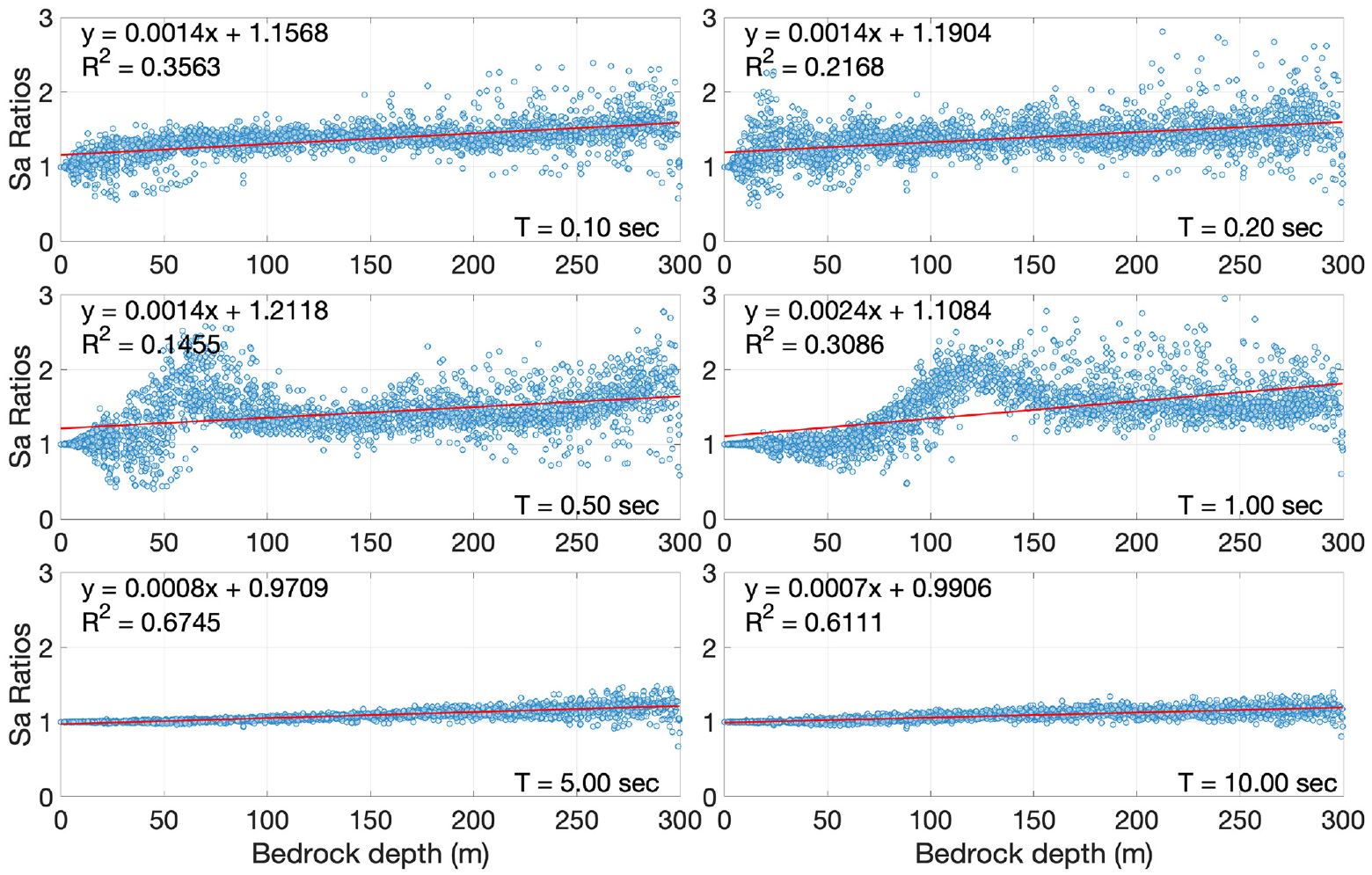
Linear regression analysis of the ratios (3D/1D) of horizontal S_as at different periods and bedrock depth.

Twelve representative stations

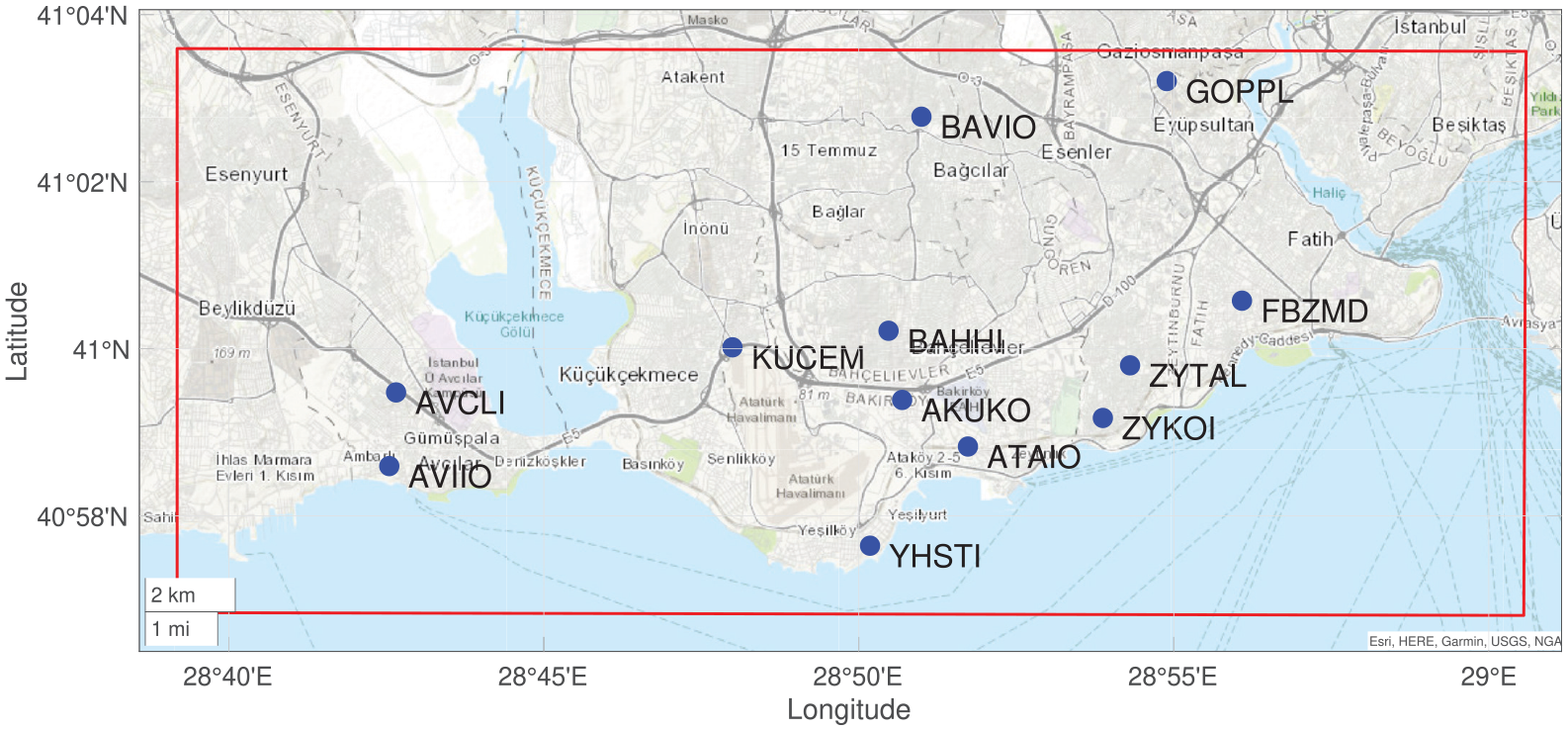
In this section, we consider 12 representative stations (see Figure 14 for their locations on the map), which have been used to validate our 3D GMS against recorded motions from the 2019 M_w 5.7 Silivri earthquake (Zhang et al., 2023), to further investigate the 3D effects on the 3D/1D ratios of PGA, PGV, and Sa, and their correlations with bedrock depth. Figure 15 shows the $V_{s}$ profiles of all 12 representative stations that were obtained from a previous microzonation study (LessLoss Integrated Project, 2004–2007). As seen, large variations of bedrock depth are observed among 12 stations, ranging from 14.8 m (BAVIO) to 296.0 m (YHSTI).

Figure 14.

Locations of 12 representative stations used in this study.

Figure 15.

$V_{s}$ profiles of 12 representative stations used in this study. The gray area depicts the engineering bedrock layer, which extends to a depth of 300 m.

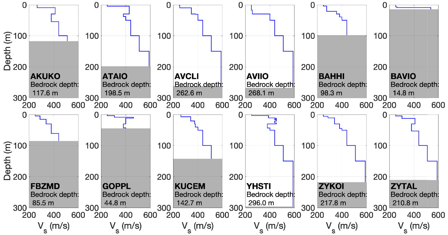
Figures 16 and 17 display box plots for the ratios of 3D to 1D PGAs and PGVs for these 12 representative stations, respectively. The box plot for each station is generated using the 3D/1D ratios from 57 earthquake simulations. It can be seen that the ratios of PGAs exhibit a similar behavior/trend to the ratios of PGVs, but they are slightly greater than the ratios of PGVs. Most stations (i.e. 11/12, except station GOPPL) show amplified responses. These stations, which have the greater amplification factors, such as stations AVIIO and YHSTI, also have large bedrock depths. On the contrary, stations BAVIO and GOPPL experience neutral or de-amplified behavior, and their bedrock depths are also the smallest ones among all 12 stations. This trend is consistent with what we discovered in the previous section.

Figure 16.

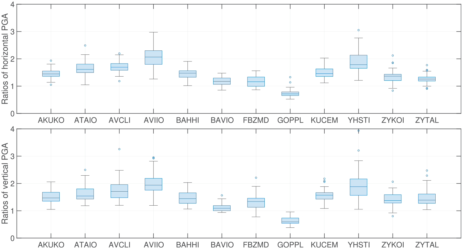
Box plots for the ratios of horizontal (top) and vertical (bottom) PGAs (3D/1D) of 12 representative stations used in this study.

Figure 17.

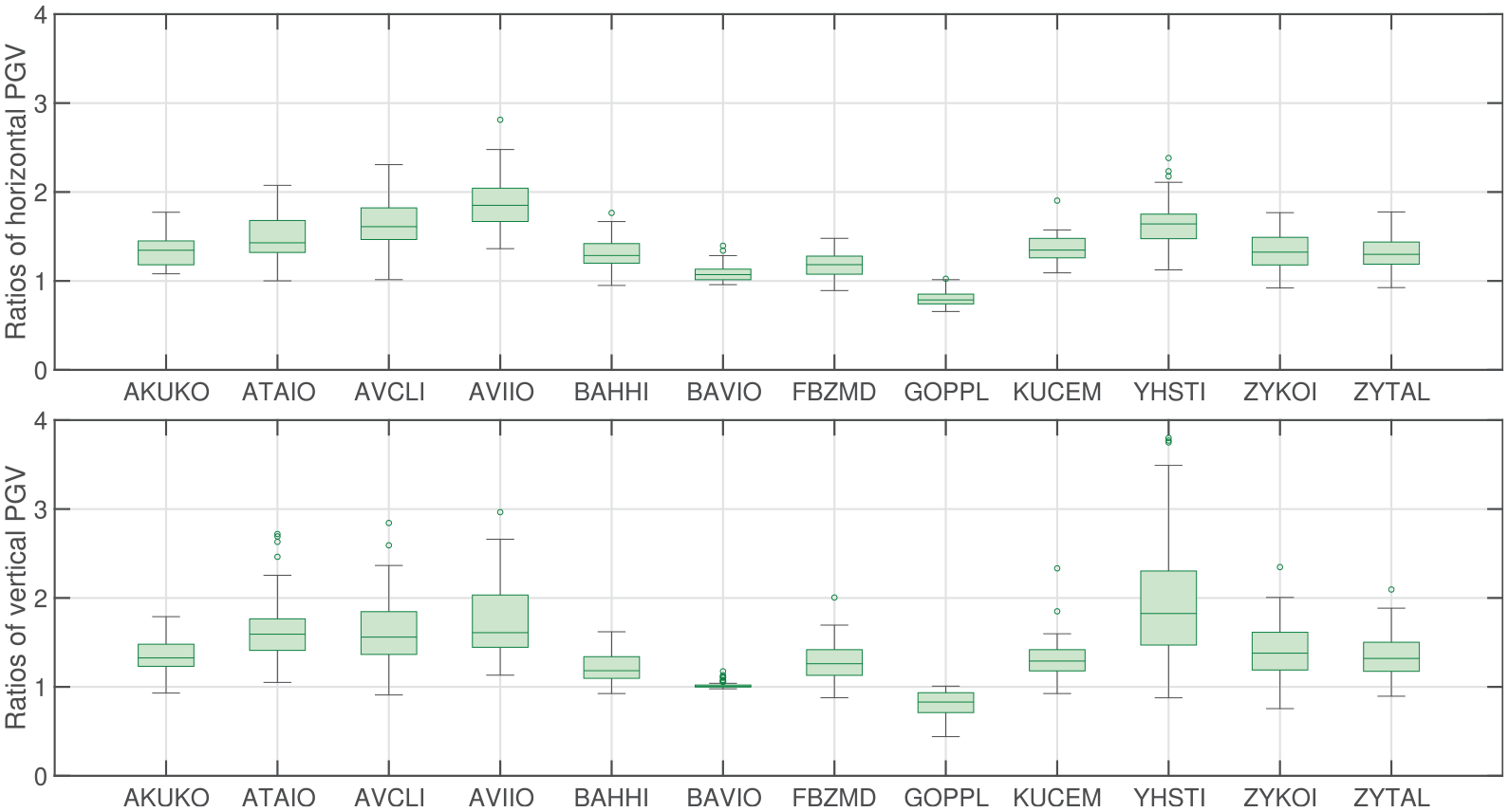
Box plots for the ratios of horizontal (top) and vertical (bottom) PGVs (3D/1D) of 12 representative stations used in this study.

In addition, it is worth discussing the performance of station GOPPL, which is the only station showing the de-amplified responses for both PGA and PGV ratios, and in both horizontal and vertical directions as well. From Figure 15, we see two noticeable $V_{s}$ reductions when the soil depth increases. And the $V_{s}$ of the last soil layer that is just above the bedrock is also very small compared to other stations, which leads to a big contrast of $V_{s}$ and hence soil stiffness. These factors eventually result in the de-amplified response observed for station GOPPL.

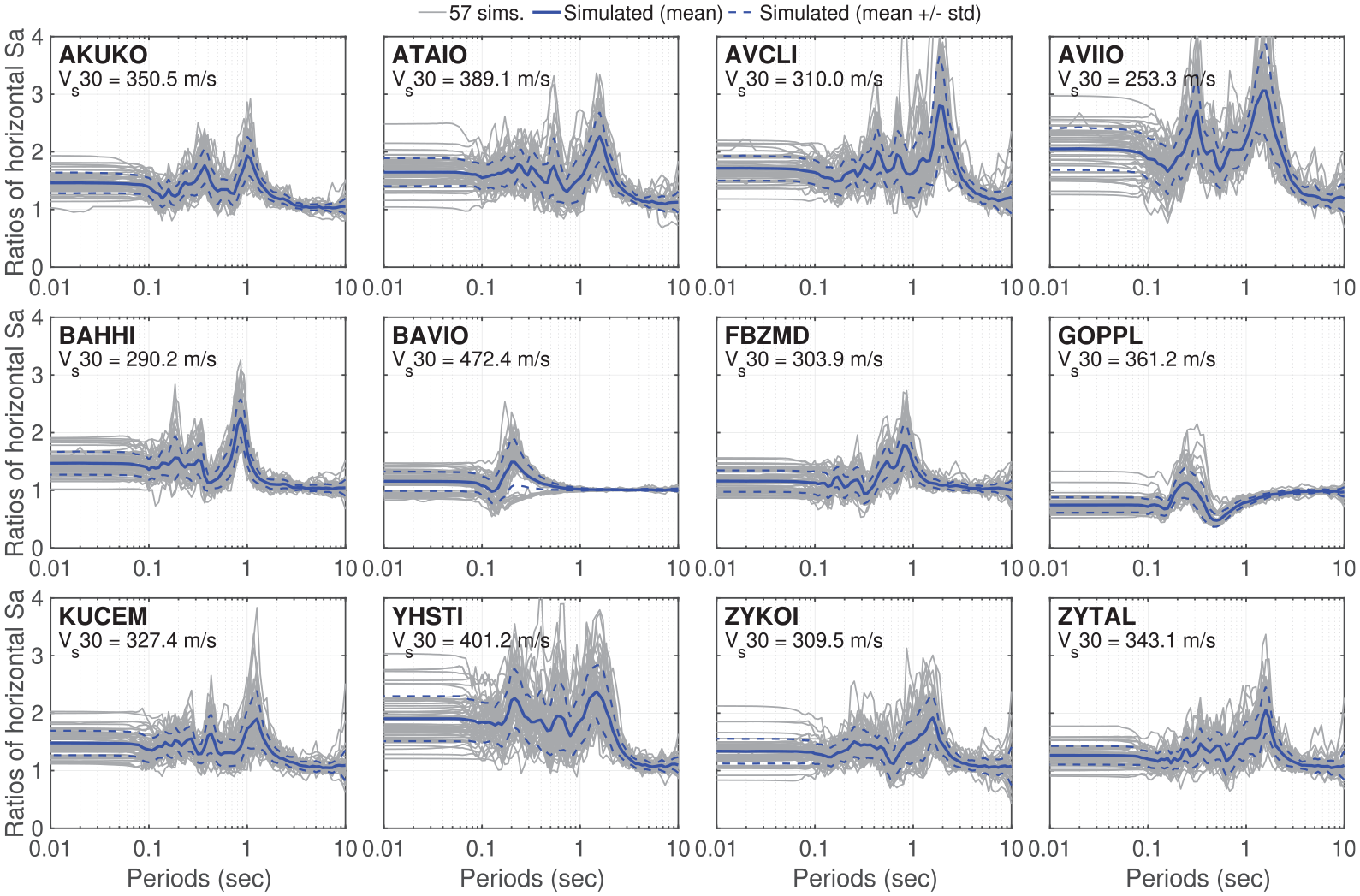
Figure 18 depicts 3D/1D ratios of the horizontal S_a curves from 0.01 to 10 s for the 12 representative stations. Each subplot has 57 gray curves, which correspond to 57 earthquake simulations. The solid blue curve represents the mean ratios among 57 simulations, and the two dashed blue curves are mean ± standard deviations. The ratios are close to 1 within the long-period range (e.g. $T > 5.0 s$ ) and exhibit fluctuations for periods between 0.1 and 3.0 s. In addition, these 12 stations exhibit different peak patterns—for example, two or more clear peaks (AKUKO, AVCLI, AVIIO, and YHSTI), one clear peak (ATAIO, BAHHI, BAVIO, GOPPL), and no clear peak (FBZMD, KUCEM, ZYKOI, and ZYTAL). The corresponding frequency at each peak represents the resonant frequency of ground motions that can amplify the 3D/1D ratios to the greatest possible extent for that site.

Figure 18.

Ratios of horizontal S_as (3D/1D) of 12 representative stations used in this study.

To quantify the site-specific feasibility of the 1D SRA, a taxonomy proposed by Tao and Rathje (2020) is utilized in this study. Specifically, the transfer functions (TFs) (Aki and Richards, 2002; Garcia-Suarez et al., 2022; Kramer, 1996) and the Horizontal-to-Vertical Spectral Ratios (HVSRs) (García-Jerez et al., 2016) are incorporated in the evaluation procedure. The empirical HVSR from the 3D GMS is computed to identify the first-mode resonant frequency of the site, and the within and outcrop TFs are used to distinguish true outcrop-resonances from pseudo-resonances (Tao and Rathje, 2020). The sites are then classified into four groups: dominated by only true-resonances (group A), both pseudo-resonances and true-resonances (group B), only pseudo-resonances (group C), and not modeled well using 1D SRA (group D). Figure 19 depicts the taxonomy workflow to categorize all four site groups. The site is considered as being well-characterized by 1D SRA if it falls into groups A, B, and C, whereas it is deemed unsuitable for 1D analysis if it belongs to Group D.

Figure 19.

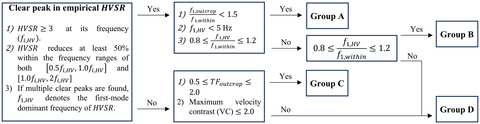
Taxonomy for assessing the feasibility of 1D SRA (Tao and Rathje, 2020).

In this study, all 12 representative stations are classified following the aforementioned criteria to assess their suitability of 1D SRA. As shown in Table 2, no clear peak is detected for all 12 stations, which is because their maximum HVSRs are no greater than 3. And 9 out of 12 stations are classified as Group D, which can explain the discrepancies between 1D SRA and 3D GMS. However, for those three sites that are classified as Group C, their 3D/1D ratios are not close to 1, either. This is mainly because the taxonomy approach proposed by Tao and Rathje (2020) is based on empirical HVSRs that are computed using real-life low-amplitude earthquake recordings. But our HVSRs are calculated from simulated ground motions, whose accuracy mainly depends on the quality of the 3D velocity model. Such discrepancies can make the taxonomy method limited in this study. The outcrop and within TFs and HVSR curves are shown in Figure 20.

Table 2.

Taxonomy results for 12 representative stations

Station ID	Clear peak	$f_{1, outcrop}$	$f_{1, within}$	$f_{1, HV}$	Maximum VC	Group
AKUKO	False	0.95	0.94	N/A	1.71	D
ATAIO	False	0.70	0.65	N/A	1.72	C
AVCLI	False	0.60	0.53	N/A	1.38	D
AVIIO	False	0.43	0.38	N/A	1.47	D
BAHHI	False	1.12	1.07	N/A	1.98	D
BAVIO	False	1.18	1.16	N/A	2.07	D
FBZMD	False	0.70	0.69	N/A	2.73	D
GOPPL	False	1.16	1.14	N/A	3.00	D
KUCEM	False	0.86	0.82	N/A	1.98	C
YHSTI	False	0.49	0.47	N/A	1.54	C
ZYKOI	False	0.62	0.61	N/A	2.03	D
ZYTAL	False	0.63	0.62	N/A	2.03	D

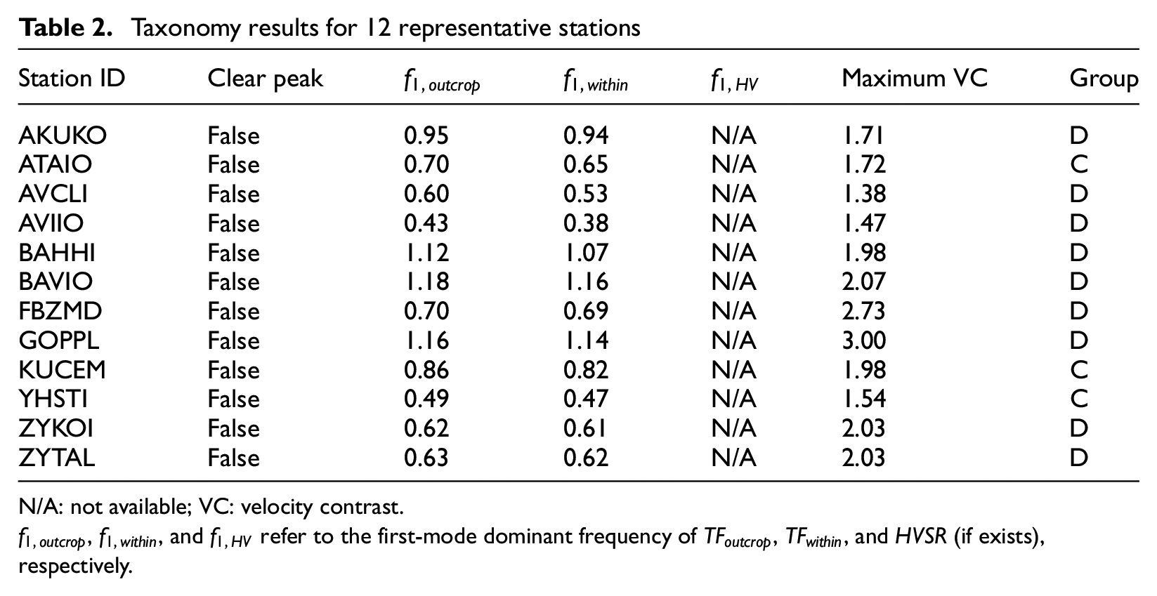
N/A: not available; VC: velocity contrast.

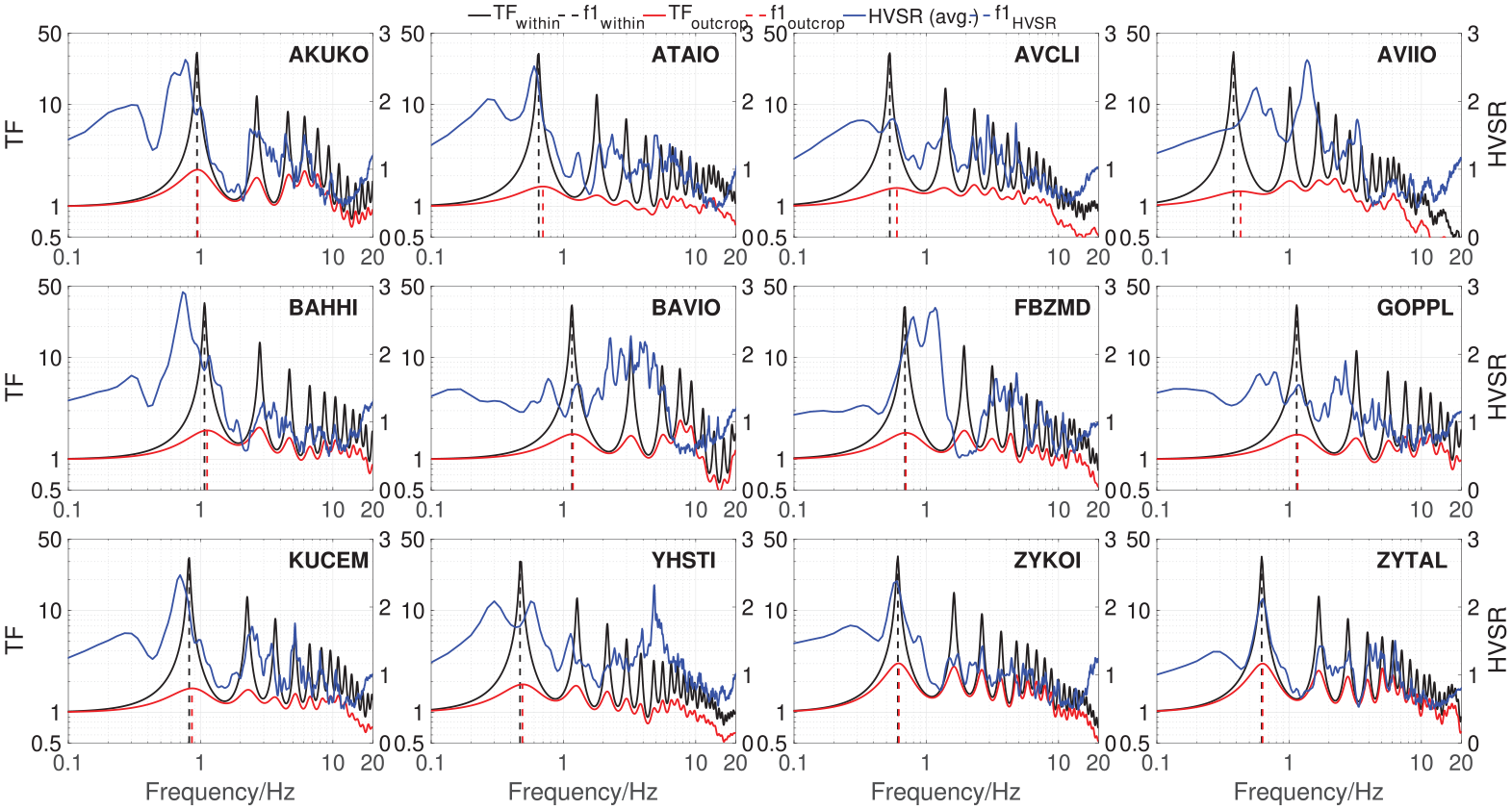
$f_{1, outcrop}$ , $f_{1, within}$ , and $f_{1, HV}$ refer to the first-mode dominant frequency of $T F_{outcrop}$ , $T F_{within}$ , and HVSR (if exists), respectively.

Figure 20.

Within and outcrop transfer functions and HVSRs of 12 representative stations used in this study. The HVSRs for each station are average HVSRs among 57 simulations.

Conclusion

By utilizing simulated ground motions from a suite of 57 3D physics–based broadband (from 0 to 8–12 Hz) GMSs for the Istanbul region, this study uses regional-scale 1D three-directional site response analyses for a total of 2912 borehole stations, which are distributed in an area of 30 km by 12.5 km with an approximately uniform distance of 250 m by 250 m between each other. Each borehole station is modeled as a 1D soil column with identical soil layers as used in 3D simulations. For each earthquake scenario, every 1D soil column is excited by the motions from 3D GMS that are recorded at the engineering bedrock level of the site where the soil column is located. Then, various IMs of ground surface motion—including both horizontal and vertical PGAs and PGVs, and spectral accelerations at multiple periods—are compared between the 1D SRA and 3D GMS.

For PGAs and PGVs, results show that roughly 90% of the site responses are amplified under 3D simulations, with median amplification factors of 1.4 and 1.3, respectively. As for horizontal S_a values, different behaviors are observed under different periods. The variations are reduced under long periods (i.e. $T > 5.0 s$ ), with 3D/1D ratios collapsed to 1.0–1.1. More dispersive responses are observed at periods from 0.1 to 1.0 s. Meanwhile, the median 3D/1D ratios increased to $1.35 ~ 1.40$ . The resulting 3D/1D ratios are mainly driven by two things that cannot be captured by the 1D approach: (1) Basin effects. In 3D simulations, the minimum element size ranges from 1.8 to 3.1 m (Zhang et al., 2023). However, the distance between two adjacent stations is about 250 m, which means that the 1D approach cannot accurately capture the variations of soil properties in between. Also, non-horizontal soil stratigraphy always occurs in 3D velocity models, but not in 1D. (2) Complex wave patterns. In 3D simulations, the dynamic fault rupture model produces realistic but complex wave patterns, which include inclined shear and compressional body waves, and laterally propagating surface waves. But the 1D SRAs are based on the assumption that the wave always vertically propagates along the soil column.

To further investigate the correlations between 3D/1D ratios and potential engineering parameters, we first select three commonly used parameters to represent: (1) soil conditions— $V_{s} 30$ ; (2) surface topography—H, median curvature; and (3) soil layer thickness—bedrock depth. Then, we perform the linear regression analysis. Results indicate that the 3D/1D ratios have a much stronger relationship with the bedrock depth compared with $V_{s} 30$ and the mean curvature. A linear trend is detected for all PGAs, PGVs, and long-period S_as. A deep bedrock depth stands for an overall thicker layer of soft soil, which can significantly magnify the ground responses under 3D wave propagation. Hence, the bedrock depth can be used for predicting the 3D/1D ratios for sites lacking instrumentation.

Finally, we adopt 12 stations, which have been used to validate our 3D GMS against the recorded earthquake in the past, as a case study. Similarly, most stations (11/12) have intensified responses, with median amplification factors ranging from 1.0 to 2.0. The only station which displays de-amplified performance has a relatively shallow bedrock depth, which is consistent with what we discern from the linear regression analysis.

This study comprehensively examined ground motion intensity predictions from 1D SRA in comparison to 3D GMS at a regional scale. It also explored the influence of various engineering parameters that are nominally considered to control 3D/1D amplification/de-amplification factors. However, please be advised that the accuracy of 3D physics–based simulation results heavily relies on the accuracy in fault rupture source modeling and quality of velocity model. Thus, further validations need to be performed in order to make the direct use of these 3D/1D ratios in real applications reliable. It is also worth noting that this study models the soil as a linear elastic material, which is unrealistic considering such large earthquake magnitudes and low shear wave velocities. In our future study, we will use advanced soil constitutive models to simulate the shallow crust and investigate the effects of soil nonlinearity on physics-based GMSs. Furthermore, the earthquake magnitude, fault depth, and distance can also play an important role on 3D/1D response. A comprehensive parametric study will be needed to explore their interlocked correlations.

Footnotes

Declaration of conflicting interests

The author(s) declared no potential conflicts of interest with respect to the research, authorship, and/or publication of this article.

Funding

The author(s) received no financial support for the research, authorship, and/or publication of this article.

ORCID iDs

Wenyang Zhang

Ertugrul Taciroglu

Notes

References

Abrahamson

(2006) Seismic hazard assessment: Problems with current practice and future developments. In:First European conference on earthquake engineering and seismology, 3–8 September, Geneva, pp. 3–8.

Aki

Richards

(2002) Quantitative Seismology. Herndon, VA: University Science Books.

Akinci

Aochi

Herrero

Pischiutta

Karanikas

(2017) Physics-based broadband ground-motion simulations for probable Mw ≥ 7.0 earthquakes in the Marmara sea region (Turkey) physics-based broadband ground-motion simulations for probable Mw ≥ 7.0 earthquakes. Bulletin of the Seismological Society of America 107: 1307–1323.

Bahrampouri

Rodriguez-Marek

(2023) One-dimensional site response analysis: Model error estimation. Bulletin of the Seismological Society of America 113: 401–416.

Baker

Bradley

Stafford

(2021) Seismic Hazard and Risk Analysis. Cambridge: Cambridge University Press.

Bradley

(2015.) Benefits of site-specific hazard analyses for seismic design in New Zealand. Bulletin of the New Zealand Society for Earthquake Engineering 48: 92–99.

de la Torre

Bradley

McGann

(2022.) 2D geotechnical site-response analysis including soil heterogeneity and wave scattering. Earthquake Spectra 38: 1124–1147.

Douglas

Aochi

(2016.) Assessing components of ground-motion variability from simulations for the Marmara Sea region (Turkey). Bulletin of the Seismological Society of America 106: 300–306.

Chen

Yin

Zhang

Xue

Liu

Yin

Yang

Chen

(2017) 18.9-Pflops nonlinear earthquake simulation on Sunway TaihuLight: Enabling depiction of 18-Hz and 8-meter scenarios. In: Proceedings of the international conference for high performance computing, networking, storage and analysis, Denver, CO, 12–17 November. New York: IEEE.

10.

García-Jerez

Piña-Flores

Sánchez-Sesma

Luzón

Perton

(2016) A computer code for forward calculation and inversion of the H/V spectral ratio under the diffuse field assumption. Computers and Geosciences 97: 67–78.

11.

Garcia-Suarez

González-Carbajal

Asimaki

(2022) Analytical 1D transfer functions for layered soils. Soil Dynamics and Earthquake Engineering 163: 107532.

12.

Graves

(1998) Three-dimensional finite-difference modeling of the San Andreas fault: Source parameterization and ground-motion levels. Bulletin of the Seismological Society of America 88: 881–897.

13.

Huang

Mccallen

(2023) Predicament of the 1D assumption in site response analysis and implications for vertical ground motion assessment. In: 9th International Conference on Computational Methods in Structural Dynamics and Earthquake Engineering, Athens, 12–14 June 2023.

14.

Ichimura

Fujita

Quinay

PEB

Maddegedara

Hori

Tanaka

Shizawa

Kobayashi

Minami

(2015) Implicit nonlinear wave simulation with 1.08T DOF and 0.270T unstructured finite elements to enhance comprehensive earthquake simulation. In: SC’15: Proceedings of the international conference for high performance computing, networking, storage and analysis, Austin, TX, 15–20 November 2015, pp. 1–12. New York: IEEE.

15.

Idriss

Boulanger

(2008) Soil Liquefaction during Earthquakes. Oakland, CA: Earthquake Engineering Research Institute.

16.

Infantino

Mazzieri

Özcebe

Paolucci

Stupazzini

(2020) 3D physics-based numerical simulations of ground motion in Istanbul from earthquakes along the Marmara segment of the north Anatolian fault. Bulletin of the Seismological Society of America 110: 2559–2576.

17.

Kramer

(1996) Geotechnical Earthquake Engineering. New Delhi, India: Pearson Education.

18.

Lee

S-J

Chen

H-W

Liu

Komatitsch

Huang

B-S

Tromp

(2008) Three-dimensional simulations of seismic-wave propagation in the Taipei basin with realistic topography based upon the spectral-element method. Bulletin of the Seismological Society of America 98: 253–264.

19.

LessLoss Integrated Project (2004–2007) Risk Mitigation for Earthquakes and Landslides Integrated Project. Tech. Rep. Sixth Framework Programme, Priority 1.1.6.3 global change and ecosystems. Project No. GOCE-CT-2003-505488.

20.

McCallen

Petersson

Rodgers

Pitarka

Miah

Petrone

Sjogreen

Abrahamson

Tang

(2021) EQSIM—A multidisciplinary framework for fault-to-structure earthquake simulations on exascale computers part I: Computational models and workflow. Earthquake Spectra 37: 707–735.

21.

McGann

Bradley

Wotherspoon

Lee

(2021) Basin effects and limitations of 1D site response analysis from 2D numerical models of the Thorndon basin. Bulletin of the New Zealand Society for Earthquake Engineering 54: 21–30.

22.

Madiai

Facciorusso

Gargini

Baglione

(2016) 1D versus 2D site effects from numerical analyses on a cross section at Barberino di Mugello (Tuscany, Italy). Procedia Engineering 158: 499–504.

23.

Makra

Chávez-García

(2016) Site effects in 3D basins using 1D and 2D models: An evaluation of the differences based on simulations of the seismic response of Euroseistest. Bulletin of Earthquake Engineering 14: 1177–1194.

24.

Mazzoni

McKenna

Scott

Fenves

(2006) OpenSees command language manual. Pacific Earthquake Engineering Research (PEER) Center 264: 137–158.

25.

NHERP (2015) Recommended seismic provisions for new buildings and other structures. Technical Report, FEMA P-1050. Washington, DC: Building Seismic Safety Council. Available at: https://www.fema.gov/sites/default/files/2020-07/fema_nehrp-seismic-provisions-new-buildings_p-1050-1_2015.pdf

26.

Olsen

Nigbor

Konno

(2000) 3D viscoelastic wave propagation in the Upper Borrego Valley, California, constrained by borehole and surface data. Bulletin of the Seismological Society of America 90: 134–150.

27.

O’neill

(2006) Elementary Differential Geometry. New York: Elsevier.

28.

Oral

Ayoubi

Ampuero

Asimaki

Bonilla

(2022) Kathmandu Basin as a local modulator of seismic waves: 2-D modelling of non-linear site response under obliquely incident waves. Geophysical Journal International 231: 1996–2008.

29.

OYO (2007) Production of microzonation report and maps—on European Side (south). Technical Report. Final Report to Istanbul Metropolitan Municipality. Available at: https://cordis.europa.eu/project/id/209871/reporting/es

30.

Özcebe

Smerzini

Paolucci

Pourshayegan

Plata

Lai

Zuccolo

Bozzoni

Villani

(2019) On the comparison of 3D, 2D, and 1D numerical approaches to predict seismic site amplification: The case of Norcia basin during the M6. 5 2016 October 30 earthquake. In: Earthquake geotechnical engineering for protection and development of environment and constructions, Roma, 17–20 June, pp. 4251–4258. Boca Raton, FL: CRC Press.

31.

Pitarka

Akinci

De Gori

Buttinelli

(2022) Deterministic 3D ground-motion simulations (0–5 Hz) and surface topography effects of the 30 October 2016 Mw 6.5 Norcia, Italy, earthquake. Bulletin of the Seismological Society of America 112: 262–286.

32.

Pitarka

Irikura

Iwata

Sekiguchi

(1998) Three-dimensional simulation of the near-fault ground motion for the 1995 Hyogo-ken Nanbu (Kobe), Japan, earthquake. Bulletin of the Seismological Society of America 88: 428–440.

33.

Poursartip

Fathi

Tassoulas

(2020) Large-scale simulation of seismic wave motion: A review. Soil Dynamics and Earthquake Engineering 129: 105909.

34.

Pretell

Ziotopoulou

Abrahamson

(2022) Numerical investigation of VS spatial variability effects on the seismic response estimated using 2D and 1D site response analyses. In: Geo-congress, pp. 205–215. Available at: https://ascelibrary.org/doi/10.1061/9780784484043.020

35.

Rathje

Kottke

Trent

(2010) Influence of input motion and site property variabilities on seismic site response analysis. Journal of Geotechnical and Geoenvironmental Engineering 136: 607–619.

36.

Riaño

Reyes

Yamn

Bielak

Taborda

Restrepo

(2021) Integration of 3D large-scale earthquake simulations into the assessment of the seismic risk of Bogota, Colombia. Earthquake Engineering & Structural Dynamics 50: 155–176.

37.

Roten

Cui

Olsen

Day

Withers

Savran

Wang

(2016) High-frequency nonlinear earthquake simulations on petascale heterogeneous supercomputers. In: SC’16: Proceedings of the international conference for high performance computing, networking, storage and analysis, Salt Lake City, UT, 13–18 November, pp. 957–968. New York: IEEE.

38.

Seylabi

Restrepo

Taborda

Asimaki

(2021) Deterministic ground motion simulations with shallow crust nonlinearity at Garner Valley in Southern California. Earthquake Engineering & Structural Dynamics 50: 43–59.

39.

Smerzini

Paolucci

Stupazzini

(2011) Comparison of 3D, 2D and 1D numerical approaches to predict long period earthquake ground motion in the Gubbio plain, Central Italy. Bulletin of Earthquake Engineering 9: 2007–2029.

40.

Stanzione

West

Evans

Minyard

Ghattas

Panda

(2020) Frontera: The evolution of leadership computing at the national science foundation. In: Practice and Experience in Advanced Research Computing, 23–27 July, pp. 106–111. New York: ACM.

41.

Stewart

Chiou

S-J

Bray

Graves

Somerville

Abrahamson

(2002) Ground motion evaluation procedures for performance-based design. Soil Dynamics and Earthquake Engineering 22: 765–772.

42.

Stewart

Fenves

Seed

(1999) Seismic soil-structure interaction in buildings. I: Analytical methods. Journal of Geotechnical and Geoenvironmental Engineering 125: 26–37.

43.

Stupazzini

Paolucci

Igel

(2009) Near-fault earthquake ground-motion simulation in the Grenoble valley by a high-performance spectral element code. Bulletin of the Seismological Society of America 99: 286–301.

44.

Tao

Rathje

(2020) Taxonomy for evaluating the site-specific applicability of one-dimensional ground response analysis. Soil Dynamics and Earthquake Engineering 128: 105865.

45.

Ramirez-Guzman

Bielak

Ghattas

K-L

O’hallaron

(2006) From mesh generation to scientific visualization: An end-to-end approach to parallel supercomputing. In: SC’06: Proceedings of the 2006 ACM/IEEE conference on supercomputing, Tampa, FL, 11–17 November. New York: IEEE.

46.

Zhang

Crempien

Kurtulus

Chen

P-Y

Arduino

Taciroglu

(2023) A suite of broadband physics-based ground motion simulations for the Istanbul region. Earthquake Engineering & Structural Dynamics 52: 1161–1181.

47.

Zhang

Liu

Shokrabadi

Dehghanpoor

Taciroglu

(2022) Nonlinear seismic fragility assessment of tall buildings equipped with tuned mass damper (TMD) and considering soil-structure interaction effects. Bulletin of Earthquake Engineering 20: 3469–3483.

48.

Zhang

Restrepo

Crempien

Erkmen

Taborda

Kurtulus

Taciroglu

(2021) A computational workflow for rupture-to-structural-response simulation and its application to Istanbul. Earthquake Engineering & Structural Dynamics 50: 177–196.

49.

Zhang

Shokrabadi

Bozorgnia

Taciroglu

(2020) A methodology for fragility analysis of buried water pipes considering coupled horizontal and vertical ground motions. Computers and Geotechnics 126: 103709.

A comparison of ground motions predicted through one-dimensional site response analyses and three-dimensional wave propagation simulations at regional scales

Abstract

Keywords

Introduction

Problem background

1D SRA

1D SRA versus 3D GMS

PGA

PGV

Spectral acceleration (SA)

Correlations of 3D/1D ratios and geotechnical and topographical parameters

Twelve representative stations

Conclusion

Footnotes

Declaration of conflicting interests

Funding

ORCID iDs

Notes

References

Spectral acceleration (S_A)