Sage Journals: Discover world-class research

Abstract

Earthquake records collected at dense arrays of strong-motion stations are often utilized in microzonation studies to evaluate the changes in site response due to variability in site conditions across a region. These studies typically begin with calculating Fourier spectral amplification(s) and then transition to performing engineering site response analyses. It has proven difficult to utilize Fourier spectral amplification(s) to define the appropriate elastic response spectr(um)/(a) for a site or sites. This is because, first, the ground motions recorded at these strong-motion stations have lower intensity and hence do not show the nonlinear site effects observed during higher-intensity earthquakes and, second, Fourier and response spectral amplitudes measure different aspects of ground motions. The strong-motion stations in Anchorage, Alaska, have been recording earthquakes in the region for the last three decades. This study utilizes a database of 95 events from 2004 to 2019 to calculate Fourier spectral amplifications at 35 stations using the generalized inversion technique (GIT). Estimated response spectra have been evaluated at each site by applying those Fourier spectral amplifications to a response spectrum of a reference station through random vibration theory (RVT). Correction factors are also applied within the approach to account for nonlinear site effects. This RVT-based approach is tested using ground motions recorded during the M_W 7.1 2018 Anchorage Earthquake, and close matches between measured and predicted response spectra are found. The method is then compared with site response analyses using a calibrated 1D equivalent linear (EQL) model of the Delaney Park Downhole Array site. Estimated spectra using the RVT-based approach are, finally, compared with those using Next Generation Attenuation Subduction (NGA-Sub) and NGA-West2 ground-motion models. The proposed method provides a coherent and straightforward way to use GIT-derived Fourier spectral amplifications to directly estimate site-specific response spectra, accounting for nonlinear site effects and without requiring engineering characterization of subsurface soil conditions.

Keywords

Earthquake site response analysis random vibration theory spectral amplification microzonation

Introduction

The city of Anchorage, located in southcentral Alaska, is Alaska’s most populous city, with approximately half of the state’s population. Southcentral Alaska is situated in a very active tectonic region near the edges of the North American and the subducting Pacific plates. This region was significantly impacted by the 1964 Moment Magnitude (M_W) 9.2 Great Alaska Earthquake (Hansen, 1965), the second-largest earthquake on record (USGS.gov, 2020). Since the 1970s, strong-motion sensors have been installed in Anchorage for a better understanding of ground-motion variability across the city. Several studies have performed site response analyses in the frequency domain through methods such as standard spectral ratio (SSR) and horizontal to vertical spectral ratio (HVSR) (see, e.g. Borcherdt, 1970 and Ghofrani and Atkinson, 2014, for a discussion of these techniques) using the recorded ground motions at strong-motion stations. However, many of these stations have not been appropriately characterized through subsurface soil studies. Fourier amplitude spectra (FAS) of the recorded ground motions are used to compute SSR and HVSR. Although newer ground motion models and other tools are utilizing FAS more often (e.g. Bayless and Abrahamson, 2019), engineers often prefer response spectra, rather than FAS, because they better predict building and other structural responses. It should be noted that FAS more closely represent free-field ground motions compared with response spectra because response spectra are filtered through single-degree-of-freedom oscillators. This article aims to provide a methodology to utilize the results from spectral amplification studies, even from those primarily based on data from low-magnitude earthquakes, to estimate site response spectra that account for nonlinear soil behavior and without requiring detailed soil characterization. This will allow the engineering community to utilize, more efficiently, years of measured ground motions to understand engineering site response, especially at sites with poorly characterized soil conditions.

The following sections begin by presenting the tectonic setting and geologic conditions in Anchorage, followed by a description of the strong-motion data set used in this study. A brief description of the time history processing and Fourier spectral amplification analysis of the data set is provided. Then the methodology to calculate site response spectra utilizing Fourier spectral amplification results, combined with random vibration theory (RVT), is described. Several examples of its use are then presented and evaluated, with a final discussion on other potential applications.

Tectonic setting and seismicity

Alaska is situated in one of the most tectonically active regions globally with, for example, the Alaska Earthquake Center (AEC) recording more than 54,000 earthquakes across the state in 2018 (AEC, 2021), including the M_W 7.1 Anchorage Earthquake (Figure 1). Anchorage sits at the edge of the North American plate, where the Pacific plate converges at a rate of 55 mm/year (Haeussler, 2008). This region, known as the Alaska-Aleutian megathrust, experiences, on average, an M_W 7 or greater earthquake every 11 years (West et al., 2020).

Figure 1.

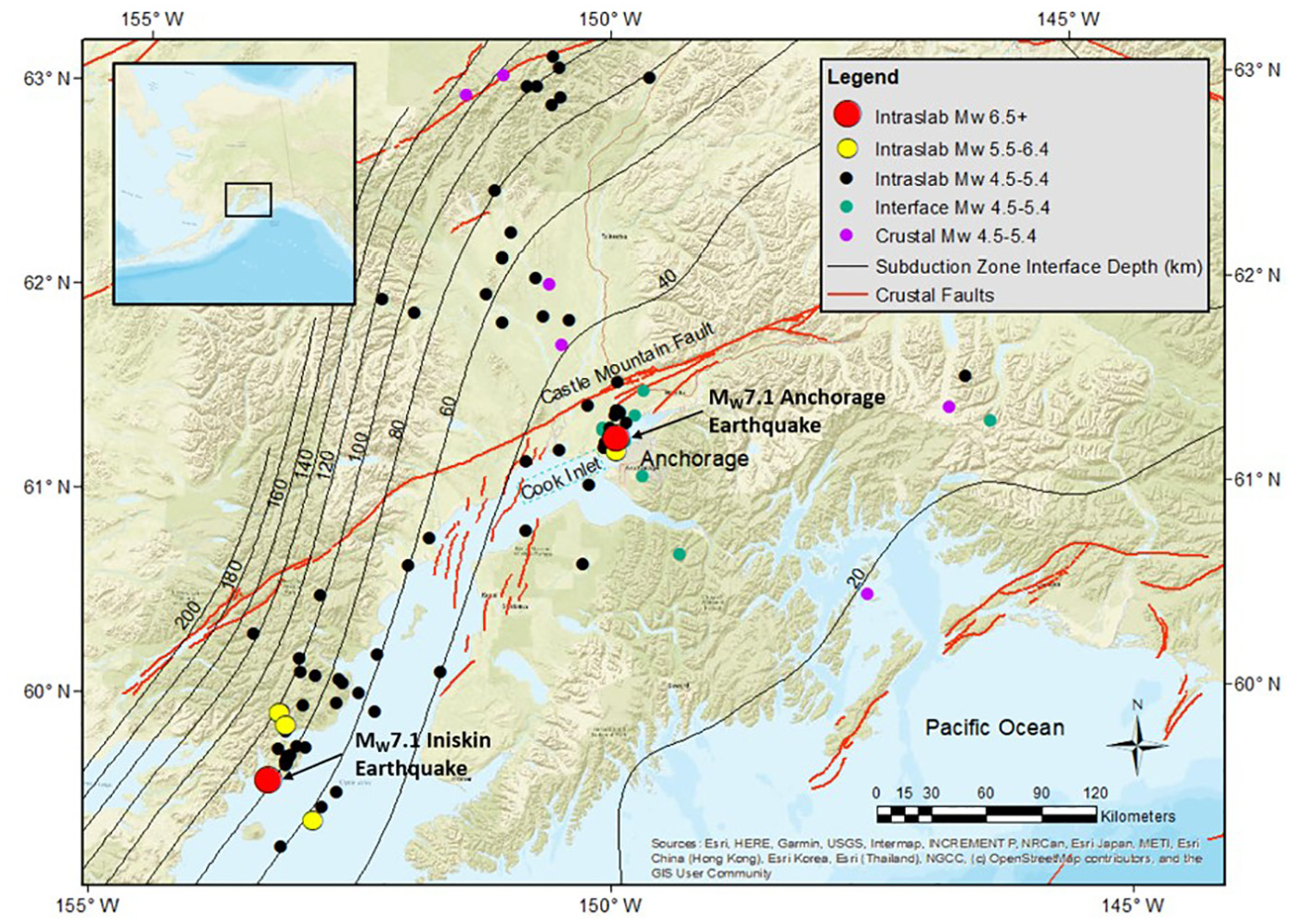
The tectonic setting of Southcentral Alaska, including contours of the interface between the North American and the subducting Pacific plates (using Slab 2.0; Hayes, 2018) and crustal faults as identified by Koehler (2013). The colored circles indicate the epicenters of the earthquakes used in this study, which have been divided into intraslab, interface, and crustal events.

Several sources, including the interface, intraslab, and crustal sources, are responsible for these earthquakes (Wesson et al., 2007). The intraslab events within the subducting Pacific plate are the most common. As an example, the 2018 M_W 7.1 Anchorage Earthquake was an intraslab event. In addition, several crustal sources can impact Anchorage, including the Castle Mountain Fault north of Anchorage, which is estimated to be capable of an M_W 7 to 7.5 earthquake (Koehler, 2013; Wesson et al., 2007).

Geology

The geologic setting below Anchorage is as intricate as the tectonic setting, as it has been greatly affected by the advances and retreats of various glaciers in the region, resulting in complex soil stratigraphy. The simplified surficial geology is presented in Figure 2. The Chugach Mountains, composed of lightly metamorphosed greywacke, rise at the city’s eastern border (Wilson et al., 2012). Dense glacial till overlies the greywacke and is found at the surface in the lower reaches of the Chugach Mountains to the east, but it is encountered at depth to the west (Combellick, 1999; Updike and Ulery, 1986). Glacial outwash and alluvial deposits are found in the northern portion of Anchorage, often overlying glacial till.

Figure 2.

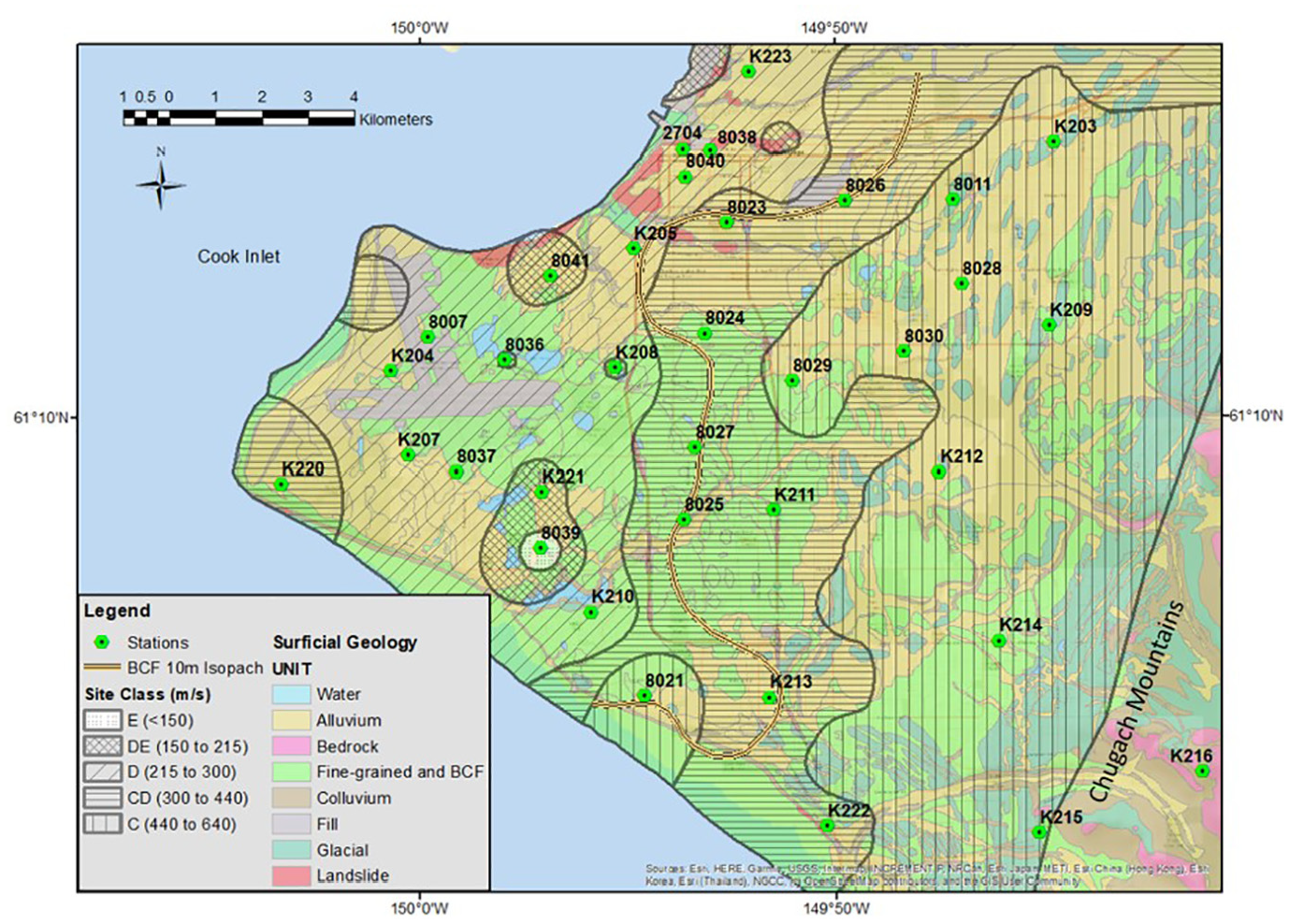
A simplified geologic map of Anchorage with strong-motion station locations. Hatching identifies the site class based on estimated V_S30 (Thornley et al., 2021c). A 10 m isopach line is added from Combellick (1999) to show the geologic break in Bootlegger Cove Formation (BCF) thickness, where the BCF becomes thinner to the east of the line.

The Bootlegger Cove Formation (BCF), due to glaciolacustrine deposition, consists of various facies of sand, silt, and clay (Updike and Ulery, 1986). The BCF is found in the city’s central and western portions. The more sensitive clay layers of the BCF have been identified as the weak soil that caused significant deformations and slope failures in the 1964 Great Alaska Earthquake. The BCF ranges in thickness up to 60 m, with its deepest portions found in the city’s western-central part (Ulery and Updike, 1983). The BCF grades to deltaic deposits of silt and fine sand on the western edge of Anchorage. The shear-wave velocities of the BCF are dependent on the facies, with the facies (generally located in the central-western portion of the city) having shear-wave velocities less than 180 m/s to the stiffer facies having shear-wave velocities greater than 360 m/s. The variability of these subsurface soil conditions affects the site response across Anchorage (Thornley et al., 2021b).

Strong-motion stations and data set

The current Anchorage network consists entirely of modern digital accelerometers (mostly Kinemetrics Basalt sensors) with sampling rates of 200 Hz. The 35 strong-motion stations used for this study are distributed across various surficial geologic conditions, as shown in Figure 2. Station K216, located within the Chugach Mountains (Figure 2), is located on a rock outcrop and is commonly used as a rock reference station. The other stations used in this study are located at soil sites. Additional details for the strong-motion stations are provided in Table 1 in the electronic supplement. These stations are operated and maintained with collaboration between the AEC and the United States Geological Survey (USGS). In addition to surface strong-motion stations, the Delaney Park Downhole Array (DPDA), operated by the University of California Santa Barbara and identified as Station 8040, was installed in 2004 (Figure 2). This comprises a surface sensor and six subsurface accelerometers sensors at varying depths of up to 60 m below the ground surface. Between 2005 and early 2019, approximately 95 earthquakes within 300 km, ranging from M_W 4.5 to M_W 7.1, were recorded at the strong-motion stations across Anchorage. The acceleration time histories were processed prior to performing data analysis. A detailed account of the full processing of the data is described in Thornley et al. (2021b). In all, 1,727 three-component records from the 95 events were retained after processing for this analysis.

Table 1.

Ground motions utilized for the DPDA calibrated model comparison with the RVT-based technique

Event^a	Station^a	Magnitude^a	V_S30(m/s)^a	Maximum ShearStrain (%)^b	Shear StrainIndex (%)^b	SurfacePGA (g)^b
Duzce, Turkey	Lamont 1060	7.14	782	0.020	0.022	0.06
Chi-Chi, Taiwan	TTN025	7.62	705	0.019	0.016	0.06
Hector Mine	Hector	7.13	726	0.202	0.170	0.33
Kocaeli, Turkey	Gebze	7.51	792	0.091	0.124	0.17

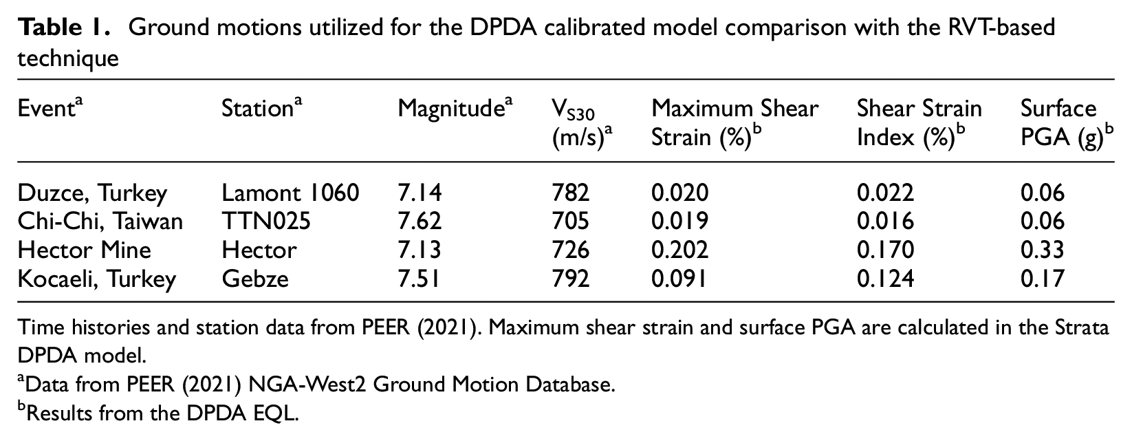
Time histories and station data from PEER (2021). Maximum shear strain and surface PGA are calculated in the Strata DPDA model.

Data from PEER (2021) NGA-West2 Ground Motion Database.

Results from the DPDA EQL.

Site spectral amplification evaluation

Once processed, the data set for the 35 strong-motion stations and 95 events was used to evaluate the site response variability across Anchorage. The generalized inversion technique (GIT), which was first developed by Andrews (1986), was utilized to perform the analysis. GIT is an efficient method for estimating the spectral amplification of many sites compared with a selected reference site (e.g. Bindi et al., 2017; Dutta et al., 2003; Laurenzano et al., 2019; Oth et al., 2009; Parolai et al., 2000). One of the benefits of GIT is its ability to use a large number of earthquakes at a large number of stations and obtain spectral amplification results at each station, even when not all stations recorded all earthquakes. The GITANES (Version 1.3) package, implemented in MATLAB by Klin (2019), was used for this analysis.

While three-component time histories are used as inputs to GITANES, only the horizontal orthogonal components (E-W for the east-west component and N-S for the north-south component) are used to calculate the response spectral amplification functions (SAFs). The two orthogonal SAFs were combined using the following equation to calculate an equivalent average spectral amplification function (EAF) over the selected range of frequencies (f) for each station evaluated:

EAF (f) = \sqrt{\frac{1}{2} [SA F_{E - W} {(f)}^{2} + SA F_{N - S} {(f)}^{2}]} .

(1)

The EAF for each station represents the spectral amplification compared with the selected reference station (Station K216 in this study). The range of frequencies utilized in this study ranged from 0.25 to 10 Hz or 0.1 to 4 s, which roughly covers the natural periods of buildings between 1 and 40 stories, encompassing the range of building types in Anchorage.

Once the spectral amplifications are calculated for each of the strong-motion stations, they can be used to understand the variability of site response across Anchorage, which is related to the changes in geologic conditions, especially from east to west (Thornley et al., 2021b). For example, the EAF for a site in eastern Anchorage (K212), with a shallow soil layer over dense glacial till (Combellick, 1999), is presented in Figure 3a, and the EAF for a station in western Anchorage, with a BCF thickness of more than 20 m and more than 40 m to dense glacial till (Updike and Ulery, 1986), is presented in Figure 3b. In general, the stations in the eastern portion of the city have higher spectral amplifications at higher frequencies, indicating stiff sites (higher shear-wave velocities), while the western portion has much higher spectral amplifications at lower frequencies, signifying softer sites (thick soil sites with lower shear-wave velocities).

Figure 3.

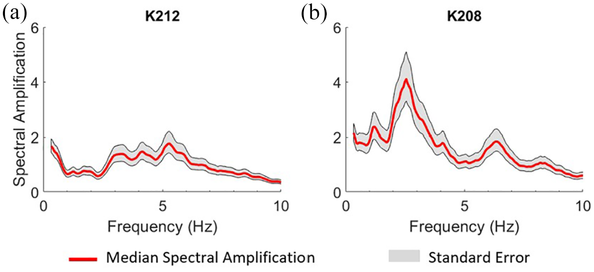
Fourier spectral amplification (ratio of the selected site and the reference site) for a station located on a shallow soil deposit over dense glacial till (a) and a station with more than 40 m of variable soil, including soft silts and clays, over dense glacial till (b). The gray shading indicates the calculated standard error.

In addition to the spectral amplifications presented in Thornley et al. (2021b), estimates of V_S30 have also been assessed for the strong-motion stations (Thornley et al., 2021c). The V_S30 estimates allow the city to be subdivided into different site classes based on the building code categories. The work presented in this article builds on the results of Thornley et al. (2021b and 2021c). The interested reader is referred to those articles for further details related to the database, methods, and results.

Engineering site response using random vibration theory

Engineering site response analyses commonly use tools such as equivalent linear (EQL) and nonlinear analyses to estimate how earthquake ground motions are amplified as they travel through the soil profile (Hashash et al., 2015; NASEM, 2012; Régnier et al., 2018; Stewart et al., 2014). EQL analyses using computer programs such as SHAKE91 (Idriss and Sun, 1992) take input ground motions in the time domain and use frequency domain transfer functions to calculate the soil effects on the ground motion. It is important to note that EQL analyses do not provide accurate results at large strains (i.e. strains from earthquakes that produce very large ground motions), and nonlinear analysis can improve the accuracy of the assessed site response. The main advantages of EQL analysis are its simplicity and that it requires few parameters, principally shear-wave velocity, unit weight, and shear modulus reduction and damping curves, to be defined for the discrete soil layers at a site. Rathje and Kottke (2008) explained that performing EQL analyses requires a large number of input ground motions at the base of the soil deposit to obtain a robust estimate of site amplification. Introducing RVT allows using a single input FAS to calculate the site response (Rathje and Kottke, 2008). The input FAS is still transferred through the soil column, but the transfer function outputs a surface FAS, which is converted through RVT to a response spectrum for the site.

RVT was introduced into seismology by Hanks and McGuire (1981). Since that time, developments by Boore (1983), Boore and Joyner (1984), and Boore (2003), among others, have allowed for improved implementation in EQL software such as Strata (Kottke and Rathje, 2008). These improvements account for differences in duration and tectonic regime. At its most basic level, RVT utilizes Parseval’s theorem and extreme value statistics to transfer ground motions between the frequency domain and time domain and provide a median site response estimate (Kottke et al., 2019). While RVT allows the calculation of response spectra from FAS, inverse RVT (IRVT) calculates FAS from response spectra.

Proposed methodology

To perform EQL analyses, it is critical to understand the subsurface soil conditions at a site. Thornley et al. (2019) calibrate an EQL model for the DPDA site, and Thornley et al. (2020) showed that this calibrated model could successfully match measured site response for the 2018 M_W 7.1 Anchorage Earthquake using both EQL and nonlinear methods because the shear strains were low enough to arrive at good results from both methods. However, the calibration required knowledge of the subsurface profile and testing of several shear modulus and damping curves. In EQL analysis using RVT, a soil column is still required to estimate the profile’s transfer function. As mentioned previously, few strong-motion stations in Anchorage have subsurface characterization for depths greater than 10 m, and these sites, especially in western Anchorage, have soil deposits with depths of more than 50 m. Therefore, it is not appropriate to perform site response analysis using only shallow borings and V_S30 estimates.

Site spectral amplification studies provide a means to estimate the missing link at sites that do not have adequate characterization to perform microzonation with EQL or nonlinear methods. These studies commonly use a reference site and calculate the amplification at each site with respect to that reference. These spectral amplifications are an analog of the transfer function used in an EQL analysis for a site. Using an input FAS, RVT techniques can provide a tool for evaluating the site response at a strong-motion station regardless of quality or availability of soil characterization. This technique offers a method to estimate site response that does not require the same level of site characterization as is required for EQL analysis. This may be especially beneficial for sites with complex subsurface conditions or sites with poorly characterized subsurface conditions.

When calculating spectral amplifications in GIT, a reference station is selected, which is often a rock site with a V_S30 greater than 760 m/s (site class BC) in active tectonic regions. The spectral amplification for each site with respect to the reference site provides an approach to estimate the site response anticipated in a subsequent earthquake. However, because these results are in the frequency domain, it is challenging to utilize standard engineering choices of input spectra (e.g. uniform hazard spectra), such as those presented in building codes that provide the basis of estimating seismic demand for design.

Generalized approach

The RVT approach proposed in this study can be used for site response analyses at sites where strong ground motions have been recorded. The following describes the general process. This is followed by examples of the approach’s use in several applications. As a starting point, a rock-outcrop ground motion is selected as the input response spectrum (a 5% damped oscillator is assumed throughout the study). IRVT converts the selected input response spectrum to a FAS (FAS_Within), removing the surface effects of the selected rock-outcrop ground motion. Once in the frequency domain, the spectral amplification results, from GIT for a selected site, are applied to the FAS_Within to estimate the surface FAS (FAS_Surface) using the following equation:

FA S_{Surface, i, j} = EA F_{i, j} \times FA S_{Within, ref, j},

(2)

where i is the site, j is the frequency of interest, and ref is the reference site. Then RVT is used to convert the site response from the FAS_Surface to obtain the site-specific response spectrum.

This process allows the utilization of spectral amplifications calculated with GIT to be utilized directly into engineering studies without geotechnical characterization of the typical soil properties, as is required by EQL analysis. The process is shown graphically in Figure 4.

Figure 4.

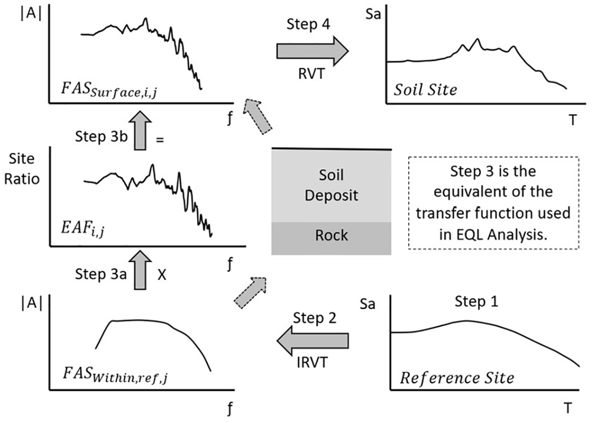
Process for using RVT and IRVT to utilize spectral amplifications to estimate site-specific response spectra given the response spectrum for a reference site. Step 1, the selection of the input response spectrum, begins in the lower right-hand corner. IRVT is performed in Step 2. Step 3 involves taking the FAS_Within developed in Step 2 and applying the Site Ratio using Equation 2 to calculate FAS_Surface. Step 3 is analogous to the process used in standard EQL analysis, where an input ground motion is applied at the bottom of the soil model and the output of the soil model is a surface spectrum (dashed arrows). Step 4 is to perform RVT to calculate the Soil Site response spectrum. T is the spectral period, Sa is spectral acceleration, and|A| is Fourier spectral amplitude.

Application of the proposed methodology

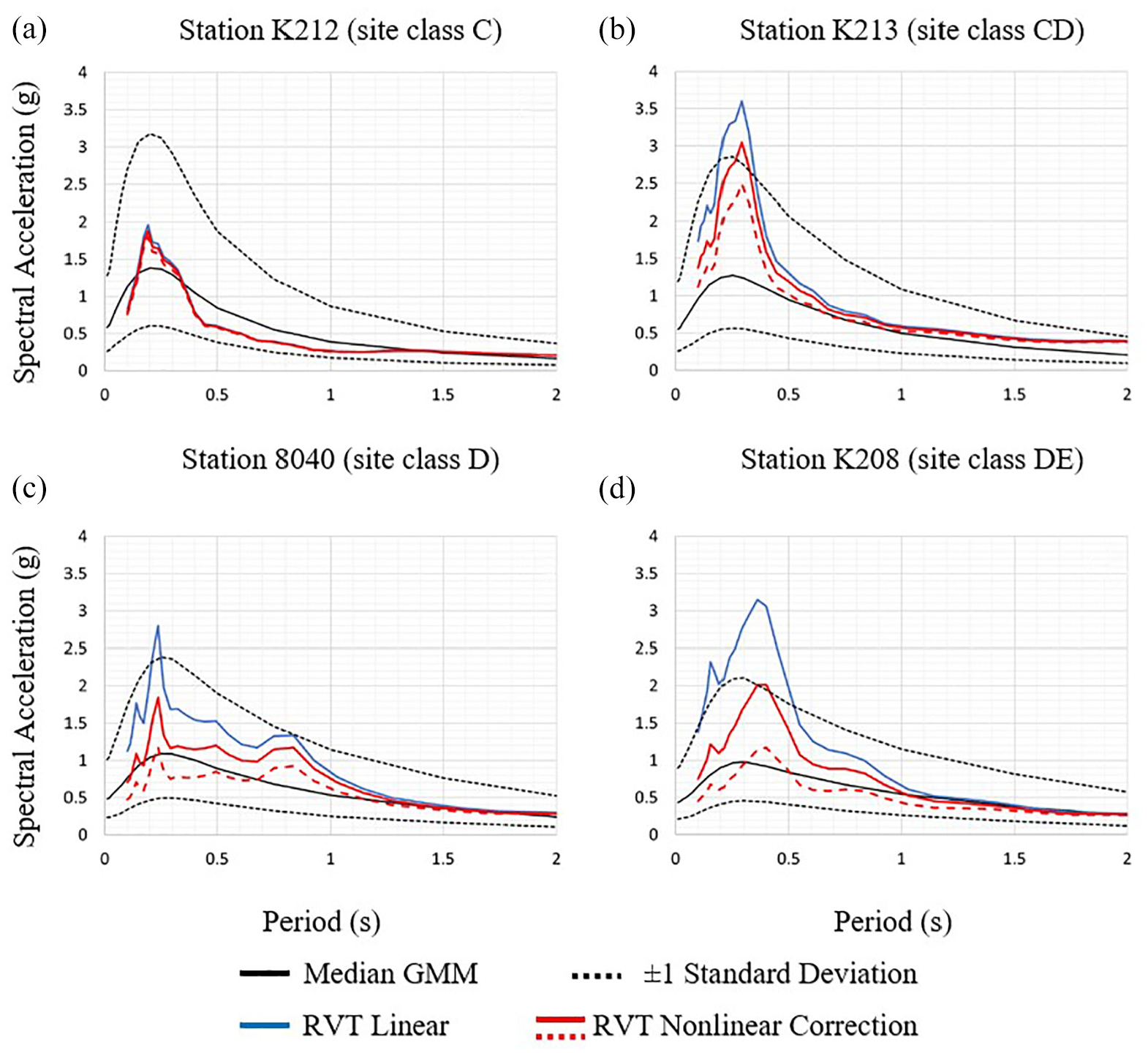
To test this methodology, ground motions recorded during the 2018 M_W 7.1 Anchorage Earthquake at Station K216 and several strong-motion stations in Anchorage are used. The orthogonal response spectra at Station K216 (Step 1) are converted to FAS using IRVT (Step 2). In this instance, the two orthogonal horizontal components were combined after performing IRVT using Equation 1. The GIT spectral amplifications for the event, also presented by Thornley et al. (2021a) for each site, are applied to the FAS (FAS_Within) at Station K216 to calculate each site’s FAS (FAS_Surface), as described in Step 3. Using RVT, the site FAS is converted to the response spectrum for the site (Step 4). It should be noted that there are several options to modify the duration, magnitude, damping, and other parameters in Strata. Provided, however, the user consistently uses the same parameters for IRVT and RVT calculations, the results achieved in Step 4 remain unaffected. The results are compared in Figure 5 to the response spectra calculated from the ground motions recorded at each site. This process was performed for several other earthquakes of lower magnitudes recorded in Anchorage, and similar good matches were achieved.

Figure 5.

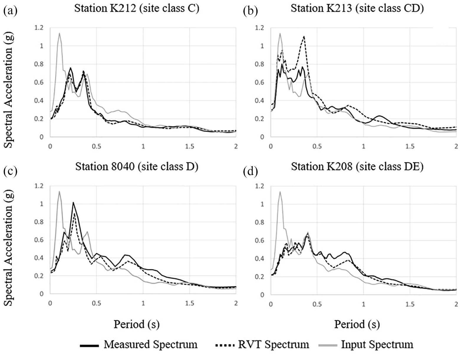
Measured and RVT-based response spectra for four strong-motion stations using the M_W 7.1 Anchorage earthquake. For reference, the grey line indicates the K216 (reference site) response spectrum. The stations represent stiffer (site class C) to softer sites (site class DE) in (a.) through (d.), respectively.

In general, the match between observed and the RVT approach response spectra is close, although not exact. The locations of the peaks and their amplitudes are generally similar. As an example, Station 8040 (Figure 5c) has a maximum difference of 39% at 1.3 s, but an average difference of less than 16%. Station K212 (Figure 5a) has a maximum difference of less than 20% with an average of 5%. These differences may be attributed to several reasons, including the potential effects of using the EAF (Equation 1) to combine the two orthogonal components.

To verify the appropriateness of the RVT-based approach, an evaluation was also performed to consider the results of the EAF (with frequency converted to period) applied directly to the reference site response spectrum without the use of RVT. A comparison of the measured response spectrum and the EAF-based response spectrum is presented in Figure 6. EAF-based response spectrum does not provide a reasonable fit, as there are several periods where the spectra differ by factors of two or more, which is supported by differences in FAS and response spectra (e.g. Bora et al., 2016). The RVT-based approach provides consistently similar results to the measured response spectra.

Figure 6.

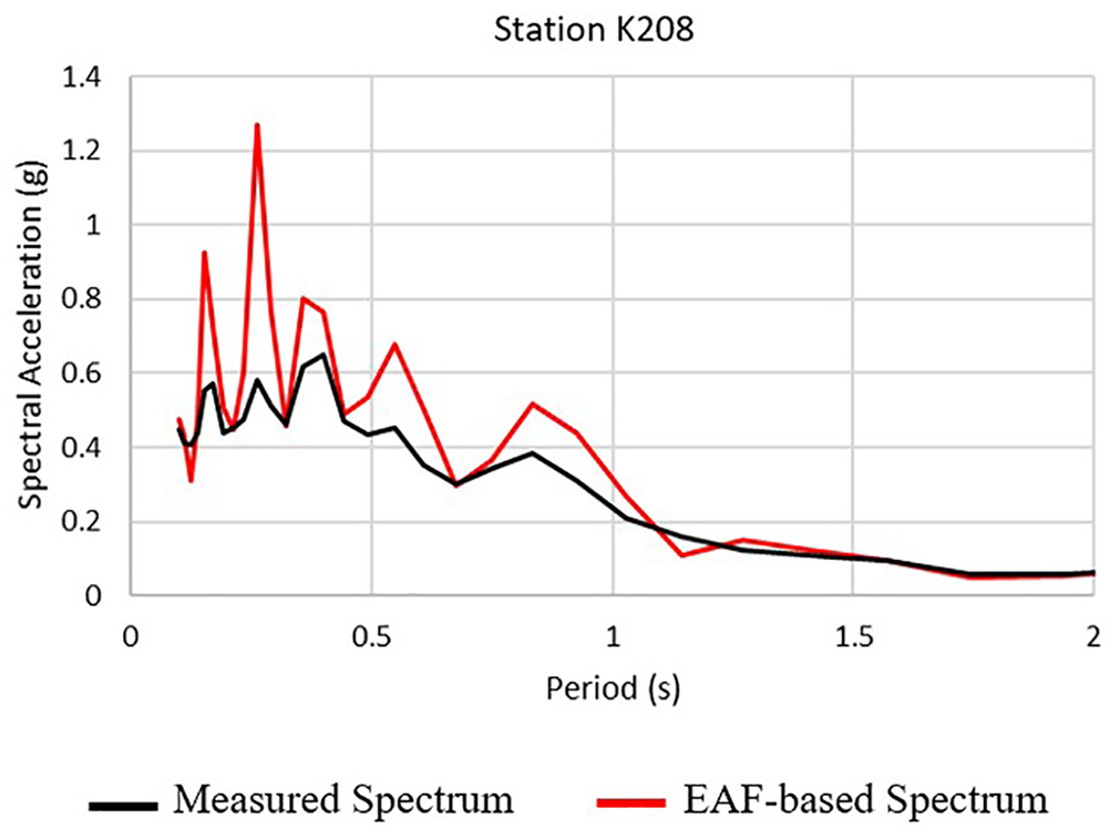
Measured and EAF-based response spectra at Station K208.

Nonlinear site effects

Nonlinear site response, due to the response of soil undergoing large strains, is an important aspect of any model for large earthquake ground motions. As described in Thornley et al. (2021a), the 2018 M_W 7.1 Anchorage Earthquake resulted in nonlinear site response at the strong-motion stations with lower V_S30. Numerous ground-motion models (GMMs) attempt to include both linear and nonlinear site responses. Several current GMMs do this by using the following equation:

F_{S} = \ln (F_{lin}) + \ln (F_{nl}),

(3)

where F_S is the site amplification; F_lin is the linear term of the site amplification as a result of small shear strain; and F_nl is the nonlinear term that accounts for the large shear strain response of the soil at the site. This combination of terms is discussed in Seyhan and Stewart (2014), Harmon et al. (2019), and Parker et al. (2020), among others.

As presented by Hashash et al. (2018), site response analyses within the western United States (WUS) show that the F_nl term has a greater impact on the response spectrum at periods less than 1 s. The impacts of nonlinear site response tend to affect softer sites (i.e. sites with smaller V_S30). Seyhan and Stewart (2014) found that the F_nl term has the largest impact at a period of approximately 0.3 s. As shown in subsequent sections, the F_nl term results in a reduction of the spectral accelerations for the Anchorage study, especially at sites in classes D and DE.

The response spectra for each station calculated by the RVT-based approach have been developed using numerous moderate-magnitude earthquakes. As suggested previously, only one or two events may have caused nonlinear response at some of the strong-motion stations. Due to their great epicentral distances and/or small magnitudes, the other events caused minor or no nonlinear site response at the stations evaluated. The spectral amplification used in this study is considered to be the F_lin term, as nonlinear effects were found, through a sensitivity analysis, to have an insignificant impact on the average site response (Thornley et al., 2021b). Accounting for potential nonlinearity using terms provided by Seyhan and Stewart (2014) will reduce the likelihood of overestimating short-period spectral accelerations using the RVT-based approach.

Comparison with EQL site response modeling

To further validate the RVT-based approach, the following section presents a comparison with the results of EQL analyses using selected earthquake ground motions. As mentioned previously, a calibrated EQL model has been developed for the DPDA. Four ground motions from shallow crustal earthquakes recorded at surface sites with V_S30 greater than 700 m/s were selected from the PEER (2021) database (Table 1) and are considered as reference sites recording large earthquakes for this study due to their V_S30 values. The response spectrum was calculated for each time history and utilized in Step 1 of the RVT-based analysis as the reference station, and the surface response for Station 8040 was calculated. The same time history was applied as an outcrop motion for use in the DPDA model. In addition to the F_lin response term, the RVT-based response spectrum was adjusted to account for F_nl, as described above.

The resulting response spectra for the RVT-based approach and the EQL analysis are presented in Figure 7. The input response spectrum for each event is also plotted to provide a comparison of input and output spectra. The model presented by Thornley et al. (2019) and Thornley et al. (2020) was not modified and the EAF, as presented in Thornley et al. (2021b), was used for the RVT-based approach. The results presented in Figure 7 show that the periods of the peaks match and that accounting for nonlinear effects reduces the spectral accelerations to better match the amplitude of the EQL results. Between periods of about 0.3 s and 0.6 s, the RVT-based model tends to overpredict the site response, when compared with the DPDA model. This may reflect the ground motions used to develop the EAF but is more likely related to more complex site response being captured by the RVT-based approach than can be captured by a 1-D EQL analysis. In addition to characteristics related to the ground motions, the maximum shear strain within the soil column and ground surface PGA are presented in Table 1. The shear strain index (I_γ), estimated by PGV_in/V_S30 (Idriss, 2011), is calculated to verify the appropriateness of the EQL model. Kim et al. (2016) found that EQL results with I_γ < 0.1% provide similar results to nonlinear analyses. The results in Figure 7c and d may be better approximated using a nonlinear model. However, for this study, the results show that the DPDA EQL model provides a similar response. The PGAs presented in Table 1 were used to calculate the nonlinear site modifications.

Figure 7.

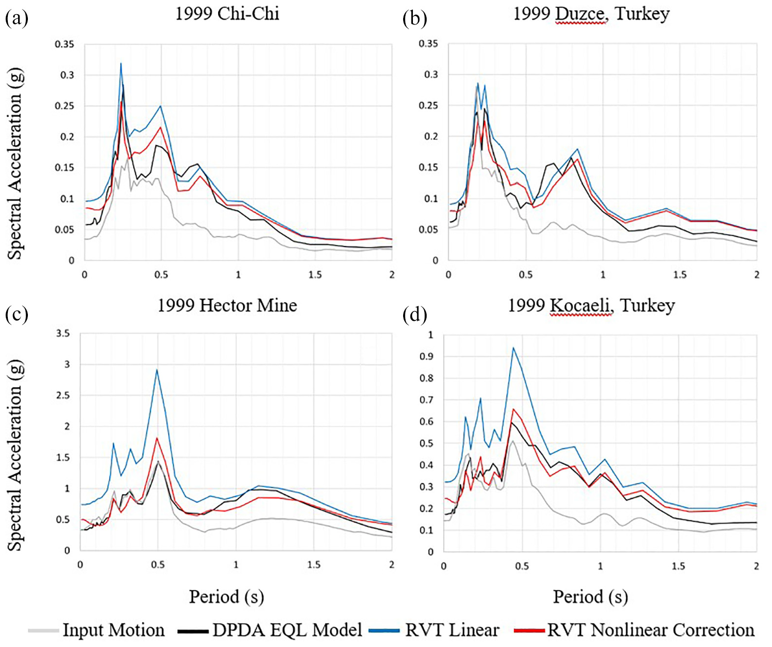
The results of the comparison between the DPDA EQL model and the RVT-based approach using the four records presented in Table 1 as input motions. The results using the 1999 Chi-chi event are shown in (a.), 1999 Duzce, Turkey event in (b.), 1999, Hector Mine in (c.), and the 1999 Kocaeli, Turkey event in (d.). Note the change in vertical scale in (c.) and (d.).

Ground motion model comparison

With the validation of the RVT-based technique for local earthquakes and as a substitute for EQL analyses, a logical next step is to consider further application of the method. Recently, two Next Generation Attenuation Subduction (NGA-Sub) GMMs were released by Parker et al. (2020) and Kuehn et al. (2020). Because of the proximity of Anchorage to the subduction zone, the high rate of earthquake activity, and the likelihood of damaging earthquakes, subduction interface earthquakes account for 36% of the earthquake hazard for Anchorage, according to the disaggregated hazard of the “Dynamic: Alaska 2007 (v2.1.2)” hazard model presented by USGS.gov (2021). This model indicates a M_W 9.2 interface earthquake at a rupture depth (r_RUP) of 36 km as the modal scenario. Using this earthquake as a test case, site response spectra estimated using the NGA-Sub GMMs are compared here to response spectra using the RVT-based technique.

The NGA-Sub hazard characterization tool (Mazzoni, 2020) was used to calculate the response spectrum for the site class BC, where the V_S30 is 760 m/s, and the estimated V_S30 values were used at the strong-motion stations. The Parker et al. (2020) and Kuehn et al. (2020) models (Global variants) were equally weighted. The site class BC response spectrum was used in Step 1 (Figure 4) as the reference site response spectra. The EAF_{i, j} for each station (Step 3) was used to calculate the soil site response spectra. The PGA estimated by the GMMs is then used to calculate F_nl using the approach presented by Parker et al. (2020) and the soil site response spectra are adjusted to account for nonlinear site response. The comparison between the two approaches is presented in Figure 8.

Figure 8.

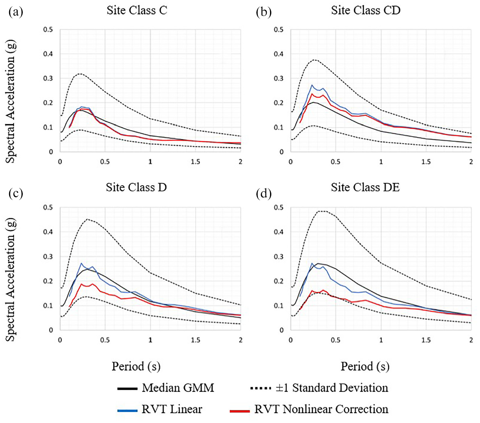
Response spectra for the NGA-Sub GMMs for the M_W 9.2 event. The solid red line corrects for nonlinearity using the factors recommended by Parker et al. (2020) and the dashed red lines using the factors of Seyhan and Stewart (2014). The results show a range of site response values from the stiffer (site class C) site in (a.) through a softer site (site class DE) in (d.).

The results indicate that the RVT technique provides similar results to the NGA-Sub estimates, but the proposed technique provides additional site-specific details related to amplification behavior at each site. Utilizing the nonlinear modification, the RVT-based spectral accelerations are reduced at shorter periods and the shapes of the overall spectra are similar to those estimated by NGA-Sub. Even when the nonlinear response is accounted for, the site-specific response spectra tend to be above the median GMM estimate for periods below 1 s. However, the response spectra are within one standard deviation of the median, indicating a reasonable match. Modification of the factors utilized in the calculation of F_nl may help improve the fit. Figure 8 shows the differences when using F_nl factors recommended by Parker et al. (2020) and Seyhan and Stewart (2014), indicated by the solid red lines and dashed red lines, respectively. A fit closer to the NGA-Sub GMM median values is achieved using the Seyhan and Stewart (2014)F_nl term, especially at softer sites (i.e. site class D and DE).

The EAF results from the strong-motion stations were also divided by site class (defined by V_S30 estimated by Thornley et al., 2021c). The range of response spectra for the strong-motion stations, divided by site class, is presented in Figure 9 along with the median and ±1 standard deviation (shaded region) spectra. The response spectra in Figure 9 have not been adjusted to account for possible nonlinear site effects.

Figure 9.

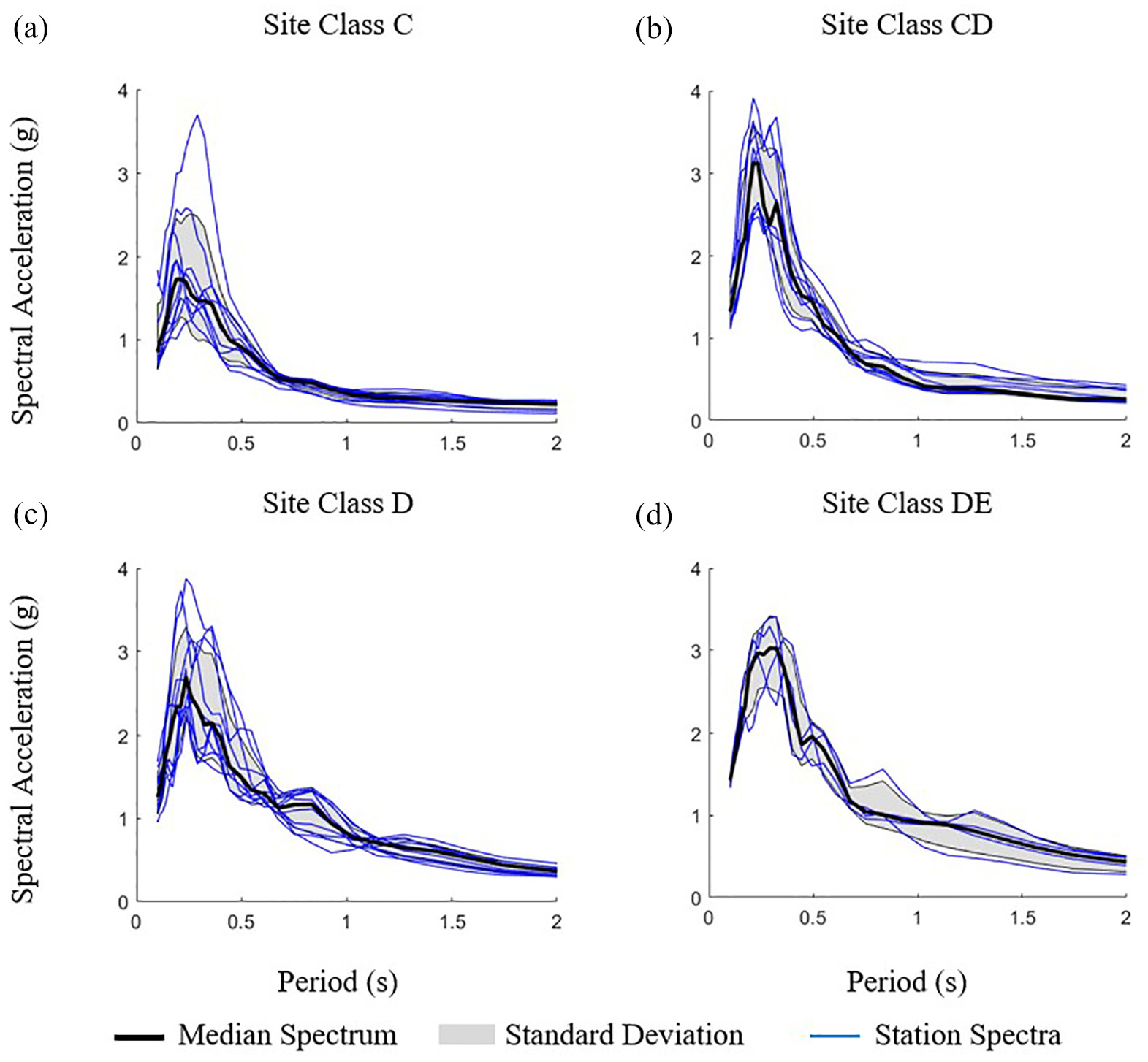
Response spectra for strong-motion stations in Anchorage by site class. A range of results for different site classes are shown, with Site Class C (a.), Site Class CD (b.), Site Class C (c.), and Site Class DE (d.).

The average EAF for each site class was then used to estimate an average response spectrum for each site class similar to the process described above. The average V_S30 for each site class was used to calculate the NGA-Sub GMM response spectra (Table 2). The results for the four site classes are presented in Figure 10. The Seyhan and Stewart (2014) nonlinear adjustment provides a closer fit between the site class response spectra and the NGA-Sub GMM response spectra.

Table 2.

V_S30 ranges by site class proposed by BSSC (2019) and Anchorage strong-motion station estimates used in this study

Site Class	V_S30 Range(BSSC 2020) (m/s)	Strong-motionStation V_S30Range (m/s)	Strong-motionStation V_S30Average (m/s)	Number of Strong-motionStations
C	440 – 640	465 – 594	516	10
CD	300 – 440	315 – 439	376	9
D	215 – 300	224 – 285	244	10
DE	150 – 215	167 – 213	196	4

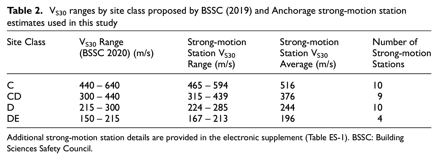
Additional strong-motion station details are provided in the electronic supplement (Table ES-1). BSSC: Building Sciences Safety Council.

Figure 10.

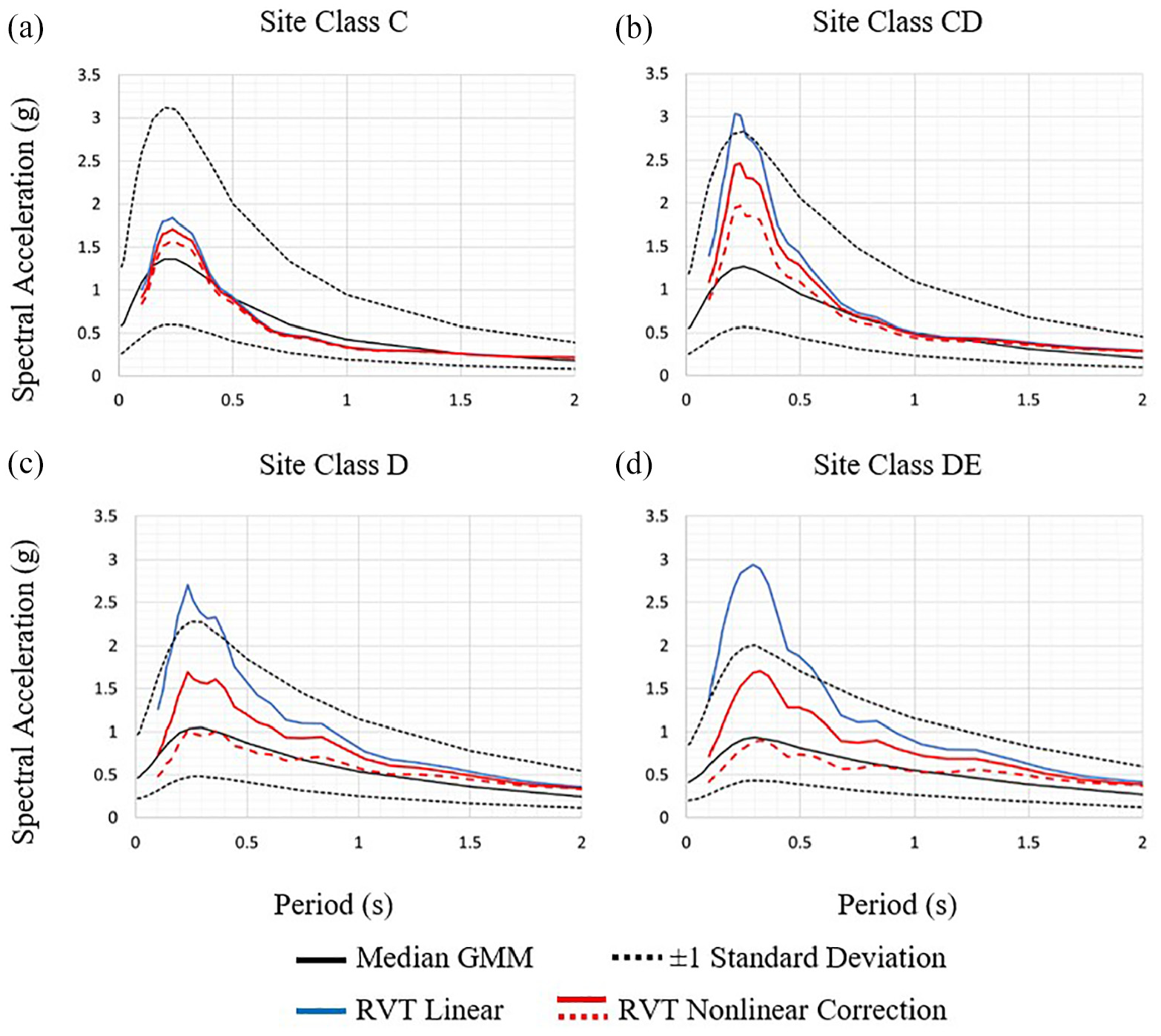
Median response spectra for the combination of strong-motion stations in Anchorage by site class comparing the NGA Sub GMMs for the M_W 9.2 event and the RVT-based approach. A range of results for different site classes are shown, with Site Class C (a.), Site Class CD (b.), Site Class C (c.), and Site Class DE (d.). The solid red line corrects for nonlinearity using the factors recommended by Parker et al. (2020) and the dashed red line for Seyhan and Stewart (2014).

Crustal earthquake sources have also been included in the Alaska hazard model. The Castle Mountain Fault, north of Anchorage (Figure 1), is estimated to be able to produce strike-slip events up to M_W 7.5 (Wesson et al., 2007). This scenario earthquake was used to compare the results of the four equally weighted soil site NGA-West2 GMMs (Abrahamson et al., 2014; Boore et al., 2014; Campbell and Bozorgnia, 2014; Chiou and Youngs, 2014) and the RVT technique. This is evaluated in a similar fashion to the site class approach presented above. The F_nl term is developed using the factors suggested by Seyhan and Stewart (2014) for crustal earthquakes. The results of this comparison are provided in Figure 11. As shown previously, the nonlinear effect is minimal for site classes C and CD (Figure 11a and 11b) and the general shape of the spectral accelerations matches well with the shape and amplitude of the median NGA-West2 spectra. Figure 11c and 11d show the nonlinear effects for a M_W 7.5 crustal earthquake 65 km from Anchorage may not be as prevalent as suggested by the substantial reduction in spectral accelerations at shorter periods and the nonlinear term may not be appropriate when crustal earthquakes at greater distances are used.

Figure 11.

Median response Spectra for the combination of Anchorage site classes comparing the NGA-West2 GMMs for the M_W 7.5 event and the RVT-based approach. A range of results for different site classes are shown, with Site Class C (a.), Site Class CD (b.), Site Class C (c.), and Site Class DE (d.).

Discussion and application

One of the limitations of microzonation studies is the need for proper engineering characterization of the subsurface soil, especially at strong-motion stations, to draw conclusions about sites within the vicinity that have similar subsurface conditions. As described here, the Anchorage strong-motion network does not have this level of characterization. Still, unlike regional strong-motion networks, such as in the central and eastern United States (CEUS), the Anchorage network has recorded numerous moderate to strong earthquakes. The use of RVT techniques with GIT-derived spectral amplification allows the characterization of site response without additional subsurface characterization, as shown in Figure 5. This is especially beneficial because even with the proper characterization of subsurface conditions, the selection of shear modulus reduction and damping curves can have a significant impact on the results of EQL analyses.

As mentioned previously, one of the benefits of the use of spectral amplification measured at the strong-motion stations is that the site response, especially in the linear range, is accounted for in the results. This is beneficial when performing site response analysis, whether EQL or nonlinear. The results allow for calibration of site models under small strain before extending those models to the nonlinear realm. This can also support a methodology for selecting and applying shear modulus reduction and damping curves for regional soil types so that a model for a strong-motion station can be applied to other sites within a region. A limitation of this method is that it requires several recordings from numerous strong-motion stations to obtain stable results, and a new construction does not necessarily have a corresponding strong-motion station. However, for microzonation studies, which have utilized EQL in the past, this methodology may provide additional insight into the variations in regional site response and its characterization.

When utilizing the RVT-based methodology, several aspects should be considered. As presented in Kottke et al. (2019), care should be taken when calculating input FAS from response spectra. Reference site response spectra may need to be upsampled to achieve appropriate FAS representation. In addition, unlike GMM applications using RVT, parameters such as magnitude, duration, and other modifications do not need to be accounted for in this method, provided that the parameters used in Step 2 and Step 4 (Figure 4) are the same. The results of GIT provide standard error estimates, which can be utilized to evaluate the uncertainty of results for future studies. Finally, the spectral amplification used in this study resulted primarily from smaller-magnitude earthquakes that provide linear site response, allowing for the subsequent application of the F_nl term. Care should be given to the selection of earthquakes for the GIT analysis so that nonlinear response is not accounted for twice. On the other hand, if the ground motions used in the GIT analysis already account for nonlinear response (Figure 4) then F_nl may not need to be applied.

Conclusions

The use of Fourier spectral amplification results directly in geotechnical engineering studies has been limited. This is because there has been no coherent and simple approach to transfer the Fourier spectral amplification results to the response spectral-domain more common in engineering studies. The methodology presented in this study provides the opportunity to directly utilize Fourier spectral amplification to estimate response spectra for strong-motion stations without the need for engineering characterization of subsurface conditions. The methodology, shown here to be compatible with individual earthquakes, can be extended to incorporate the results from numerous earthquakes to capture average site response. While the initial results provide the linear response, applying a nonlinear term allows for the correction of site response to include nonlinear effects on the response spectrum.

Supplemental Material

sj-pdf-1-eqs-10.1177_87552930211065482 – Supplemental material for Engineering site response analysis of Anchorage, Alaska, using site amplifications and random vibration theory

Supplemental material, sj-pdf-1-eqs-10.1177_87552930211065482 for Engineering site response analysis of Anchorage, Alaska, using site amplifications and random vibration theory by John Thornley, John Douglas, Utpal Dutta and Zhaohui (Joey) Yang in Earthquake Spectra

Footnotes

Acknowledgements

The authors thank the staff at Alaska Earthquake Center (AEC), especially Natalia Ruppert, Mike West, and Mitch Robinson, for providing the majority of data for this study. The United States Geological Survey (USGS) and AEC should also be thanked for maintaining the Anchorage strong-motion stations. Many thanks are owed to Jamie Steidl and his team at the University of California Santa Barbara for their efforts to maintain the Delaney Park Downhole Array and the data collected there. Albert Kottke of Pacific Gas & Electric Company and his efforts to continue to develop the computer program Strata, along with helpful correspondence and his thoughtful review of the manuscript, have been very helpful for this study. James Kaklamanos also provided a detailed review of the manuscript and gave thoughtful and helpful comments that have greatly improved the article.

Data resources

The earthquake records utilized in this study were provided by the AEC or downloaded from IRIS (https://www.iris.edu/hq/) and University of California Santa Barbara (http://www.nees.ucsb.edu/). ESRI ArcMap 10.6.1 was used to develop Figures 1 and 2. The GIT analysis and most of the remaining figures were generated using GITANES (Klin, 2019) in MATLAB and scripts created in MATLAB by the authors. RVT analysis was performed using Strata (Kottke and Rathje, 2008).

Declaration of conflicting interests

The author(s) declared no potential conflicts of interest with respect to the research, authorship, and/or publication of this article.

Funding

The author(s) received no financial support for the research, authorship, and/or publication of this article.

Supplemental material

Supplemental material for this article is available online.

References

Abrahamson

Silva

Kamai

(2014) Summary of the ASK14 ground motion relation for active crustal regions. Earthquake Spectra 30(3): 1025–1055.

Alaska Earthquake Center (AEC) (2021) Available at: https://earthquake.alaska.edu/earthquakes/about (accessed 6 February 2021).

Andrews

(1986) Objective determination of source parameters and similarity of earthquakes of different size. In: Das

Boatwright

Scholz

(eds) Earthquake Source Mechanics (American Geophysical Monograph 37, vol. 6). Washington, DC: AGU, pp. 259–267.

Bayless

Abrahamson

(2019) An empirical model for the interfrequency correlation of epsilon for Fourier amplitude spectra. Bulletin of the Seismological Society of America 109(3): 1058–1070.

Bindi

Spallarossa

Pacor

(2017) Between-event and between-station variability observed in the Fourier and response spectra domains: Comparison with seismological models. Geophysical Journal International 210: 1092–1104.

Boore

(1983) Stochastic simulation of high-frequency ground motions based on seismological models of the radiated spectra. Bulletin of the Seismological Society of America 73(6): 1865–1894.

Boore

(2003) Simulation of ground motion using the stochastic method. Pure and Applied Geophysics 160(3–4): 635–676.

Boore

Joyner

(1984) A note on the use of random vibration theory to predict peak amplitudes of transient signals. Bulletin of the Seismological Society of America 74(5): 2035–2039.

Boore

Stewart

Seyhan

Atkinson

(2014) NGA-West2 equations for predicting PGA, PGV, and 5% damped PSA for shallow crustal earthquakes. Earthquake Spectra 30(3): 1057–1085.

10.

Bora

Scherbaum

Kuehn

Stafford

(2016) On the relationship between Fourier and response spectra: Implications for the adjustment of empirical ground-motion prediction equations (GMPEs). Bulletin of the Seismological Society of America 106(3): 1235–1253.

11.

Borcherdt

(1970) Effects of local geology on ground motion near San Francisco Bay. Bulletin of the Seismological Society of America 60(1): 29–61.

12.

Building Sciences Safety Council (BSSC) (2019) BSSC Project Final Report: Development of the Next Generation of Seismic Design Value Maps for the 2020 NEHRP Provisions. Washington, DC: National Institute of Building Sciences.

13.

Campbell

Bozorgnia

(2014) NGA-West2 ground motion model for the average horizontal components of PGA, PGV, and 5% damped linear acceleration response spectra. Earthquake Spectra 30(3): 1087–1115.

14.

Chiou

BS-J

Youngs

(2014) Update of the Chiou and Youngs NGA model for the average horizontal component of peak ground motion and response spectra. Earthquake Spectra 30(3): 1117–1153.

15.

Combellick

(1999) Simplified geologic map and cross sections of central and east Anchorage, Alaska. Preliminary interpretive report 1999-1. Fairbanks, AK: Alaska Division of Geological & Geophysical Surveys.

16.

Dutta

Biswas

Martirosyan

Papageorgiou

Kinoshita

(2003) Estimation of earthquake source parameters and site response in Anchorage, Alaska from strong-motion network data using generalized inversion method. Physics of the Planetary Interiors 137: 13–29.

17.

Ghofrani

Atkinson

(2014) Site condition evaluation using horizontal-to-vertical response spectral ratios of earthquakes in the NGA-West 2 and Japanese databases. Soil Dynamics and Earthquake Engineering 67: 30–43.

18.

Haeussler

(2008) An overview of the neotectonics of interior Alaska: Far-field deformation from the Yakutat microplate collision. In: Freymueller

Haeussler

Wesson

Ekström

(eds) Active Tectonics and Seismic Potential in Alaska (Geophysics Monograph Series, vol. 179). Washington, DC: American Geophysical Union, pp. 83–108.

19.

Hanks

McGuire

(1981) The character of high-frequency strong ground motion. Bulletin of the Seismological Society of America 71(6): 2071–2095.

20.

Hansen

(1965) Effects of the earthquake of March 27, 1964, at Anchorage, Alaska. U.S. Geological Survey Professional Paper (542-A). Menlo Park, CA: U.S. Geological Survey, 68 pp.

21.

Harmon

Hashash

YMA

Stewart

Rathje

Campbell

Silva

Ilhan

(2019) Site amplification functions for Central and Eastern North America—Part II: Modular simulation-based models. Earthquake Spectra 35(2): 815–847.

22.

Hashash

YMA

Dashti

Romero

Ghayoomi

Musgrove

(2015) Evaluation of 1-D seismic site response modeling of sand using centrifuge experiments. Soil Dynamics and Earthquake Engineering 78: 19–31.

23.

Hashash

YMA

Harmin

Ilhan

Stewart

Rathje

Campbell

Silva

Goulet

(2018) Modelling of site amplifications via large scale nonlinear simulations with applications to North America. Geotechnical Earthquake Engineering and Soil Dynamics V, GSP 291. Reston, VA: American Society of Civil Engineers.

24.

Hayes

(2018) Slab2—A comprehensive subduction zone geometry model. U.S. Geological Survey data release. DOI: 10.5066/F7PV6JNV.

25.

Idriss

(2011) Use of Vs30 to represent local site conditions. In: 4th LASPEI/IAEE international symposium effects of surface geology on strong ground motions, Santa Barbara, CA, 23–26 August.

26.

Idriss

Sun

(1992) Shake91: A computer program for conducting equivalent linear seismic response analysis of horizontally layered soil deposits. User’s Guide, Center for Geotechnical Modeling, Civil Engineering Department, UC Davis, Davis, CA.

27.

Kim

Hashash

Stewart

Rathje

Harmon

Musgrove

Campbel

Silva

(2016) Relative differences between nonlinear and equivalent-linear 1-D site response analyses. Earthquake Spectra 32(3): 1845–1865.

28.

Klin

(2019) GITANES. MATLAB Central File Exchange. Available at: https://www.mathworks.com/matlabcentral/fileexchange/61711-gitanes (accessed August 15, 2019).

29.

Koehler

(2013) Quaternary Faults and Folds (QFF). Digital Data Series 3. Fairbanks, AK: Alaska Division of Geological & Geophysical Surveys (Koehler RD, Burns PAC and Weakland JR, 2013, Digitized faults of the Neotectonic map of Alaska (Plafker and others, 1994), in Koehler RD. Quaternary Faults and Folds (QFF): Alaska Division of Geological & Geophysical Surveys Miscellaneous Publication 150, p. 1).

30.

Kottke

Rathje

(2008) Technical manual for Strata. Report No. 2008/10. Berkeley, CA: Pacific Earthquake Engineering Research Center, University of California, Berkeley.

31.

Kottke

Wang

Rathje

(2019) Strata technical manual. Available at: https://github.com/arkottke/strata (accessed 24 January 2021).

32.

Kuehn

Bozorgnia

Campbell

Gregor

(2020) Partially non-ergodic ground-motion model for subduction regions using the NGA-subduction database. Report No. 2020/04, September. Berkeley, CA: Pacific Earthquake Engineering Research Center, University of California, Berkeley.

33.

Laurenzano

Barnaba

Romano

Priolo

Bertoni

Bragato

Comelli

Dreossi

Garbin

(2019) The Central Italy 2016–2017 seismic sequence: Site response analysis based on seismological data in the Arquata del Tronto–Montegallo municipalities. Bulletin of Earthquake Engineering 17: 5449–5469.

34.

Mazzoni

(2020) NGA-subduction ground-motion characterization tool, June. Available at: https://www.risksciences.ucla.edu/nhr3/gmtools?rq=NGA%20Subduction (accessed September 2020).

35.

National Academies of Sciences Engineering and Medicine (NASEM) (2012) Practices and Procedures for Site-Specific Evaluations of Earthquake Ground Motions. Washington, DC: The National Academies Press.

36.

Oth

Parolai

Bindi

Wenzel

(2009) Source spectra and site response from S waves of intermediate-depth Vrancea, Romania, Earthquakes. Bulletin of the Seismological Society of America 99(1): 235–254.

37.

Parker

Stewart

Boore

Atkinson

Hassani

(2020) NGA-subduction global ground-motion models with regional adjustment factors. Report No: 2020/03. Berkeley, CA: Pacific Earthquake Engineering Research Center, University of California, Berkeley.

38.

Parolai

Bindi

Augliera

(2000) Application of the generalized inversion technique (GIT)to a microzonation study: Numerical simulations and comparison with different site-estimation techniques. Bulletin of the Seismological Society of America 90(2): 286–297.

39.

PEER (2021) PEER 2013/03—PEER NGA-West2 database web portal (Ancheta TD, Darragh RB, Stewart JP, Seyhan E, Silva WJ, Chiou BSJ, Wooddell KE, Graves RW, Kottke AR, Boore DM, Kishida T and Donahue JL). Available at: https://ngawest2.berkeley.edu/spectras/new?sourceDb_flag=1 (accessed May 27, 2021).

40.

Rathje

Kottke

(2008) Procedures for random vibration theory based seismic site response analyses: A white paper prepared for the nuclear regulatory commission. Geotechnical Engineering Report GR08-09. Austin, TX: Geotechnical Engineering Center, Department of Civil, Architectural, and Environmental Engineering, University of Texas at Austin.

41.

Régnier

Bonilla

Bard

Bertrand

Hollender

Kawase

Sicilia

Arduino

Amorosi

Asimaki

Boldini

Chen

Chiaradonna

DeMartin

Elgamal

Falcone

Foerster

Foti

Garini

Gazetas

Gélis

Ghofrani

Giannakou

Gingery

Glinsky

Harmon

Hashash

Iai

Kramer

Kontoe

Kristek

Lanzo

di Lernia

Lopez-Caballero

Marot

McAllister

Diego Mercerat

Moczo

Montoya-Noguera

Musgrove

Nieto-Ferro

Pagliaroli

Passeri

Richterova

Sajana

Paola Santisi d’Avila

Shi

Silvestri

Taiebat

Tropeano

Vandeputte

Verrucci

(2018) PRENOLIN: International Benchmark on 1D Nonlinear Site Response Analysis—Validation Phase Exercise. Bulletin of the Seismological Society of America 108 (2): 876–900.

42.

Seyhan

Stewart

(2014) Semi-empirical nonlinear site amplification from NGA-West2 data and simulations. Earthquake Spectra 30(3): 1241–1256.

43.

Stewart

Afshari

Hashash

YMA

(2014) Guidelines for performing hazard-consistent one-dimensional ground response analysis for ground motion prediction. Report 2014/16, October. Berkeley, CA: Pacific Earthquake Engineering Research Center.

44.

Thornley

Dutta

Fahringer

Yang

(2019) In situ shear-wave velocity measurements at the Delaney Park Downhole Array, Anchorage, Alaska. Seismological Research Letters 90(1): 395–400.

45.

Thornley

Dutta

Douglas

Yang

(2021a) Nonlinear site effects from the 30 November 2018 Anchorage, Alaska, earthquake. Bulletin of the Seismological Society of America 2021; 111: 2112–2120.

46.

Thornley

Douglas

Dutta

Yang

(2021b) Site response analysis of Anchorage, Alaska using generalized inversions of strong-motion data (2014-2019). Pure and Applied Geophysics (In Review).

47.

Thornley

Dutta

Douglas

Yang

(2021c) Evaluation of horizontal to vertical spectral ratio and standard spectral ratio methods for mapping shear wave velocity across Anchorage, Alaska. Soil Dynamics and Earthquake Engineering 150(2021): 106918.

48.

Thornley

Dutta

Yang

Douglas

(2020) Nonlinear site response analysis at the Delaney Park Downhole Array in Anchorage, Alaska. In: 17th world conference on earthquake engineering, Paper Number C004020. Sendai, Japan (September 27, 2021).

49.

Ulery

Updike

(1983) Subsurface structure of the cohesive facies of the Bootlegger Cove formation, southwest Anchorage. Alaska Division of Geological & Geophysical Surveys Professional Report 84, 3 sheets, scale 1:15,840. DOI: 10.14509/2257.

50.

Updike

Ulery

(1986) Engineering-geologic map of Southwest Anchorage, Alaska. Alaska Division of Geological and Geophysical Surveys Professional Report 89, sheet 1 of 1. DOI: 10.14509/2270.

51.

USGS.gov (2020) M9.2 Alaska Earthquake and Tsunami ofMarch 27, 1964. Available at: https://earthquake.usgs.gov/earthquakes/events/alaska1964/ (accessed 30 May 2020).

52.

USGS.gov (2021) Unified hazard tool. Available at: https://earthquake.usgs.gov/hazards/interactive/ (accessed 1 May 2021).

53.

Wesson

Boyd

Mueller

Bufe

Frankel

Petersen

(2007) Revision of time-independent probabilistic seismic hazard maps for Alaska. U.S. Geological Survey Open-File Report 2007-1043. Reston, VA: U.S. Geological Survey.

54.

West

Bender

Gardine

Gately

Haeussler

Hassan

Meyer

Richards

Ruppert

Tape

Thornley

Witter

(2020) The 30 November 2018 Mw 7.1 Anchorage Earthquake. Seismological Research Letters 91(1): 66–84.

55.

Wilson

Hults

Schmoll

Haeussler

(2012) Geologic map of the Cook Inlet region, Alaska, including parts of the Talkeetna, Talkeetna Mountains, Tyonek, Anchorage, Lake Clark, Kenai, Seward, Iliamna, Seldovia, Mount Katmai, and Afognak 1:250,000-scale quadrangles. Reston, VA: U.S. Geological Survey, pp. i-71.

Supplementary Material

Please find the following supplemental material available below.

For Open Access articles published under a Creative Commons License, all supplemental material carries the same license as the article it is associated with.

For non-Open Access articles published, all supplemental material carries a non-exclusive license, and permission requests for re-use of supplemental material or any part of supplemental material shall be sent directly to the copyright owner as specified in the copyright notice associated with the article.

0.00 MB

0.06 MB

Engineering site response analysis of Anchorage,Alaska,using site amplifications and random vibration theory

Abstract

Keywords

Introduction

Tectonic setting and seismicity

Geology

Strong-motion stations and data set

Site spectral amplification evaluation

Engineering site response using random vibration theory

Proposed methodology

Generalized approach

Application of the proposed methodology

Nonlinear site effects

Comparison with EQL site response modeling

Ground motion model comparison

Discussion and application

Conclusions

Supplemental Material

sj-pdf-1-eqs-10.1177_87552930211065482 – Supplemental material for Engineering site response analysis of Anchorage, Alaska, using site amplifications and random vibration theory

Footnotes

Acknowledgements

Data resources

Declaration of conflicting interests

Funding

Supplemental material

References

Supplementary Material