Sage Journals: Discover world-class research

Abstract

This article covers the impact of soil initial stress field heterogeneity (ISFH) in wave-passage analysis and in prescribed structural acceleration in the context of dynamic soil–structure interaction (DSSI) analysis. ISFH is directly related to the natural behavior of soil where a significant increase in net effective confinement, as is the case in the foundation soil under a building, tends to increase the soil’s modulus and strain. This creates a heterogeneous stress field in the vicinity of the foundation elements, which results in a modification of the dynamic behavior of the soil–structure system. A simple method for considering the impact of ISFH on the value of the soil’s modulus and strain was developed using the direct DSSI approach. The method was used to analyze numerical artifacts and its impact on the surface acceleration values of a nonlinear two-dimensional (2D) numerical soil deposit under transient loading. This analysis was followed by a sample application for a three-story, three-bay concrete moment-resisting frame structure erected on a deep soil deposit. Floor acceleration and relative displacement were used for comparison. The soil deposit was modeled using the typical geotechnical properties of fine-grained, post-glacial soil samples obtained in Eastern Canada from in situ geotechnical borehole drilling, geophysical surveys, and laboratory testing. Ground motion was based on eastern calibrated seismic signals. The results of the soil deposit analysis show that ISFH had a significant impact on surface acceleration values. The effect was found to be period-dependent and to have a direct impact on prescribed acceleration values at the base of structure. Thus, failure to take the effects of ISFH into consideration can lead to errors in calculating prescribed structural accelerations (i.e. over- or underestimation).

Keywords

Dynamic soil–structure interaction direct modeling finite element Eastern Canada post-glacial deposits

Introduction

We have long known that the dynamic behavior of a structure is largely influenced by site effects during an earthquake (Reid, 1906). The first documented work in North America that provided a better understanding of this phenomenon was carried out by Rogers (1906) in the aftermath of the California earthquake of 1906, when it was observed that “the character of the foundation was a far more potent factor in determining the damage done than nearness to the fault line” (Reid, 1906: 49). The same observation was made in 1985, when the soft soil beneath Mexico City amplified the ground motion of the Michoacán earthquake and caused severe damage to many structures (Mitchell et al., 1986). More recent experimental work (Gajan and Kutter, 2008) and post-event reports (Avilès and Pérez-Rocha, 1998; Cubrinovski et al., 2011) made it clear that site effects, including dynamic soil–structure interaction (DSSI) (Stewart et al., 1999), play a major role in the dynamic response of a structure. This is particularly true for rigid structures built on deep, loose soil deposits (Stewart et al., 2012).

One common method for modeling DSSI is to use the simplified substructure approach (Kausel et al., 1978; Lysmer et al., 1975), which is based on the superposition principle for linear systems. This method involves analyzing the effects of so-called kinematic and inertial interactions using two separate models. Analyzing kinematic interactions in the time domain consists in examining wave propagation in the soil column, where massless structural foundation elements are included in the model, to obtain the foundation input motion ( $u_{fim}$ ). The $u_{fim}$ is then used in an inertial interaction analysis in which the complete structural model is considered and soil effects (flexibility and damping) are examined using the appropriate elements at the soil–foundation interface (spring and dashpot in the time domain). A key element that is seldom considered in the kinematic interaction analysis phase is the total impact of net increases in effective confining stress on supporting soil behavior due to the transferred structural load, which we refer to in this article as initial stress field heterogeneity (ISFH) and which has two major effects.

The first effect is related to the soil moduli, which are known to be influenced by the level of confinement (Hardin and Black, 1968). This aspect is usually accounted for by imposing proper loads on a static soil model and calculating the increases in the soil moduli (shear, bulk, and Young’s) caused by the net increases in confining stress (Stewart et al., 2012). The values of the moduli are then recorded and serve as input in the dynamic soil model used to conduct the kinematic interaction analysis, where no structural loads from the structure are otherwise considered. In doing so, the initial state of confining stress associated with the moduli calculated in the first static soil model is not preserved in the kinematic analysis phase. This results in a kinematic interaction analysis where the soil moduli values are based on computation using the state of stress under the structural loads, while the actual state of stress in the model is that of the free field.

The second effect is related to the spatial distribution of the vertical load transferred from the structure. Because all footings have finite dimensions (B), loads from the structure are transferred to specific areas of the supporting soil, thus creating an anisotropic stress distribution within the soil’s elements. Consider the case of a single footing of width B, where net increases in the confining stress due to loads from the structure can be assumed to be bulb-shaped (Figure 1; Boussinesq, 1885).

Figure 1.

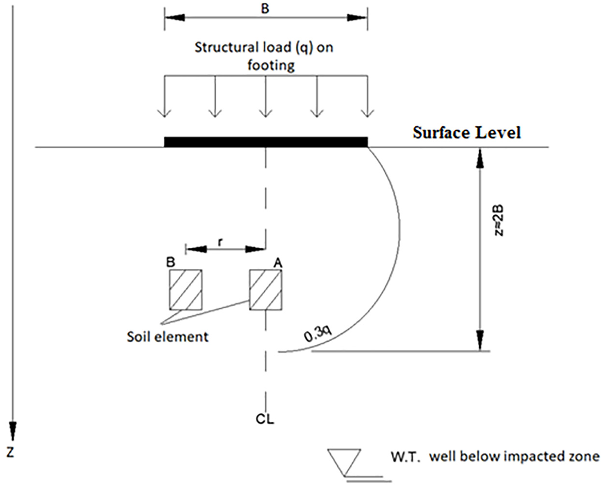
Transfer of structural load to supporting soil.

Before any structure is erected at a site under free-field conditions, the state of stress for elements at depth Z = B is shown in Figure 2a, where the ratio between the initial effective vertical and horizontal stress can be estimated using Jâky’s (1944) relation. Once the structure is built, structural load is transferred to the supporting soil, and the soil element centered under the footing (element A) is anisotropically consolidated beneath the structural load (Figure 2b). In the case of elements located at distance r from the center line (element B), the net increases in vertical stress are not symmetrical and can be depicted as triangular loading, as shown in Figure 2c, which indicates that the main stress axis is rotating as it generates a certain level of shearing stress on the vertical and horizontal planes.

Figure 2.

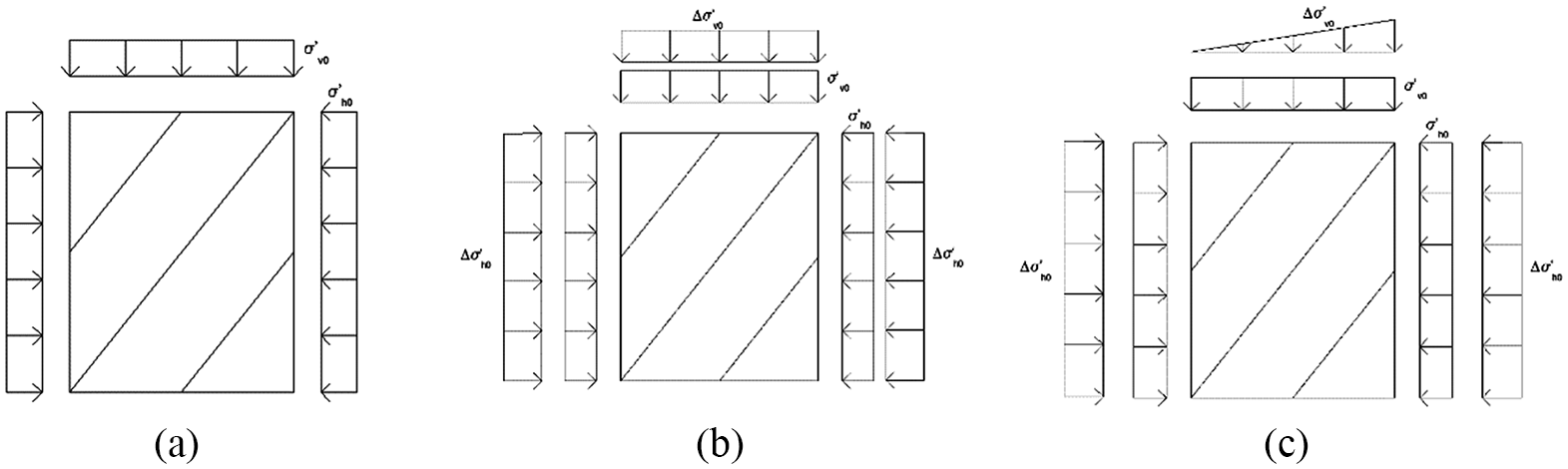
Stress applied to (a) soil element before construction (free field), (b) element A, and (c) element B.

Now, consider the state of stress under free-field conditions for point A and the state of stress at the same element but after construction (A′). When thought of in the classical p′-q plane of critical state soil mechanics, this change in stress can be thought of as passing from point A to point A′, as shown in Figure 3. 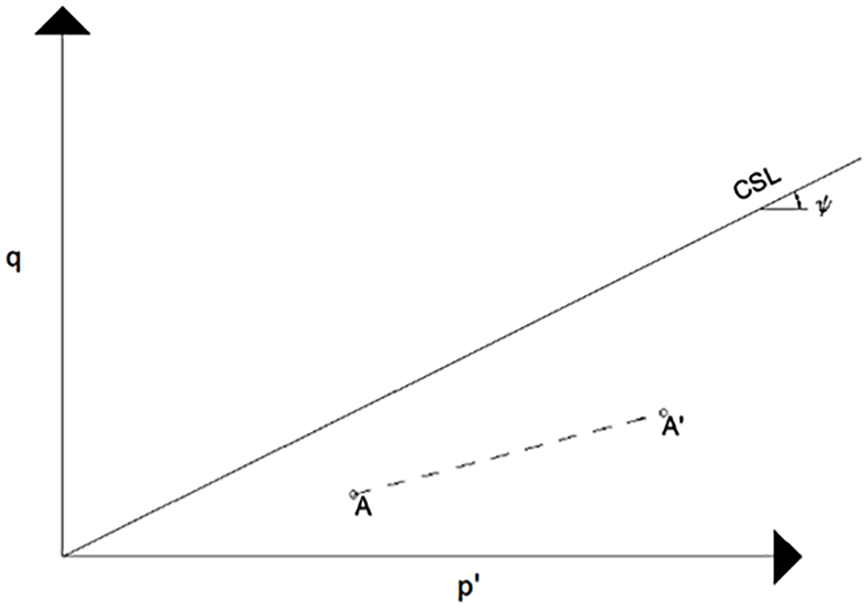The critical state line (CSL) represents an equation giving the magnitude of the deviator stress (q) needed to keep the soil flowing continuously as the product of a frictional constant (M) with effective pressure p ( $q = Mp$ ; Schofield and Wroth, 1968). The angle of the CSL ( $ψ$ ) is directly related to the frictional angle of the Mohr–Coulomb model ( $ϕ$ ) through the relation $\sin (ϕ) = \tan (ψ)$ .

Figure 3.

Evolution of the state of stress for element A—free field to construction (A–A′).

The angle of line AA′ with the spherical axis is given by $α = ta n^{- 1} (Δ q / Δ p')$ , where $Δ q$ and $Δ p'$ relate to the change in spherical and deviatoric stresses between the free-field and constructed conditions. Angle $α$ always yields lower values than angle $ψ$ for choices of $ϕ$ that are smaller than ≈48°. This means that, for element A, since the distance to the CSL will increase with greater confinement from the structural loading, a higher value of deviatoric stress can be applied before reaching the CSL. This also means that the stress path should start at point A′ rather than point A at the kinematic analysis stage. This effect is not considered at the kinematic analysis stage of the substructure methods because structural loads are not considered in the analysis.

For soil element B, the picture is more complicated and depends on the solution to the eigen problem, which will give the rotation of the principal planes and allow for calculation of deviatoric and spherical stresses. At a given depth, this solution will largely depend on the relative position of the element with regard to foundation CSL (Figure 1). Because net increases in stress depend upon both depth and distance to the foundation, direct calculation is cumbersome. However, using a direct approach to the DSSI model, the stress within each element can easily be computed. The problem can thus be managed with the proper selection of element sizes. In any case, the results are the same as for element A, namely, a different initial position for the stress path and a different distance to the CSL.

The cumulative impact of these two shortcomings of the usual substructure approach is that the initial state of stress in the supporting soil element is different than what would be expected under actual loading conditions, resulting in an incorrect initial position on the p′-q plane.

The objective of this article is thus to examine the effect of ISFH in a nonlinear, DSSI finite-element analysis conducted in the time domain using the direct approach in the geo-tectonic context specific to Eastern Canada and evaluate its impact through an application example. The work is presented in two parts.

In part 1, the algorithm developed to analyze ISFH is presented along with its theoretical background. The algorithm was implemented as part of a finite-element program developed in-house using the OpenSees (OS) platform (McKenna et al., 2010).

In part 2, the algorithm developed in part 1 is included in a complete DSSI analysis of a building resting on the same soil deposit to determine the impact of including the effect of ISFH on the dynamic behavior of the structure. The building was a three-story, three-bay reinforced-concrete (RC), moment-resisting structure with masonry infill walls typical of school buildings found in the province of Quebec (Canada) in the 1960s. The dynamic response of the building was analyzed by comparing floor accelerations to relative displacements.

Soil properties were carefully selected based on data from an actual soil deposit that yielded high-quality in situ and laboratory geotechnical and geophysical data (Crow et al., 2017). The site, a deep, sensitive clay deposit in Eastern Canada, was selected for its high potential for DSSI effects. In both parts 1 and 2, the strong ground motion used was compatible with Eastern Canadian earthquakes characterized by a high-frequency content (Atkinson and Boore, 1995).

Methodology

This section covers the selected soil deposit data, the details of the numerical soil model, the stress–strain relationships used, the simulation plan for both parts 1 and 2, and the strong ground motion used for transient loading.

Selected soil deposit

The selected soil deposit is located close to the Quebec–Ontario border, in the Pontiac area called the Breckenridge Valley, which is part of the Champlain’s sea pool (Quigley, 1980). This deep soil deposit is mainly composed of post-glacial marine clay and silt with higher concentrations of sand at depths greater than 63.9 m. Sampling was stopped at this depth due to the artesian conditions present in the region. Geophysical measurements estimated the depth of the soil deposit at 85 m (Hunter et al., 2010). The mean plasticity index (PI) of the collected samples was 37. The exhaustive in situ geotechnical testing, geophysical measurements, and laboratory testing carried out on the selected soil deposit by the Geological Survey of Canada (GSC; Crow et al., 2017) allowed for a clear definition of the site’s geotechnical properties. The water table at the site was estimated to be approximately 5 m deep. The laboratory testing was conducted by the GSC and Duguay-Blanchette (2016). The geotechnical data used in the laboratory tests included unremoulded shear resistance (C_u-fc) and remolded shear resistance (C_r-fc) obtained from the Swedish fall cone test, the Atterberg limits, and the determination of grain size distribution and water content (w). In situ variations in shear wave velocity (V_s), undrained shear resistance ( $C_{u - fc}$ ), and soil mass density (ρ) are shown in Figure 4.

Figure 4.

Geotechnical profile of soil deposit: (a) soil mass density (ρ), (b) $C_{u - fc}$ , and (c) measured shear wave velocity (V_s).

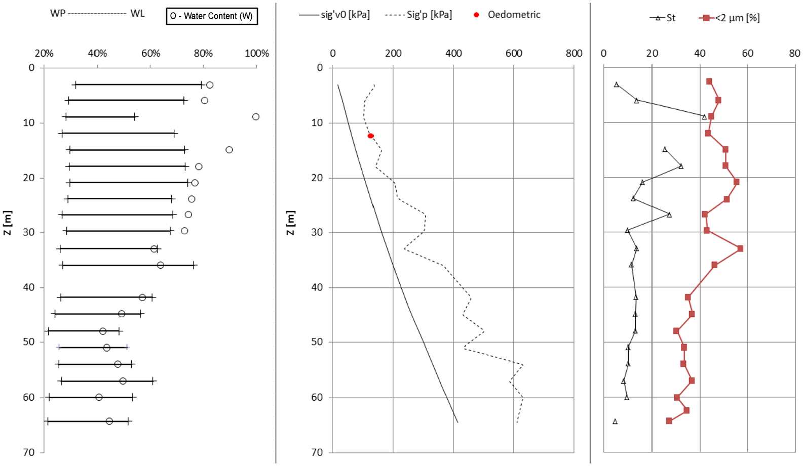
Figure 5 shows the water content (w) and effective ( $σ'_{v 0}$ ) and preconsolidation ( $σ'_{p}$ ) stresses, as well as sensitivity $S_{t}$ and clay fraction ( $< 2 μ m$ ) as a function of depth (z).

Figure 5.

Water content, effective and preconsolidation stress, sensitivity, and percentage of clay as a function of depth (Crow et al., 2017).

Preconsolidation stress and sensitivity values were estimated using the empirical correlation developed for Champlain Sea clay (Leroueil et al., 1983). The result of the oedometer test conducted at depth z = 12.35 m (Duguay-Blanchette, 2016) differed from the empirical calculation of 2.37%. The geophysical measurements of V_s with depth are shown in Figure 4c. The shear wave velocity (V_s) and soil mass density ( $ρ$ ) were used to calculate the variation with depth in the small shear–strain modulus $(G_{\max})$ from Equation 1 (Youn et al., 2008):

G_{\max} = ρ V_{s}^{2}

(1)

The basic geotechnical values used to define the PressureIndependMultiYield (PIMY) material were ρ, $C_{u - fc}$ , V_s (Figure 4), and G_max (Equation 1) with depth. The value of K was easily obtained from the value of G using Equation 2, where v is Poisson’s ratio, used as $v$ = 0.3 in this study:

\frac{2 G (1 + v)}{3 (1 - 2 v)}

(2)

Numerical soil model

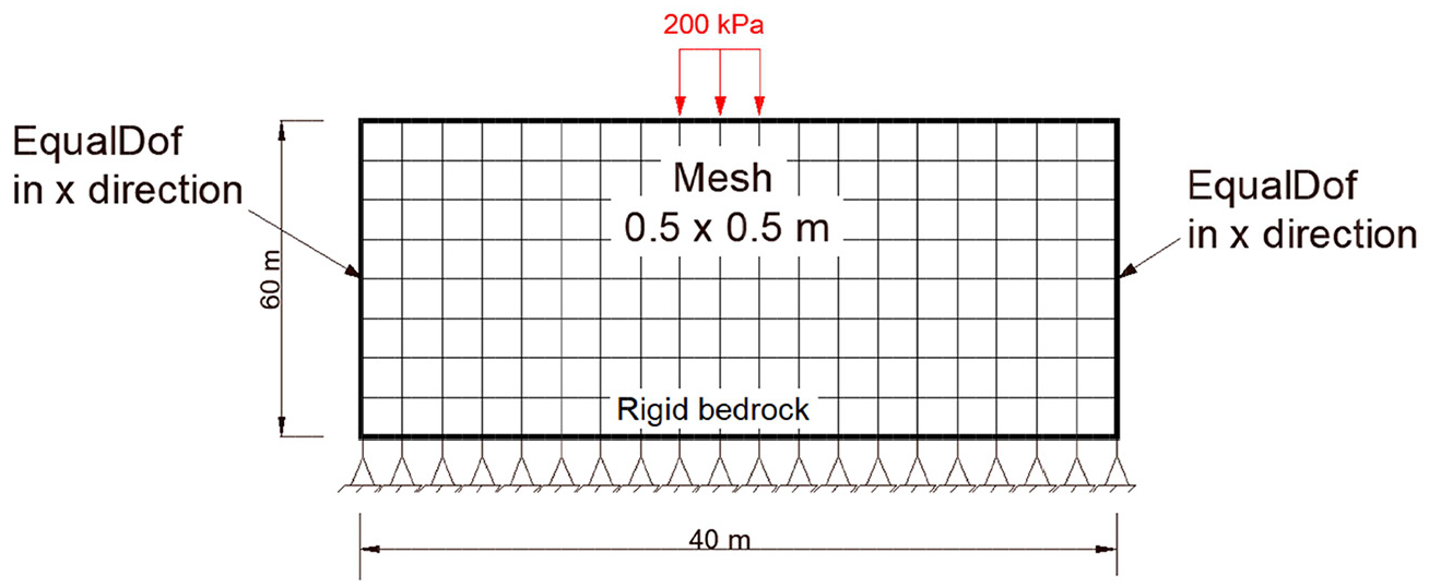
All soil models and numerical simulations were carried out using the OS finite-element platform, which allows for nonlinear dynamic analysis of large numerical systems. Each soil model was built as a two-dimensional (2D) assembly of plane-strain, quadrilateral, stabilized single-point, isoparametric elements (McGann et al., 2012). Mesh dimensions were selected in accordance with the standard conditions for accurate wave propagation of up to 25 Hz (Kuhlemeyer and Lysmer, 1973) ( $\approx λ / 10$ ). The width (W) of the model was established at 40 m to ensure proper stress distribution within depth (Figure 6), while its vertical dimension (i.e. depth of the bedrock) was set at 65 m, which roughly corresponds to the maximum depth of the borehole samples. Numerical lateral artificial boundaries were applied using the tied degrees of freedom approach (TDOF; Zienkiewicz et al., 1989; Figure 6), where equal displacement is applied to equally positioned lateral nodes in their respective DOF.

Figure 6.

Schematic view of coupling relation on numerical lateral frontier.

Lateral confinement was applied using lateral force on each node of the artificial lateral boundary. The values of these loads were determined in the preliminary static analysis stage by attaching highly rigid springs to soil elements. The forces in the springs were recorded and used as values for the load intensity. The bottom boundary was considered fixed in the vertical direction and free in the horizontal direction. In all models, a low level of numerical damping was injected to filter out parasitic noise from the Newmark algorithm by selecting γ = 0.6/β = 0.3025 (Boulanger et al., 1999). This necessary numerical damping is related to the resolution algorithm and should not be confused with other sources of damping, which are naturally present in any dynamic system (e.g. material damping). Because all components of our models were nonlinear, physical source of damping were implicitly considered via their material formulation. Hence, Rayleigh damping, which is commonly used in elastic analysis to account for damping in a general manner, was not necessary.

Constitutive soil model

The nonlinearity of soil was achieved using PIMY (Yang et al., 2003) material, a constitutive stress–strain relationship defined in the OS software. The PIMY material, which is based on the Prevost (1985) multisurface plasticity theory, features a series of nested yield surfaces of increasing dimension based on J2 criteria, which make it possible to consider soil hardening at small strain. The number of yield surfaces can vary from 1 to 40. The backbone curve of the PIMY material is defined piecewise in relation to the number of yield surfaces (Figure 7) and is thus an approximation of the Ramberg– Osgood model (Ramberg and Osgood, 1943). 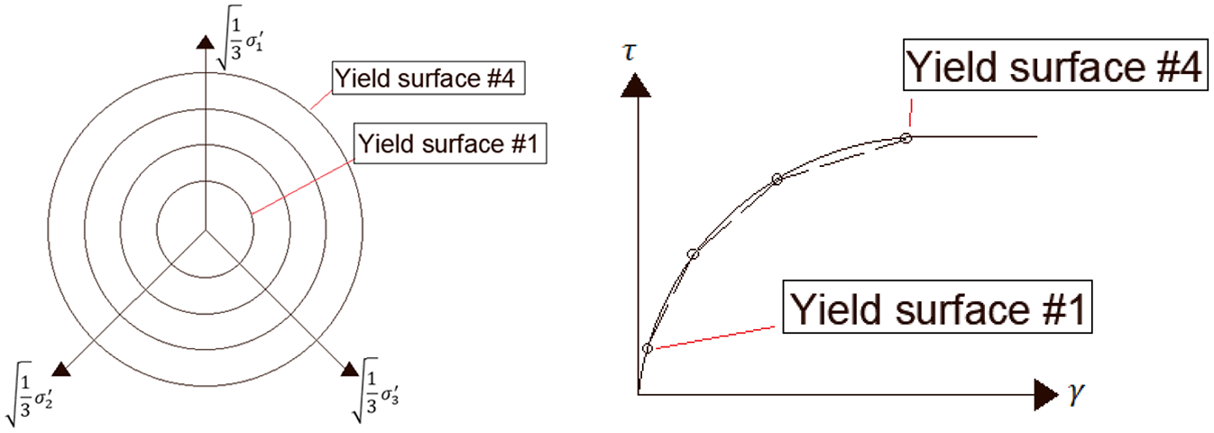Alternatively, the user can define their own backbone curve by providing a series of $τ, γ$ couples. In this study, the automatic backbone curve was used for the soil models with and without ISFH consideration. While a user-defined G/G_max curve would be recommended in a site-specific DSSI analysis, the choice made for this study still made it possible to examine the effect of IFSH on the structural response.

Figure 7.

Nested surface and skeleton curve of the PIMY material.

Simulation plan

The simulation plan was divided into two stages. In the first part, the effect of ISFH was evaluated by comparing the surface acceleration of three numerical inelastic models to a series of calibrated seismic signals specific to Eastern Canada.

In the second part, an example application of the developed procedure was used in a DSSI problem involving a three-story, three-bay structure resting on the soil deposit used in part 1.

Simulation plan—part 1

The calculated surface accelerations were used to produce elastic response spectra (ERS) with 5% damping, which were then used as a basis of comparison between the models. A site-specific updating process described in the section on the impact of modulus values below was then developed to obtain the spatial distribution of moduli G and K under the applied load, as shown in Figure 6.

The results of the PIMY-IND model served as a benchmark for evaluating the impact of soil ISFH. For this model, the iterative process for the G and K moduli was not implemented and standard nonlinear analysis was conducted.

The results of the PIMY-DEP model served to evaluate the impact of the updating procedure itself. In this model, the iterative process was applied while keeping all other aspects similar to those of the PIMY-IND model. The results of the comparative analysis conducted using the ERS calculated from the surface accelerations were then used to assess the impact of the updating process.

In the last model, PIMY-DEP200, the iterative process was implemented with a surface stress of 200 kPa. The surface pressure was applied as vertical load on three distinct nodes, resulting in a footing of width B = 1 m. This surface stress created a net increase in the soil confinement, which dissipated with both depth and width. A comparative analysis was then conducted using the ERS calculated from the surface acceleration obtained with this model. Table 1 provides an overview of the simulation plan.

Table 1.

Parameters of the simulation plan—part 1

Analysis	ISFH	Applied surface stress	Earthquake
Analysis	ISFH	Applied surface stress	M _w 6—D = 30 km	M _w 7—D = 90 km	Historic
PIMY-IND	No	0	M6-1	M7-1	Saguenay 1988 Station St-Ferréol (ENR)
PIMY-IND	No	0	M6-2	M7-2
PIMY-DEP	Yes	0	M6-3	M7-3
PIMY-DEP	Yes	0	M6-4	M7-4
PIMY-DEP200	Yes	200 kPa	M6-5	M7-5

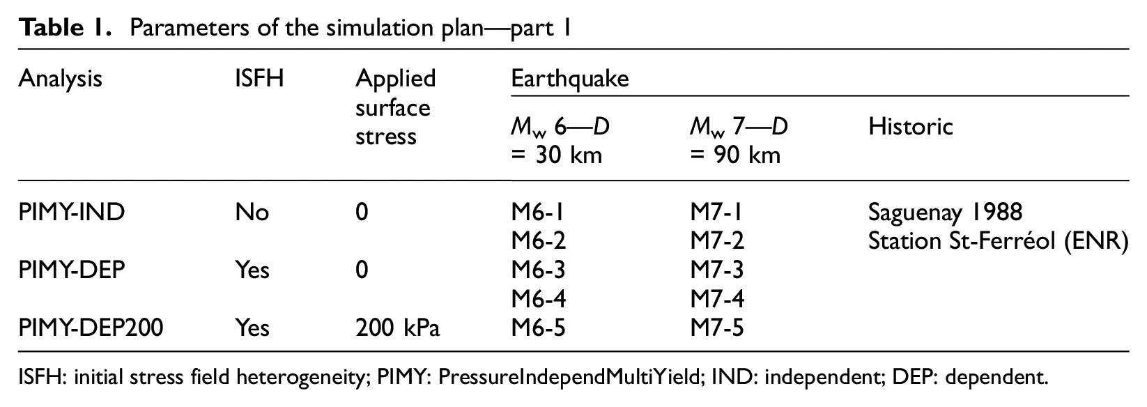
ISFH: initial stress field heterogeneity; PIMY: PressureIndependMultiYield; IND: independent; DEP: dependent.

Simulation plan—part 2

In part 2 of the simulation plan, the impact of ISFH on floor acceleration and relative displacement was examined by analyzing the DSSI effect on a three-story, three-bay structure (Figure 17) resting on the soil deposit described above. The direct approach was used to evaluate the impact of DSSI on the structure. In a first series of analyses (M1), the effect of ISFH was disregarded, while in a second series of analyses (M2) it was considered using the process outlined in the section on the impact of modulus values below. The dynamic input used constituted the complete set of signals described in the following subsection.

Ground motion

The seismic signals used for the dynamic analysis were 10 eastern-specific synthetic signals (Atkinson and Assatourians, 2008) and one historical accelerogram (Mitchell et al., 1989). Each signal was calibrated against the National Building Code of Canada standard NBCC-2015 (National Research Council Canada (NRCC), 2015) design spectrum for rock conditions for a class-A site in Quebec City using the spectral time domain method wavelet algorithm (Abrahamson, 1992). The earthquake magnitude and distance (M-R) considered in the calibration of the seismic signals were scenario 1 for 0.075 ≤ T ≤ 0.5, M-R = 6-30 and scenario 2 for 0.5 ≤ T ≤ 4 M-R = 7-90 (Halchuk et al., 2007). Each dynamic signal was applied at the base of the soil profile, which was considered to be the rigid bedrock. Table 2 provides the peak ground acceleration (PGA) values for each of the 10 calibrated synthetic signals.

Table 2.

PGA of selected synthetic signals

Scenario 1 R = 30 km		Scenario 2 R = 90 km		Historic Saguenay (1988) Station St-Ferréol (ENR)
Signal #	PGA (m/s²)	Signal #	PGA (m/s²)	Signal #	PGA (m/s²)
M6-1	4.15	M7-1	5.88	Saguenay	1.19
M6-2	2.26	M7-2	5.17
M6-3	2.29	M7-3	5.50
M6-4	2.14	M7-4	3.69
M6-5	1.95	M7-5	3.72

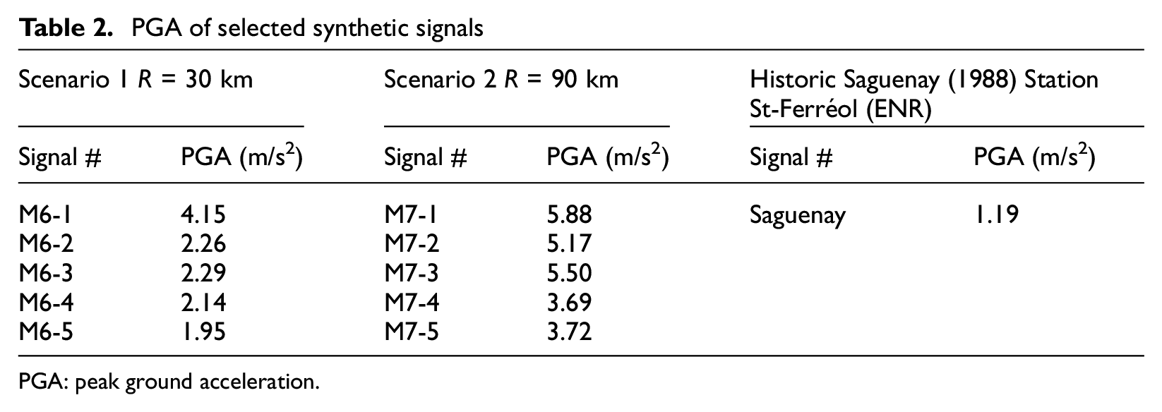
PGA: peak ground acceleration.

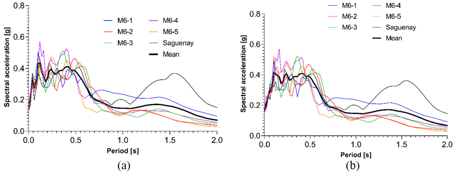
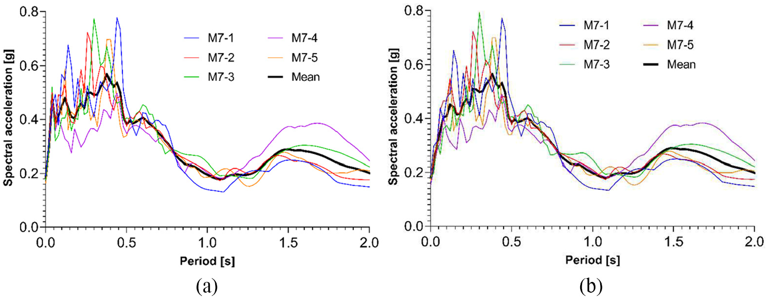
The ERS for the signals calibrated to a maximum of 2 s for scenario 1 are provided in Figure 8a and those for scenario 2 are shown in Figure 8b.

Figure 8.

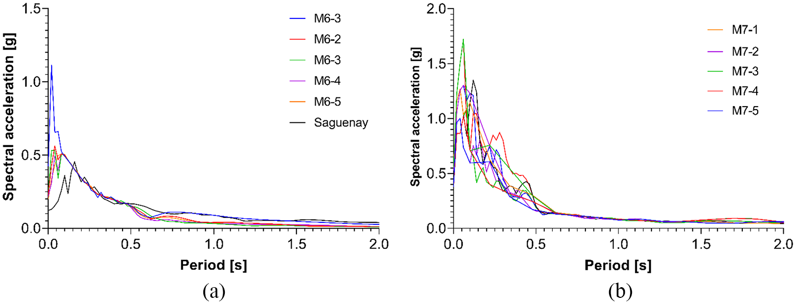
ERS (5%) for calibrated ground motion applied to the base of the model: (a) M_w = 6 and Saguenay (b) M_w = 7.

Modeling of soil stress field heterogeneity

Static initialization of the in situ state of stress

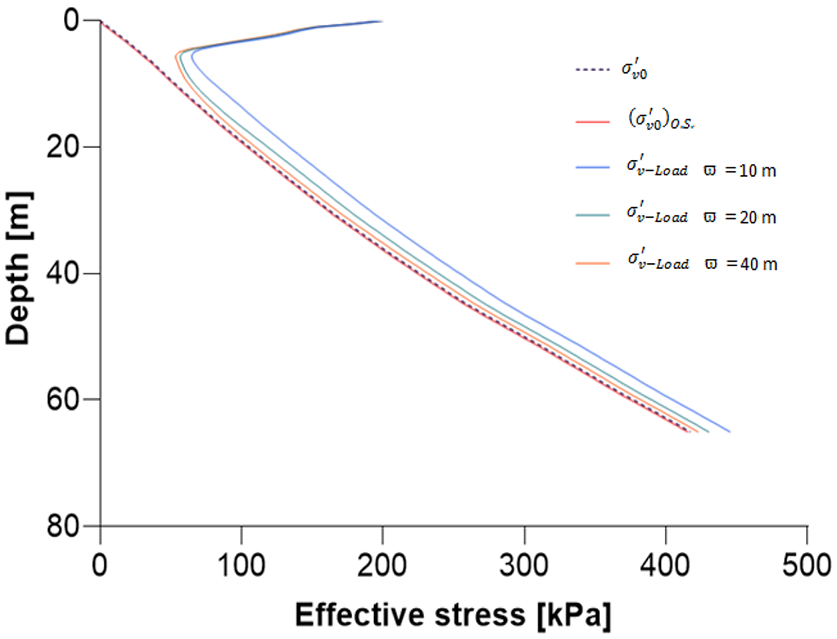
For every numerical model, prior to conducting any dynamic analysis, an initial, static analysis was carried out where the value of the effective stress, $(σ'_{v 0})_{O . S .}$ , was numerically obtained by applying the submerged soil weight density ( $γ' = γ_{total} - γ_{w}$ , where $γ_{total}$ is the saturated soil weight density and $γ_{w}$ is the water weight density) to determine the volumetric forces applied to the finite-element system of equation. Figure 9 shows the variations in the $(σ'_{v 0})_{O . S .}$ values and in the $σ'_{v 0}$ effective stress values obtained from the in situ data as a function of depth.

Figure 9.

Comparison of $(σ'_{v 0})_{O . S .}$ , $σ'_{v 0}$ , and $σ'_{v - Load}$ with depth and of different widths (ϖ) in the numerical soil model.

For model PIMY-DEP200, the state of effective stress under the 200-kPa surface pressure applied at the center of the model ( $σ'_{v - Load}$ ) was calculated. Theoretically, since the net increases in stress from surface pressure should diminish with depth in the soil model, the value of the stress in the soil calculated for model PIMY-DEP200 should approach $σ'_{v 0}$ with increasing depth. However, if the lateral artificial frontier is too narrow, the surface pressure cannot dissipate with depth. It is then important to ensure that the width (ϖ) of the soil model is great enough to correctly propagate the net increases in stress. Figure 9 provides the $σ'_{v - Load}$ value of the numerical model for different widths (ϖ) and with depth. The results show that ϖ = 10 m is the wrong value to use in the numerical soil model and that a ϖ value of at least 40 m is required to correctly propagate the applied 200 kPa surface stress with depth. It should be noted that the difference of 1.4 kPa between the $σ'_{v - Load}$ and $σ'_{v 0}$ values remained constant throughout the depth of the soil model. However, given this relatively small difference and considering that reducing it would imply a wider model and require excessive computational time, the value of ϖ = 40 m was considered acceptable in this case.

Impact of modulus values

This section outlines the procedure followed to calculate the values of the G and K moduli in relation to the value of the effective stress within the element considered. This approach was used for models PIMY-DEP and PIMY-DEP200. In the following sections, we first describe the method and then demonstrate its applicability and its impact in a dynamic analysis.

Estimation of G and K values

Structural loads transferred into the soil result in a heterogeneous increase in the effective stress field in the foundation soil. Previous works have shown that for clay material, there is a dependency of $G_{\max}$ on the value of the effective confinement stress $(σ'_{m} = 1 / 3 (tr (σ))$ , the overconsolidation ratio (OCR) value, and the void ratio ( $e$ ) (Hardin and Black, 1968; Hardin and Drnevich, 1972), which can be expressed as shown in Equation 3 (Vardanega and Bolton, 2013):

G_{\max} = 625 F (e) (OCR)^{k} p_{a}^{1 - n} (σ'_{m})^{n}

(3)

where $p_{a}$ is the atmospheric pressure and $n$ is considered to be 0.5. For this study, OCR values were based on field data (see Figure 5). Different relations have previously been proposed to represent the variations in void ratio with depth F(e) (Hardin, 1978). Consequently, it was possible to calculate the updated initial soil modulus value under the effect of structural loads by implementing a simple algorithm based on Equation 3 in the simulation process.

To do so, the value of $F (e)$ in Equation 3 was obtained by back calculation using Equation 4, where $G_{\max}$ was obtained from Equation 1. A subscript in situ was added to the value of $G_{\max}$ in Equation 4 as it was directly calculated from the field value using Equation 1:

F (e) = \frac{G_{\max - insitu}}{625 {(OCR)}^{k} p_{a}^{1 - n} {(σ_{m}^{'})}^{n}}

(4)

A first static analysis of the numerical model was then run, in which the values of $G_{\max}$ and K were chosen based on the in situ value obtained from Equations 1 and 2. The state of stress within each soil element was then recorded and the value of effective confinement stress $σ'_{m}$ was calculated. A new $G_{\max}$ value, which we refer to as $G_{\max - numerical}$ , was then calculated using Equation 5:

G_{\max - numerical} = 625 F (e) (OCR)^{k} p_{a}^{1 - n} (σ'_{m - numerical})^{n}

(5)

The associated values of K_numerical were then calculated using Equation 2, and the numerical values of $G_{\max - numerical}$ and K_numerical were updated for the element. This process was repeated for each element making up the soil mesh until a stable solution was reached. Because the algorithm was implemented as part of the complete simulation process, the associated stress and strain were preserved for the dynamic analysis.

Difference in modulus as artifact of numerical formulation

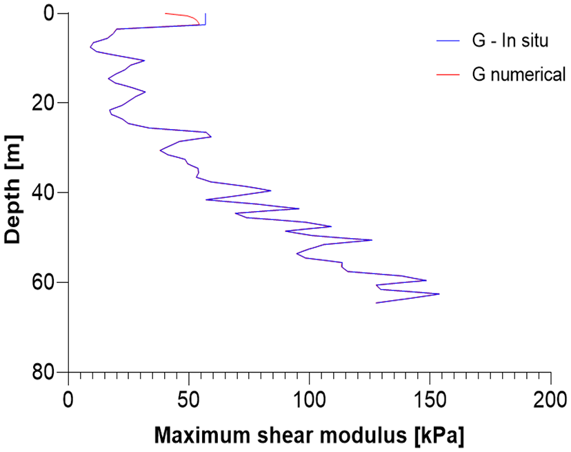
Theoretically, the values of $G_{\max - insitu}$ and $G_{\max - numerical}$ should be identical when no surface pressure is applied to the model, that is, when no net increase in effective stress is present. This was not the case here, however, given the slight difference between the value of $σ'_{m}$ hand-calculated from the in situ data and that calculated in the finite-element model. Figure 10 shows the comparison of $G_{\max - insitu}$ and $G_{\max - numerical}$ with depth following the initial consolidation phase (i.e. without any applied surface loads).

Figure 10.

Comparison of G from in situ value and numerical value with depth.

As can be seen from the results, the numerical and in situ values are relatively similar. The mean difference throughout the depth of the soil deposit for z > 3 m is +0.27% ( $G_{\max - insitu} > G_{\max - numerical}$ ). However, a sudden increase in the difference between the numerical and in situ values can be seen near the surface, with a maximum difference of +29.35% at the surface level. This difference can be explained by considering the numerical and in situ values of the effective confinement stress (see Figure 9). There is a constant difference of ≈1.4 kPa between the numerical and in situ values. This difference, which is insignificant at depth z > 3 m but progressively increases toward the surface, creates a discrepancy between the values of $G_{\max - numerical}$ and $G_{\max - insitu}$ is directly related to the differences in the value of $σ'_{m}$ .

Since the difference between the calculated and numerical value of $σ'_{m}$ was relatively small by comparison to the load transferred from a structure to the supporting soil (1.4 kPa vs 200 kPa), the impact of this difference on the value of $G_{\max - numerical}$ remains insignificant when the load from the structure is applied.

However, in a case where no loading is applied (see model PIMY-DEP in Table 1), it is likely to result in a difference between the dynamic analysis of the soil column using $G_{\max - numerical}$ and that using $G_{\max - insitu}$ . Therefore, to distinguish between the impact of using $G_{\max - numerical}$ and that of increasing the level of effective confining stress, an initial comparative analysis was conducted of the results of the wave-passage calculation obtained with respective soil models using $G_{\max - insitu}$ (Model PIMY-IND) and $G_{\max - numerical}$ (Model PIMY-DEP). The results are provided in the subsection on numerical artifact evaluation in the section on Part 1.

Numerical impact of ISFH

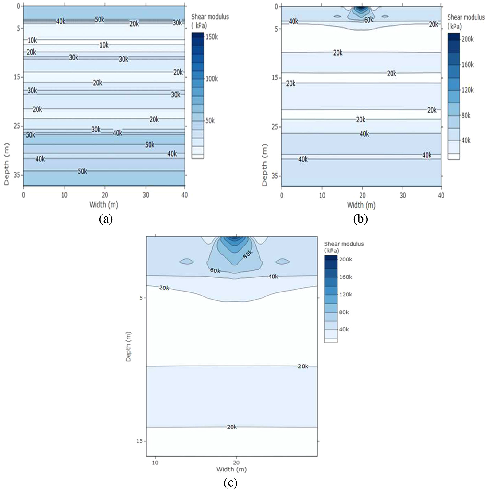
Figure 11a shows the distribution of $G_{\max - numerical}$ with depth for model PIMY-DEP, that is, when no load from the structure is transferred to the supporting soil. Figure 11b shows the distribution of $G_{\max - numerical}$ with depth following the static analysis for model PIMY-DEP200, that is, when a net stress increase of 200 kPa is applied at the surface of the supporting soil. Figure 11c in an enlargement of the impacted zone beneath the applied surface pressure.

Figure 11.

Comparison of impact of ISFH on spatial distribution of moduli values obtained from PIMY-DEP200 analysis: (a) no ISFH, (b) ISFH effect included, and (c) zoom of impacted zone.

As can be seen from the results, the impact of the increase in stress creates a spatial distribution of the value of $G_{\max - numerical}$ that is quite different from the layered distribution shown in Figure 11a. This effect is more pronounced near the surface and gradually decreases to a depth of approximately 5 m. The extent of the influence of the confinement depends on the intensity of the applied load and the dimensions of the footing (B) and can be easily estimated using the Boussinesq relation for stress propagation with depth. The impact of this distribution on a wave-passage analysis is presented in the section covering part 1 below.

Part 1: ISFH analysis results

This section presents the results of the dynamic analysis conducted using the three models described in the “Methodology” section. For each model, the dynamic signals were applied at the base of the soil and surface accelerations were recorded at the surface of the soil deposit. These accelerations were then used to calculate a surface ERS, which served as the basis of comparison between the models.

Results of numerical artifact evaluation

This section provides the results of the evaluation of numerical artifacts used for the above-mentioned ISFH calculation under nonlinear dynamic conditions. Model PIMY-IND, for which no ISFH was calculated, served as the benchmark. Model PIMY-DEP, where ISFH was calculated but no surface load applied, served as the comparative model.

Figure 12a compares the mean ERS value obtained from the surface accelerations calculated using models PIMY-IND and PIMY-DEP for signal M_w 6 and historical earthquake data. Figure 12b compares the mean ERS value obtained from the surface accelerations calculated using models PIMY-IND and PIMY-DEP for signal M_w 7.

Figure 12.

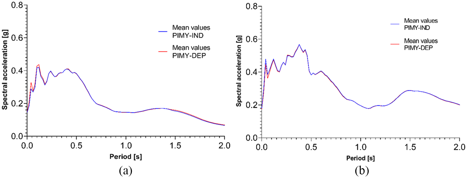
Comparison of the elastic response spectra with 5% damping for M_w 6 earthquake using (a) in situ value and (b) numerical value without surface pressure.

As can be seen, both models produced similar results, which means that the algorithm induced limited error. The greatest differences between the mean values from models PIMY-IND and PIMY-DEP are 0.04 g at T = 0.04 s for M_w 6 and 0.04 g at T = 0.04 s. Therefore, although present, the numerical artifacts remained insignificant and did not significantly alter the dynamic response.

Results of ISFH calculation

This section compares the results of the dynamic analysis conducted using models PIMY-DEP and PIMY-DEP200. In model PIMY-DEP200, ISFH was considered and a pressure of 200 kPa was applied at the soil surface.

The ERS in Figure 13a and b show the respective results from models PIMY-DEP and PIMY-DEP200 for signal M_w 6. There is clearly a difference in amplitude, particularly in the short range (T < 1 s). As expected, the difference in acceleration amplitudes is period-dependent, meaning that the difference between models PIMY-DEP and PIMY-DEP200 is not constant throughout the time period in question but rather varies from period to period. For example, at T = 0.2 s, the difference between the PIMY-DEP200 and PIMY-DEP maximum acceleration values is 0.0357 g (8.87%), while at T = 0.5 s, it is 0.0034 g (0.74%). For some periods, such as T = 0.4 s, the maximum acceleration values from the PIMY-DEP200 model are lower than those from PIMY-DEP (−0.88%).

Figure 13.

Comparison of the elastic response spectra with 5% damping for M_w 6 earthquake using (a) in situ value and (b) numerical value with surface pressure.

Figure 14a and b provide the respective surface acceleration ERS values from models PIMY-DEP and model PIMY-DEP200 for signal M_w 7.

Figure 14.

Comparison of the elastic response spectra with 5% damping for M_w 7 earthquake using (a) in situ value and (b) numerical value with surface pressure.

As was the case for signal M_w 6, the difference in acceleration values between models PIMY-DEP and PIMY-DEP200 is most noticeable for time periods of less than 1 s. The impact of ISFH is very similar for both M_w 7 and M_w 6 signals.

Figure 15a and b shows the mean values from models PIMY-DEP and PIMY-DEP200 for M_w 6 and 7 earthquakes, respectively. As we can see, there are differences in the dynamic responses in the models particularly in the short period range (T < 0.5 s) and in the range of T = 0.7 s.

Figure 15.

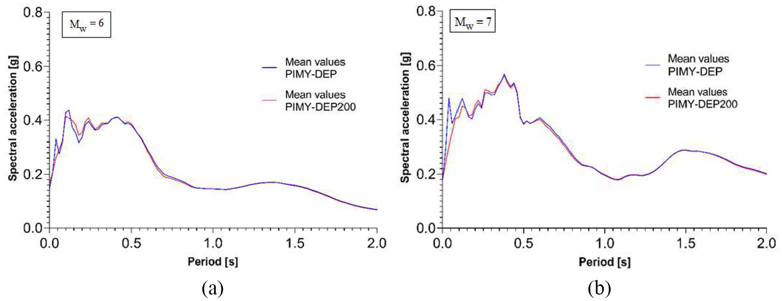
Comparison between mean values in models PIMY-DEP and PIMY-DEP200 for earthquake (a) M_w 6 and (b) M_w 7.

The results show that there was a marked difference in the short range (T < 0.3 s) in both scenarios M_w 6 and M_w 7. Figure 16 provides a clearer picture of the difference between the mean surface acceleration values obtained with models PIMY-DEP and PIMY-DEP200.

Figure 16.

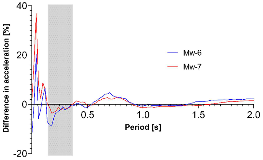
Differences (%) between PIMY-DEP and PIMY-DEP200 for M_w 6 and M_w 7 scenario.

The difference was calculated as follows:

D_{acc} = \frac{PIMY - DE P_{acc} - PIMY - DEP 200_{acc}}{PIMY - DE P_{acc}} .

(6)

When the difference was >0%, the associated PIMY-DEP200 value was lower than that of the PIMY-DEP model. However, when the difference was <0%, the associated PIMY-DEP200 value was higher than that of the PIMY-DEP model. For T < 0.14 s, the PIMY-200DEP model tended to give lower acceleration values than those from the PIMY-DEP model. For 0.14 s < T < 0.36 s (gray zone in Figure 16), the opposite was true and the PIMY-DEP200 values were higher by a mean percentage of 3.6% for scenario M_w 6 and by a percentage of 1.67% for scenario M_w 7. For period range 0.56 s < T < 0.9 s, the PIMY-DEP200 values were lower than those of the PIMY-DEP model by a mean of 2.51% for scenario M_w 6 and by a mean of 1.69% for scenario M_w 7. These results also show that in this case, the relative impact of ISFH was significantly greater for earthquake M_w 6 than for earthquake M_w 7.

To evaluate the impact of soil ISFH, a structure with a seismic resisting force system (SRFS) consisting of a moment-resisting concrete frame with masonry infill walls was considered. The periods of such a structure can be estimated based on Tischer’s (2012) work using Equation 6, where $h_{n}$ is the height of the structure.

T = (0.035 \pm 0.007) {(h_{n})}^{3 / 4}

(7)

The height of a typical three-story institutional building can be estimated at 12 to 15 m (Mestar, 2014). The associated periods would then fall within the range of 0.15 s ≤ T ≤ 0.32 s. For this range of periods and the soil deposit considered, the results show that failure to consider the confinement and anisotropy effect in the dynamic analysis would have caused the acceleration to be underestimated by 7.7% and 1.6%, with a mean value of 4% for earthquake scenario M_w 6. Interestingly, for earthquake scenario M_w 7, the results show that underestimation of the acceleration would be between 0.47% and 1.7%, with a mean value of 1.1%. It can thus be seen that the under- or overestimation of the effect of confinement and stress anisotropy in the soil is not simply a function of earthquake intensity but rather is due to a complex interweaving of signal frequency content and soil properties.

Part 2: application to an existing RC building

The above-mentioned updating procedure used in the ISFH analysis was applied to the study of the DSSI effect on a three-story, three-bay structure resting on the soil deposit described earlier. The direct approach was used to evaluate the impact of ISFH on the structure’s response. ISFH was disregarded in a first series of analyses (M1), but considered in a second series (M2). The dynamic signals used were the same as those previously described in the section covering wave-passage analysis in part 1.

Figure 13 shows the plan view and typical elevation of the hypothetical building studied. This three-story building is typical of the institutional structures built in the province of Quebec in the 1960s. The building was designed in accordance with the provisions of standard NBCC-1965. Further details regarding the design of the building can be found in Apari Lauzier (2016). Lateral loads are resisted by three RC frames in the long direction and four frames in the short direction. This example focuses on one of the three-bay interior frames in the short direction (circled in red in Figure 17). The RC frame is erected on four separate surface footings located 2 m below ground level for frost protection. Eigen analysis yielded a fundamental period of 0.66 s for the soil–structure multi-DOF (MDOF) system, while Equation 6 gave an estimate of 0.54 s. The difference is attributable to the fact that Equation 6 did not consider the foundation soil type as it was derived from ambient vibrations from structures on more competent soil than that considered in this work. Consequently, the value of 0.66 s was used as the structure’s fundamental period. For this period, according to Figure 16, we should expect a decrease in prescribed structural accelerations at the RC level in the range of 5% to 6 % for a scenario 1 earthquake (blue line), whereas a scenario 2 earthquake (red line) would also show a decrease in accelerations on the order of 4%. It is important to note that this assumption is based on the idea that the structure will remain in the elastic range. When structural elements yield, the solution to the eigen problem changes because of a reduction in structural rigidity, which, in turn, results in period elongation. Hence, depending on the level of yield in the structural elements, the expected value in Figure 16 will vary.

Figure 17.

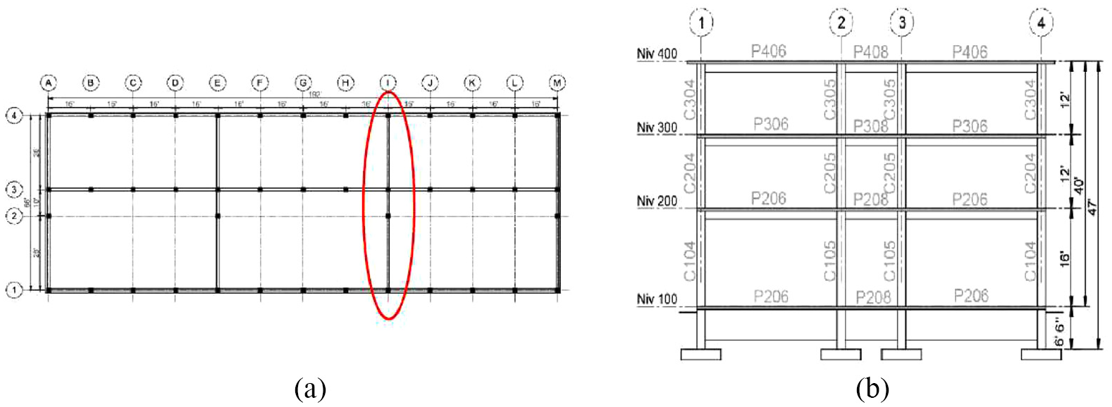
(a) Floor plan (Apari and Lauzier, 2016) and (b) elevation view of building studied.

The calculated data include displacements and accelerations at each story of the structure. Story displacements were subtracted from basement displacements to yield relative displacement, which were used for comparison purposes. Acceleration values were reported as either positive or negative, indicating the direction of the acceleration. A negative value indicates that the acceleration was directed toward the left (Figure 17b), while a positive value indicates the acceleration was directed to the right.

Numerical model

The numerical model for the frame structure was built using nonlinear BeamColumn elements available in the OS element library. Each section was discretized into fibers for which the nonlinear material stress–strain response was defined. Distinct fibers were defined for confined and unconfined concrete zones and for the steel reinforcement. The fiber section model considered the bending moment and axial load interaction, but the shear–bending or shear–axial load interactions could not be represented. To represent concrete inelastic behavior, the uniaxial Kent–Scott–Park model with linear tension softening (Concrete02; Mohd Yassin, 1994) was applied. The Giuffré–Menegotto–Pinto (Steel02; Filippou et al., 1983) hysteretic material was employed to describe the inelastic behavior of the reinforcing bars. Specific values used in the definition of the steel and concrete model can readily be found in Apari Lauzier et al. (2017). The nonlinear solution for the BeamColumn elements was based on the iterative force procedure using the Gauss–Lobatto integration point. To ensure a proper local solution, a total of seven integration points were selected on each member in accordance with the recommendations found in the literature Neuenhofer and Filippou (1997).

To model the soil–structure interface, the node making up the footing and the corresponding node constituting the soil element were directly linked using a coupling relation. The nodes used in the soil domain had two DOFs, while the nodes in the structural model had three. An additional series of nodes, referred to as ghost nodes, was inserted at the soil–structure interface. The ghost nodes had no physical meaning; they merely served as a numerical bridge. The ghost nodes were defined in the structural domain as having three DOFs, the third being fixed, that is, having zero rotation. The soil node displacements along two DOFs were expected to coincide with the two ghost translational DOFs. The ghost nodes were then linked to the structural nodes at the base of the footing using the zeroLength element, to which specific uniaxial material properties can be assigned, irrespective of the direction considered. This approach allows for defining various horizontal, vertical, and rotational contact conditions. For this study, a “glue”-type link was used at the soil–structure interface to prevent the footing from slipping or lifting. The seismic signal was then applied at the base of the soil model, resulting in immediate transfer of the excitation to the structure. In this series of analyses, the soil model extended 190 m from the structure in either direction to minimize lateral frontier impact. The rest of the numerical soil model was similar to that used for the wave-passage analysis described earlier.

Structural response to transient loading

Acceleration

Figure 18a provides the comparative results of scenario 1 signal M6-2 floor accelerations for model M1, where ISFH was ignored and model M2, where ISFH was considered. Figure 18b shows the mean floor acceleration values for scenario 1, models M1 and M2.

Figure 18.

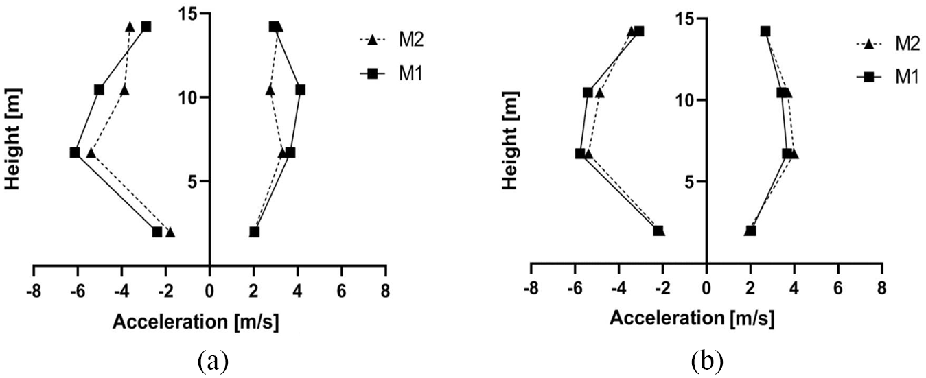
Comparison of acceleration values (minimum and maximum) in models M1 (effect of ISFH disregarded) and M2 (effect of ISFH considered) for (a) scenario 1 signal M6-2 and (b) mean values for all signals in scenario 1.

For signal M6-2 in scenario 1, ISFH yielded a mean decrease in acceleration of 14.02% for the entire structure. However, the results obtained for each story are more complex. At the roof level, ISFH yielded an increase in acceleration of up to 20%. At the main-floor level, the acceleration values calculated for the first and second stories using model M2 were higher by a mean value of 23%. Considering all scenario 1 signals (Figure 18b), the results indicate that ISFH yielded a decrease in maximum acceleration values of 0.44%. Here again, there was significant variation in the values for each story. ISFH increased the mean acceleration values at the roof level and the first two stories by 4.77% and 0.42%, respectively. However, at the second-story and main-floor levels, it decreased acceleration by 1.73% and 5.24%, respectively. These values are in line with those shown in Figure 16 (blue line) and suggest limited yielding in the structural elements.

Figure 19a shows the moment–axial interaction load curve (M–P) of the external columns (axes 1 and 4 in Figure 17b) for earthquake signal M6-2. As can be seen, little or no yielding occurred for this signal. The same situation was observed in all other loading scenarios with the exception of signal M6-1, where yielding did occur. Figure 18 illustrates the hypothesis of a fixed-period hold for scenario 1 signals, which correlate with calculated accelerations at the main-floor level.

Figure 19.

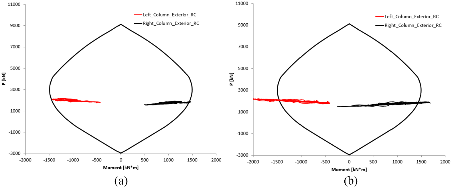
M–P interaction curve for exterior RC columns for (a) scenario 1 signal M6-2 and (b) scenario 2 signals M7-3 and M2 (effect of ISFH considered) and for (a) scenario 1 signal M6-2 and (b) mean values for all signals in scenario 1.

The results for scenario 2 show a mean decrease in main-floor accelerations of 0.58%, while Figure 16 shows an anticipated decrease on the order of 4%. This can easily be explained by the yielding observed in several elements of the structure for all signals in scenario 2. Figure 19b shows the M–P interaction load curve for the external columns (axes 1 and 4 in Figure 17b) for earthquake signal M7-3. The results clearly show that there was yielding in the column during loading, which led to period elongation on the order of 36% during peak earthquake loading. This explains there was less reduction in acceleration values for this scenario. Similar results were obtained for all signals in scenario 2.

The results thus demonstrate that taking ISFH into consideration had a major impact on the acceleration values calculated for the structure. As expected, the results also show that the impact of ISFH depends on the nature of the dynamic signal (i.e. intensity and frequency content), type of soil deposit, and structural characteristic of the building.

Structural displacement relative to foundation

Figure 20a shows the relative displacement values for scenario 1 signal M6-2 from models M1 (ISFH ignored) and M2 (ISFH considered). Figure 20b shows the mean relative displacement values for the scenario 1 signals from models M1 and M2. Figure 21a and b, respectively, provides the relative displacement values for scenario 2 signal M7-4 and the mean relative displacement values for the entire set of signals in scenario 2.

Figure 20.

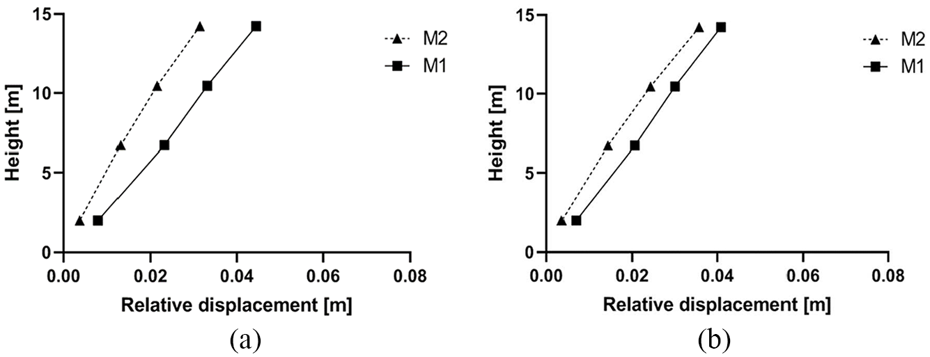
Comparison of relative displacement values from models M1 (effect of ISFH disregarded) and M2 (effect of ISFH considered) for (a) scenario 1 signal M6-2 and (b) mean value of all signals in scenario 1.

Figure 21.

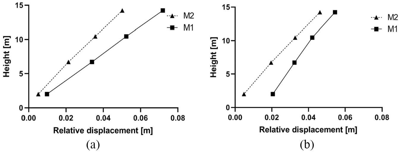
Comparison of relative displacement in models M1 (effect of ISFH disregarded) and M2 (effect of ISFH considered) for (a) scenario 2 signal M7-4 and (b) mean values for all signals in scenario 2.

The results for scenario 1 signal M6-2 show that the consideration of ISFH decreased relative displacement by a mean value of 40%. This general downward trend was observed on every story and for every signal. Consequently, the mean relative displacement values for scenario 1 decreased by 27.7% when ISFH was considered, which is consistent with the expected results shown in Figure 16.

As can be seen in Figure 21, a similar decrease in relative displacement was observed for the signals in scenario 2. Signal M7-4 in scenario 2 yielded a mean decrease in relative displacement of 36.8%. A similar trend was observed for all signals. The mean decrease in relative displacement for all signals in scenario 2 was 38.4%. The yielding observed in the column during the scenario 2 signals explains the apparently significant reduction in relative displacement, considering the small decrease in acceleration.

The fact that ISFH caused a decrease in relative displacement is not surprising, considering that it increased the supporting soil moduli values. The downward trend was observed for all signals, irrespective of the intensity or frequency content considered.

Conclusion

The objective of this article was to investigate the effect of ISFH in a nonlinear DSSI numerical finite-element analysis conducted in the time domain using the direct approach for the geotechnical and seismological context specific to Eastern Canada, and to evaluate its impact through an application example.

In part 1, a numerical algorithm was developed to consider ISFH. A series of wave-passage analyses was carried out to assess the impact of ISFH on the dynamic response of a natural soil deposit located in Eastern Canada. In this part, a surface load was applied to the soil model and the impact of ISFH was either considered or ignored.

In part 2, the algorithm developed in Part 1 was included in the comprehensive DSSI analysis of a building resting on the same soil deposit to determine the impact of considering ISFH on the dynamic behavior of the structure. The building considered was a three-story, three-bay RC moment-resisting structure with masonry infill walls typical of the institutional buildings found in the province of Quebec in the 1960s. Two distinct sets of DSSI analyses were conducted where stress field heterogeneity was either considered or not.

The results from part 1 reveal that the net increase in the soil’s effective stress from the applied surface pressure caused an increase in the shear and bulk moduli in the supporting soil of the structure, thus creating a bulb-like zone beneath the footing with a higher rigidity than under natural conditions (i.e. with no structure). The results of the subsequent wave-passage analysis show that the impact of this increased-rigidity zone beneath the foundation led to a modification of the calculated surface acceleration values, which varied depending on the periods considered. For example, for period T < 0.14, consideration of ISFH in the supporting soil resulted in a decrease in calculated surface accelerations. However, in period range 0.14 < T < 0.36, the opposite happened, and the calculated surface accelerations increased by mean values of 3.6% for a scenario 1 earthquake and 1.67% for a scenario 2 earthquake. Interestingly, the results seem to indicate that the impact of considering ISFH on calculated surface accelerations was not related to the intensity of the shaking but rather, to signal frequency content versus soil deposit rigidity. Hence, the results suggest that for a structure with fundamental periods (T) of 0.15–0.32 s, soil ISFH would tend to increase mean surface acceleration values by 4% in the case of signal M_w 6 and by up to 1.1% for signal M_w 7. In this case, the maximum increase in calculated surface acceleration values was 7.7%. Conversely, for a different period interval, prescribed surface accelerations would decrease, as demonstrated in part 2 of the study. While the effect of ISFH is relatively minor (i.e. a difference in surface accelerations of less than 8% in this case), the difference may be greater in buildings supported on mat foundations with high bearing stress, as a larger zone of soil would be affected. On the contrary, ignoring IFSH would probably not have a significant effect on surface accelerations in pile-supported structures as there would be minimal transfer of structure stress to the ground, although further studies should be conducted to demonstrate this.

The results of part 2 reveal that for an MDOF soil–structure system with periods of around 0.66 s, the effect of ISFH was to reduce prescribed mean structural accelerations and displacement at the main-floor level in the range of ≈5% for a scenario 1 earthquake and ≈0.6% for a scenario 2 earthquake. These results are in line with the findings of the wave-passage analysis, which demonstrated that, for this range of periods, taking ISFH into account would lead to a decrease in structural accelerations applied at the base of the structure. This finding has major implications as failure to consider the effect of ISFH may lead to miscalculations in prescribed structural accelerations, that is, over- or underestimation of the magnitude of the acceleration. This phenomenon is complex as it is directly related to the frequency content of the applied signal, the geotechnical properties of the soil deposit and the structural characteristics of the building considered. Considering that it is relatively simple to take ISFH into consideration in the calculation and given its potential impact on the result, this natural soil characteristic should be considered in all DSSI analyses.

The results of this study are based on a single soil deposit and a limited number of signals. Further work is needed to increase the variability of the dynamic signal used, and the characteristics of the soil models (i.e. investigate different types of soil deposit) and structures.

It is worth noting that the ISFH calculation procedure described in this article considers the void ratio to be constant. This assumption is wrong in the case of the initial stress application as the soil is expected to be loaded for several years, that is, in drained conditions, prior to experiencing an earthquake. In the context of critical state soil mechanics, this problem involves a relationship between deviatoric stress, volumetric effective stress, and void ratio; work is ongoing to consider this aspect of the problem.

Footnotes

Acknowledgements

We acknowledge the support of the Fonds de Recherche Nature et Technologie du Québec.

Declaration of conflicting interests

The author(s) declared no potential conflicts of interest with respect to the research, authorship, and/or publication of this article.

Funding

The author(s) received no financial support for the research, authorship, and/or publication of this article.

ORCID iDs

Marc-Denis Rioux

Bertrand Galy

References

Abrahamson

(1992) Non-stationary spectral matching. Seismological Research Letters 63: 30.

Apari Lauzier

J-S

(2016) L’impact de l’interaction Sol-structure Sur l’évaluation Sismique des Cadres Rigides en Béton Armé Existants Situés dans l’est du Canada. Master’s Thesis, École Polytechnique de Montréal, Montréal, QC, Canada.

Apari Lauzier

J-S

Koboevic

Nollet

(2017) Impact of soil-structure interaction effects on seismic assessment in moderate seismic zones. Paper presented at the 16th world conference on earthquake engineering, Santiago, 9–13 January.

Atkinson

Assatourians

(2008) Engineering seismology toolbox. Available at: https://www.seismotoolbox.ca/ (accessed on April 2018)

Atkinson

Boore

(1995) Ground-motion relations for eastern North America. Bulletin of the Seismological Society of America 85: 17–30.

Avilès

Pérez-Rocha

(1998) Site effects and soil-structure interaction in the valley of Mexico. Soil Dynamics and Earthquake Engineering 17: 29–39.

Boulanger

Curras

Kutter

Wilson

Abghari

(1999) Seismic soil-pile-structure interaction experiments and analyses. Journal of Geotechnical and Geoenvironmental Engineering 125: 750–759.

Boussinesq

(1885) Application des potentiels à l’étude de l’équilibre et du mouvement des solides élastiques, principalement au calcul des deformations et des pressions que produisent, dans ces solides, des efforts quelconques exercés sur und petite partie de leur surface ou de leur intérieur; memoire suivi de notes étendues sur divers points de physique mathématique et d’analyse; par M. J. Boussinesq. Paris: Gauthier-Villars.

Crow

Alpay

Hinton

Knight

Oldenborger

Percival

Pugin

AJM

Pelchat

(2017) Geophysical, Geotechnical, Geochemical, and Mineralogical Data Sets Collected in Champlain Sea Sediments in the Municipality of Pontiac, Quebec (open file 7881). Ottawa, ON, Canada: Natural Resources Canada.

10.

Cubrinovski

Bradley

Wotherspoon

Green

Bray

Wood

Pender

Allen

Bradshaw

Rix

Taylor

Robinson

Henderson

Giorgini

Winkley

Zupan

O’Rourke

DePascale

Wells

(2011) Geotechnical aspects of the 22 February 2011 Christchurch earthquake. Bulletin of the New Zealand Society of Earthquake Engineering 44: 205–226.

11.

Duguay-Blanchette

(2016) Étude du comportement statique et cyclique de deux argiles sensibles de l’Est du Canada. Québec, QC, Canada: Département de Génie Civil, Université Laval.

12.

Filippou

Popov

Bertero

(1983) Effects of bond deterioration on hysteretic behavior of reinforced concrete joints. Report no. UCB/EERC 83-19, August 1983. Berkeley, CA: Earthquake Engineering Research Center, University of California, Berkeley.

13.

Gajan

Kutter

(2008) Capacity, settlement, and energy dissipation of shallow footings subjected to rocking. Journal of Geotechnical and Geoenvironmental Engineering 134: 1129–1141.

14.

Halchuk

Adams

Anglin

(2007) Revised deaggregation of seismic hazard for selected Canadian cities. Paper presented at the 9th Canadian conference on earthquake engineering, Ottawa, ON, Canada, 26–29 June.

15.

Hardin

(1978) The nature of stress-strain behavior for soils. Paper presented at the earthquake engineering and soil dynamics: Proceedings of the ASCE geotechnical engineering division specialty conference, Pasadena, CA, 19–21 June.

16.

Hardin

Black

(1968) Vibration modulus of normally consolidated clay. Journal of the Soil Mechanics and Foundations Division 94: 353–369.

17.

Hardin

Drnevich

(1972) Shear modulus and damping in soils: Design equations and curves. Journal of the Soil Mechanics and Foundations Division 98: 667–692.

18.

Hunter

Crow

Brooks

Pyne

Motazedian

Lamontagne

Pugin

AJM

Pullan

Cartwright

Douma

Burns

Good

Kaheshi-Banab

Caron

Kolaj

Folahan

Dixon

Dion

Duxbury

Landriault

Ter-Emmanuil

Jones

Plastow

Muir

(2010) Seismic Site Classification and Site Period Mapping in the Ottawa Area Using Geophysical Methods. Ottawa, ON, Canada: Geological Survey of Canada.

19.

Jâky

(1944) A nyugalmi nyomâs tényezöje [The coefficient of earth pressure at rest]. Magyar Mérnok és Epitész Egylet Közlönye [Journal for Society of Hungarian Architects and Engineers] 78: 355–358.

20.

Kausel

Whitman

Morray

Elsabee

(1978) The spring method for embedded foundations. Nuclear Engineering and Design 48: 377–392.

21.

Kuhlemeyer

Lysmer

(1973) Finite element method accuracy for wave propagation problems. Journal of the Soil Mechanics and Foundations Division 99: 421–427.

22.

Leroueil

Tavenas

Le Bihan

J-P

(1983) Propriétés caractéristiques des argiles de l’est du Canada. Canadian Geotechnical Journal 20: 681–705.

23.

Lysmer

Udaka

Tsai

Seed

(1975) FLUSH—A Computer Program for Approximate 3-D Analysis of Soil-Structure Interaction Problems. Berkeley, CA: University of California, Berkeley.

24.

McGann

Arduino

Mackenzie-Helnwein

(2012) Stabilized single-point 4-node quadrilateral element for dynamic analysis of fluid saturated porous media. Acta Geotechnica 7: 297–311.

25.

McKenna

Scott

Fenves

(2010) Nonlinear finite-element analysis software architecture using object composition. Journal of Computing in Civil Engineering 24(1): 95–107.

26.

Mestar

(2014) Procédure multi-niveaux pour l’évaluation de la vulnérabilité sismique des écoles dans l’est canadien. Montréal, QC, Canada: Département de Génie De La Construction, École de Technologie Supérieure.

27.

Mitchell

Adams

DeVall

Weichert

(1986) Lessons from the 1985 Mexican earthquake. Canadian Journal of Civil Engineering 13: 535–557.

28.

Mitchell

Tinawi

Law

(1989) Damage caused by the November 25, 1988, Saguenay earthquake. Canadian Journal of Civil Engineering 17: 338–365.

29.

Mohd Yassin

(1994) Nonlinear Analysis of Prestressed Concrete Structures under Monotonic and Cyclic Loads. Berkeley, CA: University of California, Berkeley.

30.

National Research Council Canada (NRCC) (2015) National Building Code of Canada. Ottawa, ON, Canada: NRCC.

31.

Neuenhofer

Filippou

(1997) Evaluation of nonlinear frame finite-element models. Journal of Structural Engineering: ASCE 123: 958–966.

32.

Prevost

(1985) A simple plasticity theory for frictional cohesionless soils. International Journal of Soil Dynamics and Earthquake Engineering 4: 9–17.

33.

Quigley

(1980) Geology, mineralogy, and geochemistry of Canadian soft soils: A geotechnical perspective. Canadian Geotechnical Journal 17: 261–285.

34.

Ramberg

Osgood

(1943) Description of stress-strain curves by three parameters. Report no. NACA-TN-902, 1 July. Washington, DC: National Advisory Committee for Aeronautics.

35.

Reid

(1906) The influence of the foundation on the apparent intensity. In: Reid

(ed.) The California Earthquake of April 18, 1906, vol. 2. Trenton, NJ: State Investigation Commission, p. 49a.

36.

Rogers

(1906) Experiments with a shaking machine. In: Reid

(ed.) The California Earthquake of April 18, 1906, vol. 2. Trenton, NJ: State Investigation Commission, p. 326.

37.

Schofield

Wroth

(1968) Critical State Soil Mechanics. New York: McGraw Hill.

38.

Stewart

Crouse

Hutchinson

Lizundia

Naeim

Ostadan

(2012) Soil-Structure Interaction for Building Structures (NEHRP consultants joint venture). Gaithersburg, MD: National Institute of Standards and Technology.

39.

Stewart

Seed

Fenves

(1999) Seismic soil-structure interaction in buildings. II: Empirical findings. Journal of Geotechnical and Geoenvironmental Engineering 125: 38–48.

40.

Tischer

(2012) Rapid Seismic Vulnerability Assessment of School Buildings in Quebec. Montreal, QC, Canada: McGill University, 234 pp.

41.

Vardanega

Bolton

(2013) Stiffness of clays and silts: Normalizing shear modulus and shear strain. Journal of Geotechnical and Geoenvironmental Engineering 139: 1575–1589.

42.

Yang

Elgamal

Parra

(2003) Computational model for cyclic mobility and associated shear deformation. Journal of Geotechnical and Geoenvironmental Engineering 129: 1119–1127.

43.

Youn

Choo

Kim

(2008) Measurement of small-strain shear modulus G_max of dry and saturated sands by bender element, resonant column, and torsional shear tests. Canadian Geotechnical Journal 45: 1426–1438.

44.

Zienkiewicz

Bicanic

Shen

(1989) Earthquake input definition and the transmitting boundary conditions. In: Doltsinis

(ed.) Advances in Computational Nonlinear Mechanics. Vienna: Springer, pp. 109–138.

Impact of initial stress field heterogeneity in dynamic soil–structure interaction

Abstract

Keywords

Introduction

Methodology

Selected soil deposit

Numerical soil model

Constitutive soil model

Simulation plan

Simulation plan—part 1

Simulation plan—part 2

Ground motion

Modeling of soil stress field heterogeneity

Static initialization of the in situ state of stress

Impact of modulus values

Estimation of G and K values

Difference in modulus as artifact of numerical formulation

Numerical impact of ISFH

Part 1: ISFH analysis results

Results of numerical artifact evaluation

Results of ISFH calculation

Part 2: application to an existing RC building

Numerical model

Structural response to transient loading

Acceleration

Structural displacement relative to foundation

Conclusion

Footnotes

Acknowledgements

Declaration of conflicting interests

Funding

ORCID iDs

References