Classification and Peroxide Value Prediction of Naturally Aged Edible Oils Using Raman and Infrared Spectral Analysis

Abstract

Developing global classification and calibration models for identifying edible oil type and predicting peroxide value, a measure of the degree of oxidation directly related to oil freshness is predicated on capturing variance differences within and between growing seasons across a large set of 19 naturally aged (5–7 years) oil types. Our approach utilizes a larger sample set and longer aging period than reported studies (typically 2–5 years), includes multiple growing seasons, and is based on natural rather than accelerated thermal aging of oil samples. We provide spectroscopic data (Raman scattering, near- and mid-infrared absorption) for 19 edible oil types, which represent the most diverse and only naturally aged sample set reported to date. The data, which consist of three data collection campaigns acquired using different analytical methods at different times during the aging process, provide opportunities to investigate and validate new machine learning approaches for classification, calibration, and data fusion. In the supplemental material, vibrational spectroscopy data from all samples are included along with the R programming language code for preprocessing data and building basic classification and calibration models.

Graphical abstract

This is a visual representation of the abstract.

Introduction

Motivation

Chemometrics and machine learning techniques play an increasingly essential role in the spectroscopy data analysis pipeline of complex, dynamic chemical processes. Thus, optimally extracting information from multivariate spectroscopic signals, gathered during observations of a multivariate chemical process, requires multivariate statistical methods. A recent workshop, “Envisioning Data Driven Advances in Measurement and Instrumentation for Chemical Discovery", noted in the recommendations that to maintain a healthy ecosystem of chemical measurement science, chemical data science needs to foster learning opportunities in chemometrics among measurement scientists and provide well curated and widely accessible multivariate data sets for method development, benchmarking, and educational opportunities. This investigation strives to meet both of these workshop recommendations. First, we present a collection of real-world vibrational spectroscopy data for classification of edible oils by plant origin and calibration to determine freshness as defined by the oil peroxide value (PV). Such data are envisioned to be useful for testing and comparing new chemometric algorithms for model development, baseline removal, and variable selection. Second, we present the data through a tutorial by building basic classification and calibration models in the R programming environment. While many vendors sell excellent dashboards or toolboxes for guided development of chemometric analyses, commercial software is not universally available to all students or professionals seeking to independently expand their skill base. R, a statistical programming language, such as the closely related Python programming language, is an open-access environment with many free libraries of code (i.e., packages) available that are designed for the development of classification and calibration models.

Background

The health benefits of certain edible oils have resulted in higher worldwide consumption ¹ leading to concerns about oil quality in the marketplace. Fraudulent oils are produced in several ways: a higher-quality standard oil (e.g., extra virgin olive oil) is adulterated with a lower-quality standard oil (e.g., olive oil), a less expensive oil is relabeled and/or modified with additives to resemble a higher quality standard oil, or oil products are produced from inferior feedstocks (e.g., recycled used oil). Age or “freshness” of edible oils is also important for the consumer. Thus, the need exists for in situ, nondestructive analytical methods and models that enable rapid and accurate identification of the oil and assessment of freshness based on the PV, which is a measure of the degree of oil oxidation. Such undesirable chemical oxidation reactions produce various peroxides, which correlate to the taste, shelf life, and freshness of the oil; the larger the PV, the greater the degree of oxidation and degradation of the edible oil. ² For example, fresh oils have PVs below 10 mEq O₂/kg, and rancid-tasting oils are typically above 30 mEq O₂/kg; ³ values above 100 mEq O₂/kg have been connected to food poisoning. ⁴

Edible oils are triglycerides, mixtures of three fatty acids linked to a glycerol backbone by ester bonds. In most vegetable and seed oils, the fatty acids are 14–16 carbon atoms long and may be saturated or unsaturated. Saturated fatty acids contain no carbon–carbon double bonds while unsaturated fatty acids contain one or more carbon–carbon double bonds. Palmitic and stearic acids are the most common saturated fatty acids in edible oils with 16 and 18 carbon atoms, respectively. Oleic, linoleic, and linolenic acids are the most common unsaturated fatty acids in edible oils with 18 carbons and 1, 2, and 3 double bonds, respectively. The ratio of different fatty acids varies substantially among the botanical origins of the edible oils.^5,6 However, the ratio of fatty acids among oil samples collected from a single species varies slightly with crop health, rainfall, and seasonal factors. ⁷ Consequently, while edible oil classification can be achieved based on fatty acid content, a robust classification model must account for the natural variance within a particular botanical origin.

One mode of edible oil degradation is auto-oxidation to form aldehydes and ketones. These chemicals give spoiled oils a rancid aroma and flavor. Reaction of the fatty acids with oxygen or moisture in the presence of heat or light causes oxidation of the double bonds. This is why higher-quality edible oils are “cold pressed” to extract the oils and remove the water from the product as quickly as possible. A key intermediate step in the degradation of edible oils is the formation of peroxides prior to formation of ketones and aldehydes. Consequently, monitoring the PV of an edible oil sample provides valuable insight into its quality before oxidation reaches a level noticeable by consumers through taste or smell.

Average structural differences among oils of disparate botanical origin and structural changes in the oils induced by oxidation are both observable by vibrational spectroscopy. Prior studies have demonstrated the utility of optical techniques, including mid-infrared (MIR),^8–17 Raman,^17,18 and near-infrared (NIR)^9,19–21 spectroscopies paired with classification and calibration models to determine the identity, adulteration, and PVs of edible oils. These studies have often relied on oil samples obtained directly from distributors within the same growing season, neglecting to incorporate brand-to-brand variability in any chemometric model.

In this work, we present Raman,^22–24 absorption NIR,^24,25 absorption MIR, ²⁴ and attenuated total reflection (ATR) MIR^26,27 spectroscopic data collected from 19 different naturally aged edible oils with PVs from 5.6 to 80 mEq O₂/kg. These data span the most diverse group of oils reported to date including the largest range of PVs obtained from natural aging. In addition, we provide analytical results from titration data used to measure the PV of each sample along with a discussion on the importance of these data sets to the broader scientific community.

The data sets presented within this paper provide an excellent test bed for developing chemometric and machine-learning techniques for both classification and prediction. Additionally, since the data contain many samples measured by different analytical methods, this presents an excellent data set for evaluating data fusion approaches for calibration and classification. These data also provide a much-needed expansion of the edible oil literature by incorporating both intraclass and interclass variations into the experimental design, something that is lacking in most edible oil data sets reported to date. Typically, studies that set out to prove the usefulness of spectroscopy in predicting either the PV or the identity of an edible oil have presented “best-case” scenarios with oil samples obtained from a single batch. Such single-batch studies provide well-defined classes with overly optimistic prediction performances. A more realistic study, as provided here, incorporates the variation from sources, brands, and age that would be present in real-world applications.

Objectives

First, this paper presents a collection of vibrational spectroscopy data that can be used to benchmark the performance of multivariate calibration and classification algorithms. Second, a tutorial is provided on preprocessing data and subsequent modeling for multivariate applications. The specific examples are written in the R statistical programming language with annotated code to reproduce all the results included. The processes discussed here can be broadly applied to analyses in other languages (e.g., Python or Matlab) or through programs driven by graphical user interfaces (GUIs).

Experimental

Materials and Methods

Edible oil samples were obtained from grocery stores in and around Newark, Delaware, between the summer of 2014 and the spring of 2016, more than a single growing season. In total, 100 different oil bottles were obtained and samples from each were analyzed over three data collection campaigns spanning different time periods. During each data collection campaign, spectroscopic and PV titration measurements were acquired across multiple instruments within a short time frame to maintain a consistent oxidation state for each sample. Collection 1 includes analyses of all 100 samples measured using transmission NIR, transmission MIR, and Raman spectroscopic techniques and titrated to determine PVs at Lawrence Livermore National Laboratory (LLNL). Collection 1 comprises two data subgroups, 1A and 1B, based on the year of measurement; Collections 1A and 1B are comprised of the same samples but were measured in 2016 and 2019, respectively. Collection 2 analyzed a subset of 53 of the 100 oil samples from Collection 1 using Raman and titrations to determine PVs at the University of Delaware in 2016. Collection 3 analyzed a subset of 39 of the 100 samples from Collection 1 using ATR-MIR at Oklahoma State University in 2020 (Table I).

Table I.

Oil types and number of samples contained in all data collection sets.

Oil type		No. of samples per data collection campaign
	Year	2016 and 2019	2016	2020
	Class	Collections 1A and 1B	Collection 2	Collection 3
Extra virgin olive	1	27	12	7
Extra light olive	2	6	4	1
Pure olive	3	9	6	3
Avocado	4	2	1	2
Peanut	5	5	3	3
Corn	6	9	5	3
Grapeseed	7	8	5	5
Safflower	8	2	1	1
Hazelnut	9	2	3	1
Flaxseed	10	1	0	0
Almond	11	5	0	3
Canola	12	9	7	3
Avocado, flax, olive blend	13	1	0	0
Sesame	14	4	1	2
Canola, vegetable blend	15	1	1	0
Vegetable	16	4	2	1
Canola, sunflower, soybean blend	17	1	1	1
Sunflower	18	1	1	1
Walnut	19	3	0	2
Totals	19	100	53	39

The data provided herein consist of individual comma separated variable (.csv) files for each of the three data collection campaign sets (Table S1, Supplemental Material). The classification and/or calibration variables are appended as the first few columns prior to the measured vibrational spectra. Each file has a header listing the dependent variable names (e.g., oil type and PV) and the independent variable index (e.g., wavenumbers or Raman shift in cm⁻¹). This data structure is designed to be directly read as a data frame by programs such as R or Python or to be stripped of the header and read as a flat file by programs such as Matlab. An additional file, OilClassKey.csv, translates the oil class number used in each of the other csv files to a descriptive class name. This is effectively the information in the first two columns of Table I.

It is important to note that one oil sample in Raman1A.csv exhibited a high fluorescence background that masked the Raman spectrum. To maintain the proper matrix dimensions, that row in the Raman spectral matrix has been replaced with “not a number” (NAN) variables. All the same variables exist for NIR24mm1A.csv, except they contain 300 samples due to being measured in triplicate. Additionally, for one sample, triplicates were not taken (experimental error). To maintain the proper matrix dimensions, the rows for the two missing replicate measurements have been replaced with NAN variables in the 24 mm optical path length (OPL) NIR spectral matrix. All NIR and MIR spectral wavelength headers are in wavenumber (cm⁻¹), and the Raman wavelength headers are Raman shift (cm⁻¹).

Collections 1 and 2

Determining the PV was accomplished using the American Oil Chemist Society Method CD-8B-90.^28,29 All chemicals were acquired from Sigma-Aldrich including acetic acid, chloroform, potassium iodide, potassium iodate, sodium thiosulfate, cyclohexane, and deionized (DI) water. A 2-g aliquot of an oil sample was placed in the titration vessel along with 20 mL of a 60/40 acetic acid/chloroform mix. One milliliter of a saturated potassium iodide solution was then added, and the entire solution was lightly stirred and allowed to react in darkness for 60 s. Finally, 50 mL of DI water was added to the vessel and titrated with ∼5 × 10⁻³ M sodium thiosulfate that had been standardized against a potassium iodate solution. Oil samples were titrated using a Mettler Toledo model T50 and a Mettler Toledo Easy Titrator Pro.

The NIR spectra were acquired in oil-filled glass vials having 8 and 24 mm OPLs using a Fourier transform infrared spectroscopy (FT-IR) spectrometer, a Bruker Vertex 70 equipped with a room-temperature indium gallium arsenide (InGaAs) detector (NIR8mm1A.csv and NIR24mm1A.csv, respectively). Measurements in triplicate were acquired for the longer OPL measurements resulting in 300 NIR spectra; only single measurements were acquired for the 8 mm OPL. Spectra were recorded as the average of 64 scans at 2 cm⁻¹ resolution over the spectral ranges of 15 003–3896 and 15 003–3797 cm⁻¹ for these 8 and 24 mm OPLs, respectively. After further aging, the 24 mm OPL was repeated on the original 100 edible oil samples (NIR24mm1B.csv), and a 2 mm OPL measurement was added for each sample (NIR2mm1B.csv). Note: replicate measurements were not possible because of the limited remaining sample and the need to conduct titration measurements to determine the PVs. The spectra were recorded as an average of 64 scans at 2 cm⁻¹ resolution over the spectral range from 14 998 to 3799 cm⁻¹ for both the 2 and 24 mm OPLs. Also, due to the limited remaining sample volume, one sample's PV was not determined; this is denoted by an NAN in the data files.

The MIR spectra were acquired using the aforementioned Bruker spectrometer equipped with liquid N₂-cooled mercury–cadmium–telluride (MCT) detector (MIR1A.csv). Oil samples were measured in a (Pike Technologies) cell comprising two 3 mm BaF₂ windows and a 50 µm OPL spacer. Each spectrum was referenced against a blank measurement obtained with a single 6 mm BaF₂ window to mitigate etalon features in the spectra. A new blank was acquired routinely throughout the collection of the data set. Each recorded spectrum is the average of 256 scans at 2 cm⁻¹ resolution across the spectral range of 4002–697 cm⁻¹. Each sample was measured one time resulting in 100 MIR spectra. Between sample measurements, the sample cell was disassembled and cleaned by immersion in hot cyclohexane and then wiped and cleaned with additional cyclohexane rinses to ensure all oil residue was removed prior to introducing the next oil sample.

Raman spectra were collected using a filtered, focused optical fiber Raman probe (Kaiser Optical Systems MKII) attached to a Holospec f/1.8i (Kaiser Optical Systems) spectrometer equipped with a liquid nitrogen-cooled charge-coupled device (CCD) photodetector (Princeton Instruments). Samples were excited using a Kaiser Optical Systems Invictus 785 nm laser, and the resulting spectra were collected with the Raman probe operating in a 180° backscattering geometry through the side of the 24 mm vials also used for NIR measurements. Each sample was measured one time resulting in 100 total Raman spectra (Raman1A.csv). Each spectrum was collected for a total integration time of 2 min, at 5 cm⁻¹ resolution over the spectral range from 50 to 2000 cm⁻¹.

Raman spectra were also collected with a field portable system (Ocean Optics QE65000) equipped with a thermoelectrically cooled CCD (Hamamatsu) and 500 mW excitation laser (Process Instruments PI-ECL-785-300-FC 785 nm) delivered to the sample via a filtered, focused optical fiber ball lens immersion probe. Each sample was measured approximately five times, resulting in a total of 215 spectra (Raman2.csv). Spectra were collected for a total integration time of 90 s at 2 cm⁻¹ resolution over the spectral range from 50 to 2000 cm⁻¹.

Collection 3

Collection 3 was acquired with a Thermo Fisher Scientific Nicolet iS50 FT-IR spectrometer equipped with a deuterated triglyceride sulfate detector. The FT-IR spectrometer was operated in ATR mode using a diamond crystal. There are 356 MIR spectra of 16 varieties of edible oils at 4 cm⁻¹ resolution (ATRPure3.csv). In addition, 120 spectra of extra virgin olive oil that had been adulterated by corn oil, canola oil, or almond oil were also collected at 4 cm⁻¹ resolution (ATRAdulteration3.csv). The FT-IR spectra (4000–400 cm⁻¹) of each pure and adulterated edible oil sample were collected in triplicate, quadruplicate, or quintuplicate at 64 scans each. Apodization of the spectra was performed using Omnic series software (Thermo Fisher Scientific Nicolet) and the Happ–Genzel function.

Data Analyses

All analyses were performed in R version 4.4.0 (Puppy Cup) ³⁰ using the RStudio version 2024.04.2 (Chocolate Cosmos) ³¹ operating interface in Windows. The caret package ³² was employed to control the workflow of each classification method and to assure that each classification method interacted with the data equivalently. Additional packages, baseline ³³ and pracma, ³⁴ were used for the baseline correction and Savitzky–Golay functions, respectively.

Results and Discussion

Data Acquisition

The oil samples studied and the spectroscopic methods employed were influenced by the evolution of thought during the discovery process of analyses. The 53 edible oil samples in Collection 2 (Table I) were initially curated from colleagues’ homes and purchased from local grocers in the Newark, Delaware area to get a range of ages and vendors. For Collection 2, the PV was determined by iodometric titration, and spectra were acquired with a small, portable Raman system at the University of Delaware (UD). Interest in the project led to expanding the sample set to 100 oils (Collection 1A) and comparing different vibrational spectroscopic techniques at LLNL to access different types of chemical information encoded in the fundamental vibrational bands across the MIR and NIR regions. Acquiring NIR spectra with a 24 mm cell and an 8 mm cell placed different vibrational modes in the analytically ideal range of 0.1–2.0 absorbance units (AU). An even thinner cell, 2 mm, was used in Collection 2B to reduce the absorbance of the CHO and CH combination mode near 4000 cm⁻¹ to be below 2.0 AU. However, this vibrational mode was not reduced as much as hoped. Commercial fixed-wall and flow cells were investigated for use, but these cells proved too difficult to clean without breakage between samples. It is noteworthy that the distribution of observed PV increases from Collection 1 to Collection 2A and then Collection 2B as the samples naturally age. Collection 3 was later acquired at Oklahoma State to investigate mixtures and adulteration of oil samples.

Data Preprocessing

The key to creating successful multivariate calibration and classification models often lies in the conditioning of the collected data prior to the building of the models properly. The first goal of data preprocessing is to separate, as much as possible, the systematic variance in the data that is informative about the analytical target from the random and systematic variance in the data that is not informative about the analytical target. “Baseline correction” ³⁵ is the most commonly applied technique to remove uninformative, systematic variance; however, techniques such as multivariate scatter correction, ³⁶ orthogonal signal correction,^37–39 and discretization ³⁹ are designed to remove other types of uninformative systematic variance in specific applications. The second goal of data preprocessing is to adjust the variance of each observation to better conform with the assumptions of the model. Often there is a decision whether to “scale” each variable to the same standard deviation; such scaling is performed when the analyst believes that all variables, irrespective of other properties, all contain equivalent levels of informative variance. Occasionally, variables will also be “transformed” to better match the assumed Gaussian distribution of observations implicit in many model algorithms.

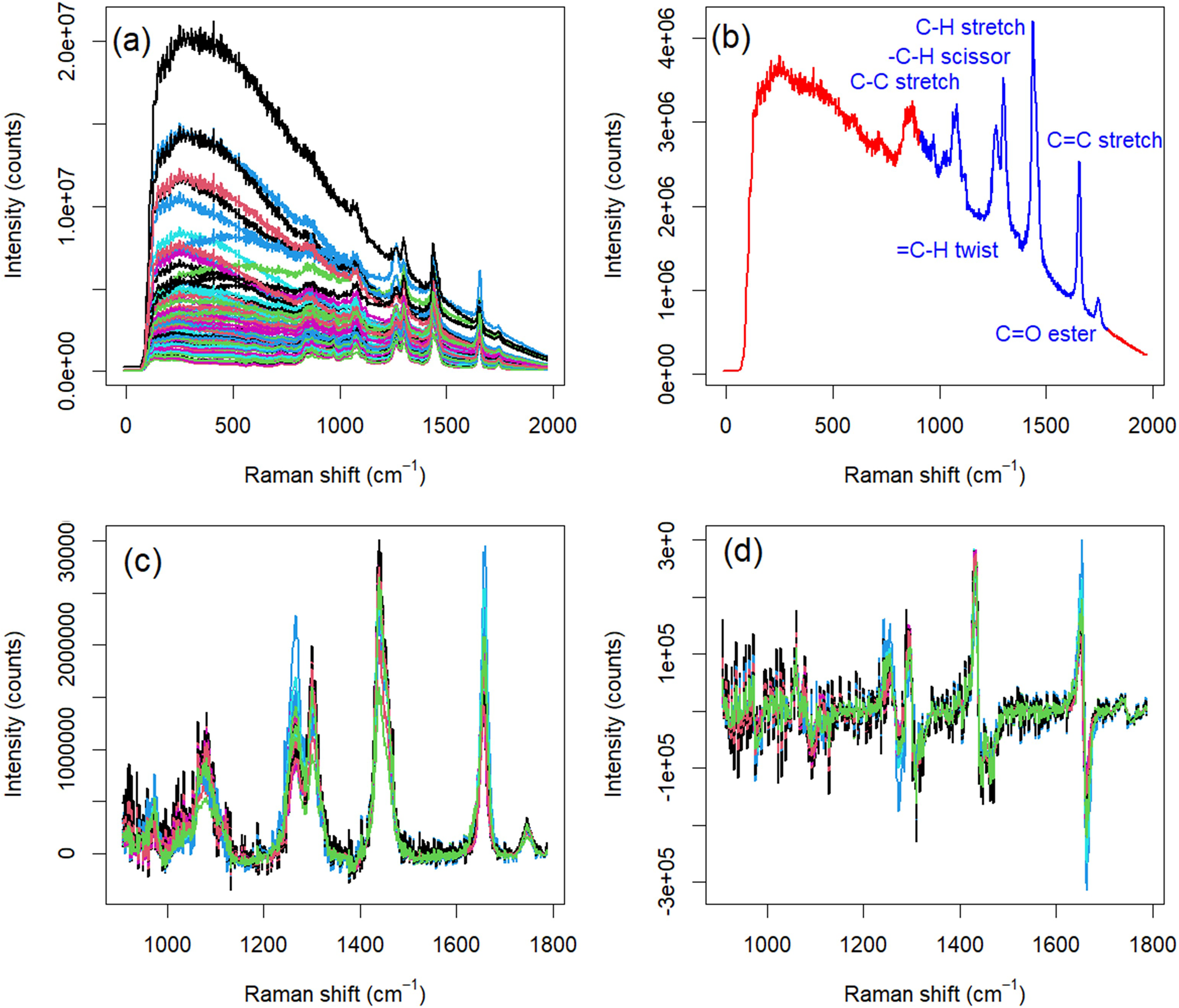
The collected Raman spectra present clear examples where baseline correction is essential for construction of good calibration or classification models. The variance of the informative (Raman) signal is much less than the variance of the uninformative (fluorescence) baseline (Figures 1a and 2a). Additionally, the region from 0 to 1000 cm⁻¹ contains no discernable Raman bands. While two-dimensional (2D) excitation–emission matrix fluorescence spectroscopy has been employed to characterize edible oils,^40,41 one-dimensional (1D) emission fluorescence lacks the information density to differentiate among types of edible oils or to determine the oil PV. Consequently, the Raman signal must be separated from the uninformative as much as possible prior to building a multivariate model.

Figure 1.

Preprocessing steps for Raman spectra collected with a field-portable spectrometer. (a) The spectra exhibited a significant fluorescent baseline that must be removed. (b) Regions of informative Raman signals were identified (blue); other regions were parsed (red). (c) After baseline correction and variable selection, the Raman signal is more prominent above the baseline. (d) A first-derivative Savitzky–Golay filter was employed to help remove any residual baseline.

Figure 2.

Preprocessing steps for Raman spectra collected with a bread-board Raman spectrometer. (a) The spectra exhibited a significant fluorescent baseline that must be removed. (b) Regions of informative Raman signals were identified (blue); other regions were parsed (red). (c) After baseline correction and variable selection, the Raman signal is more prominent above the baseline. (d) A first-derivative Savitzky–Golay filter was employed to help remove any residual baseline.

The R package baseline ³³ is specifically designed for spectroscopic applications and offers a dozen different algorithms for isolating and removing spectroscopic backgrounds. Each algorithm is based on a different optimization criterion and may perform relatively better or worse for different applications. In our experience, the asymmetric least squares (ALS) algorithm ⁴² tends to be the most universally robust for Raman and laser-induced breakdown spectroscopy applications without requiring fine-tuning of the method parameters. Other baseline correction algorithms may be more appropriate for different spectroscopies. The baseline ALS algorithm is the same method that the PLS Toolbox calls a “Whittaker filter” and is often found in the literature as a Whittaker smoother among other names. ⁴³

The asymmetry in ALS pertains to the algorithm assigning more weight to a negative residual than to a positive residual. Hence, the method determines the spectral baseline by minimizing negative deviations and down-weighting the impact of positive deviations. In ALS, there are two user-adjusted parameters, the rigidity of the estimated baseline (λ) and the weight given to positive deviations (p). Making the λ parameter too large will leave a significant residual background in the baseline corrected spectrum. Setting the λ parameter too small will effectively model the informative signal as part of the baseline, removing much information from the corrected spectrum. Similarly, a large p-parameter will introduce negative regions in the corrected spectrum. An overly small p-parameter generates a baseline that may be overly influenced by a few extreme negative residuals, leading to a baseline estimate that is more highly influenced by random noise.

With the baseline package, the spectroscopic background is estimated and removed with a single line of code:

CorrectedSpectrum < - baseline.als (OriginalSpectrum, lambda = 6, p = 0.05)$corrected

The λ = 6 and p = 0.05 values are package defaults that can be adjusted by the analyst for each application. The baseline.als routine actually returns both the baseline corrected spectrum and the estimated baseline. The “$corrected” suffix tells the program to save only the baseline corrected spectrum.

With regard to the Raman spectra, immediate application of the ALS algorithm fails to adequately remove the fluorescence background from the Raman spectra. Sufficiently decreasing the λ parameter to model the highly curved leading edge of the spectra (i.e., <500 cm⁻¹ in this application) renders the baseline estimate to be so flexible that the Raman bands are also interpreted as part of the baseline and removed. This problem can be circumvented by parsing the highly curved or uninformative spectral regions at low and high Raman shifts and focusing on removing the fluorescent background from only the ∼1000 to ∼1700 cm⁻¹ region that contains Raman bands (Figures 1b and 2b). Using baseline.als default settings presents a reasonable estimate of the baseline corrected Raman spectra (Figures 1c and 2c). It is possible that altering the λ and p-parameters or splitting the Raman region into two or more segments for baseline removal might lead to a better-performing model.

The collected NIR and MIR spectra present two confounding effects that can be mitigated by a similar baseline removal procedure as implemented with the Raman data. There is a baseline variance in these spectra that is less prominent than the baseline variance of the Raman data (Figures 3a–7a). The baseline variance is most prominent in the 8 mm OPL NIR spectra (Figure 4a) and least prominent in the MIR transmission data (Figure 6a). This baseline is more likely from the differential placement of the cuvette in the spectrometer than the natural variation of chemistry that gives rise to the variance in the Raman data baseline. Concurrently, the NIR and MIR transmission data all have regions with absorbance above the linear dynamic range of their detectors (∼2.5–3 AU). Only the MIR ATR spectra are completely below the maximum linear range.

Figure 3.

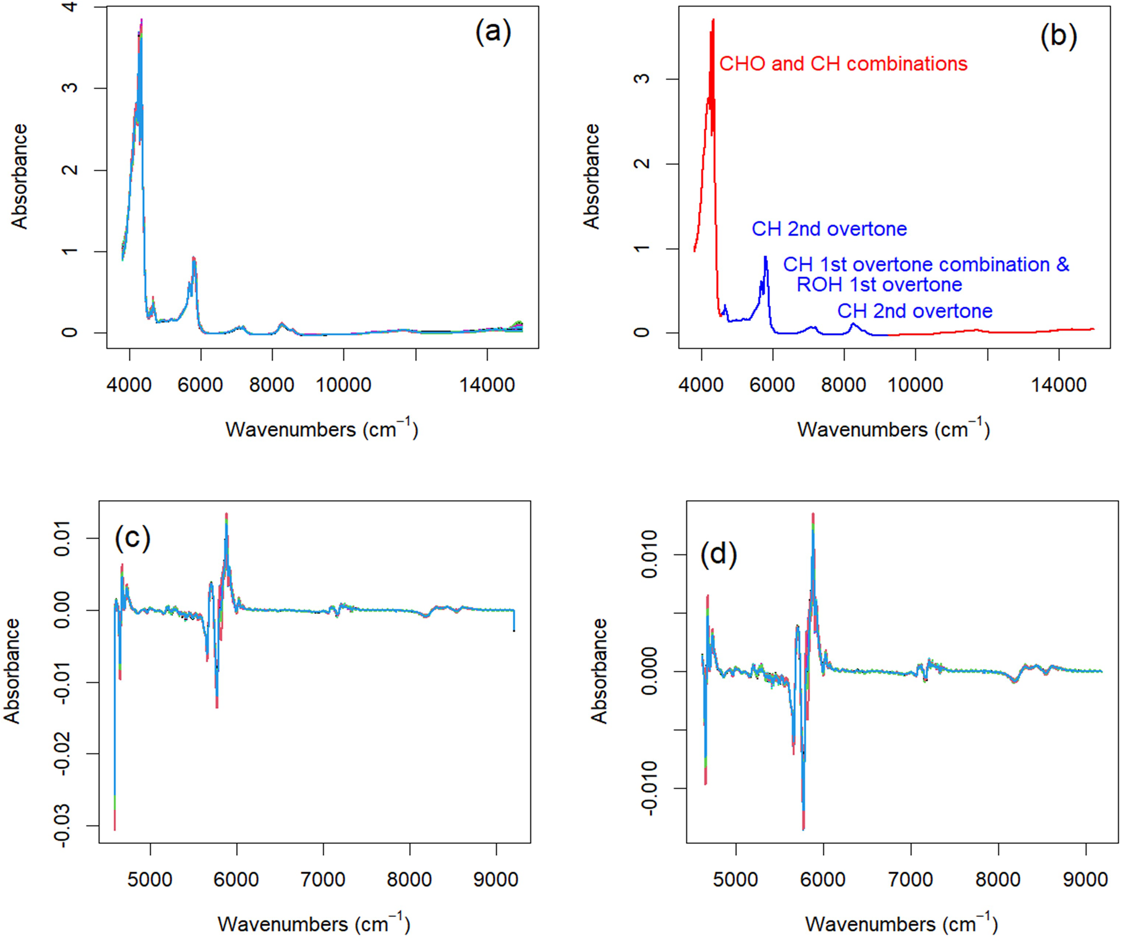
Preprocessing steps for 2 mm OPL NIR absorbance spectra. (a) The spectra exhibit a slight baseline offset. (b) A region of informative NIR absorbance data (blue) was isolated by removing absorbance bands above 3.0 AU and regions of featureless baseline. (c) Treating each spectrum with a first-derivative Savitzky–Golay smoother removed the baseline offset but introduced artifacts on the edges of the region of interest. (d) Truncating the first derivative spectra to remove the edge artifacts produced the spectra used to determine edible oil PV and class.

Figure 4.

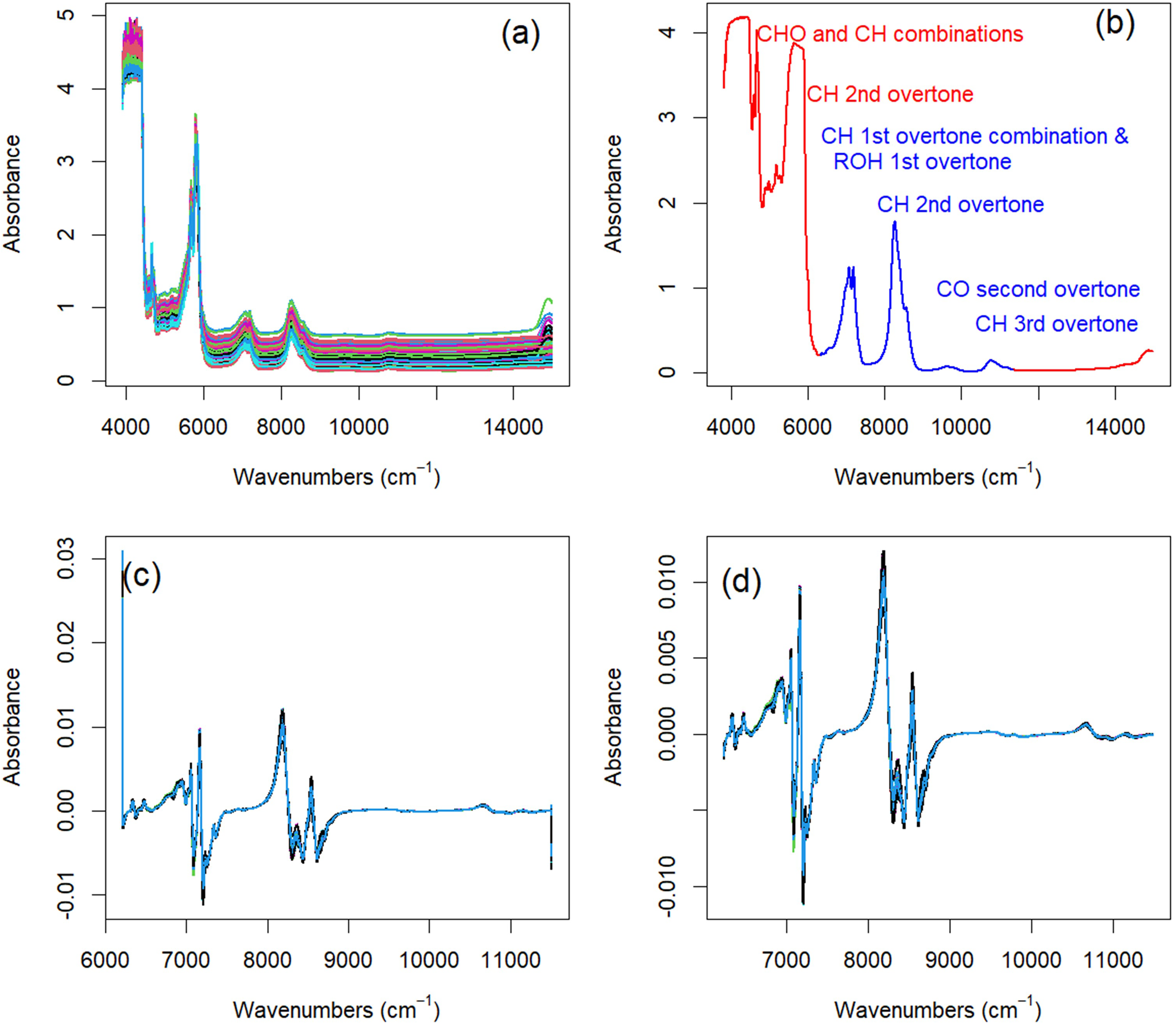
Preprocessing steps for 8 mm OPL NIR absorbance spectra. (a) The spectra exhibit a profound baseline offset. (b) A region of informative NIR absorbance data (blue) was isolated by removing absorbance bands above 3.0 AU and regions of featureless baseline. (c) Treating each spectrum with a first-derivative Savitzky–Golay smoother removed the baseline offset but introduced artifacts on the edges of the region of interest. (d) Truncating the first derivative spectra to remove the edge artifacts produced the spectra used to determine edible oil PV and class.

Figure 5.

Preprocessing steps for 24 mm OPL NIR absorbance spectra. (a) The spectra exhibit a noticeable baseline offset. (b) A region of informative NIR absorbance data (blue) was isolated by removing absorbance bands above 3.0 AU and regions of featureless baseline. (c) Treating each spectrum with a first-derivative Savitzky–Golay smoother removed the baseline offset but introduced artifacts on the edges of the region of interest. (d) Truncating the first derivative spectra to remove the edge artifacts produced the spectra used to determine edible oil PV and class.

Figure 6.

Preprocessing steps for the MIR cuvette-based absorbance spectra. (a) The spectra exhibit a noticeable baseline offset. (b) A region of informative MIR absorbance data (blue) was isolated by removing absorbance bands above 3.0 AU and regions of featureless baseline. (c) Treating each spectrum with a first-derivative Savitzky–Golay smoother removed the baseline offset but introduced artifacts on the edges of the region of interest. (d) Truncating the first derivative spectra to remove the edge artifacts produced the spectra used to determine edible oil PV and class.

Consequently, the presumptive uninformative and malinformative regions of the spectra will be parsed (Figure 3b–7b, red) prior to application of the Savitzky–Golay baseline removal method. ⁴⁴ The Savitzky–Golay algorithm simultaneously smooths the data, reducing the effect of random noise, determining the local derivative of the spectrum, and removing any simple baselines (i.e., baselines that can be approximated as local constant or sloping offsets). Smoothing is accomplished by estimating each point in the spectrum based on a polynomial of fixed order and window length. The baseline is removed by differentiating the polynomial, a first-order derivative removes the constant term, and a second-order derivative removes the linearly sloping baseline. Generally, a second-order polynomial (quadratic equation) is applied. The window length must be an odd integer as the center point is to be replaced with the smoothed value. The optimization of each of the three parameters contains a risk and a reward. Increasing the order of the derivative increases the complexity of the baseline that can be removed. However, this also amplifies the random noise associated with the spectrum. Increasing the order of the polynomial allows for greater fidelity in fitting the spectrum but also amplifies the random noise propagating into the smoothed estimate. Increasing the window width provides better smoothing from greater signal averaging. However, this also increases the risk of spectral distortion if the local data are not well modeled by the polynomial. An accepted rule of thumb is that the Savitzky–Golay window width should be no greater than the width at half-height of the band being smoothed.

With the pracma (PRACtical Math) functions package, Savitzky–Golay smoothing and baseline correction can be achieved with the savgol function. For example, a first derivative of the spectrum from a second-order polynomial with a 5-pixel-wide window is generated with a single line of code:

Spectrum_1D < - savgol (OriginalSpectrum,dorder = 1, forder = 2, fl = 5)

where dorder is the derivative order, forder is the filter (polynomial) order, and fl is the filter (window) length.

For the Raman spectra, a 5-point, first derivative of a second-order polynomial Savitzky–Golay function was applied because the Raman spectra were collected at lower wavenumber resolution than the NIR and MIR spectra. Consequently, there are fewer observations per vibrational band. The inflation of noise with derivatization is evident in the lower signal-to-noise ratio of the derivatized Raman spectra (Figures 1d and 2d) compared to the same spectra prior to the Savitzky–Golay filter (Figures 1c and 2c).

For the NIR and MIR spectra, the leading and trailing regions of no information and misinformation were parsed. Then, a 5-point, first derivative of a second-order polynomial Savitzky–Golay function was applied to mitigate the effects of a constant baseline offset on the calibration and classification model performances (Figures 3c–7c). The implementation of Savitzky–Golay smoothing varies across coded algorithms. Some algorithms parse observations from the leading and trailing edges of the spectra because the Savitzky–Golay algorithm is increasingly extrapolating the polynomial function closer to the spectral edges. The savgol algorithm in the pracma package maintains these observations and leaves the retention decision to the analyst. Parsing these end members returns clean first-derivative spectra with significantly reduced baseline influences (Figures 3d–7d).

Figure 7.

Preprocessing steps for the MIR ATR absorbance spectra. (a) The spectra exhibit a minor baseline offset. (b) A region of informative MIR absorbance data (blue) was isolated by removing regions of featureless baseline at the edges of the spectra. (c) Treating each spectrum with a first-derivative Savitzky–Golay smoother removed the baseline offset but introduced artifacts on the edges of the region of interest. (d) Truncating the first derivative spectra to remove the edge artifacts produced the spectra used to determine edible oil PV and class.

The scaling of the variables (intensity or absorbance at each wavenumber in this case) is applied to adjust the relative weight the calibration or classification models dedicate to the more extreme observations. “Variance scaling", defined as scaling each variable to unit variance, is often considered for spectroscopic applications. Given that many machine-learning optimizations are based on minimizing unmodeled variance, not scaling the variables inherently assigns relative weight (importance) to each variable based on the intrinsic variances. That is to say, a variable that ranges from 0 to 100 will provide more influence on the model than a variable that ranges from 0 to 1. Scaling each variable to unit variance levels the influence of all variables.

Transforming each of the variables to become closer to a Gaussian distribution is a commonly overlooked means of improving model performance. Many statistical and machine learning methods assume a Gaussian distribution of observations within each variable. The further the observation is from the mean, the greater the influence the sample with the extreme (high or low intensity) observation will have on the model. Consequently, variables can be transformed to become closer to a Gaussian distribution to mitigate the influence that a few extreme data points can have on the model. An effective strategy for transforming a variable toward a Gaussian distribution is by a power transformation where the parameter λ is optimized to transform the collection of observations, y, into the more Gaussian distributed y^(λ). The most common of the power transformations is the Box–Cox transformation, ⁴⁵

$$y_i^{(\lambda )}=\{\begin{array}{cc}{\displaystyle \frac{y_i^{\lambda }-1}{\lambda }}& \mathrm{if}\lambda \ne 0\\ \ln y_i& \mathrm{if}\lambda =0\end{array}$$

(1)

However, the Box–Cox transformation does not work with negative observations. Thus, the more generally applicable Yeo–Johnson transformation ⁴⁵ is applied when negative values are present in the spectra,

$$y_i^{(\lambda )}=\{\begin{array}{c}\begin{array}{cc}{\displaystyle \frac{{(y_i+1)}^{\lambda }-1}{\lambda }}& \mathrm{if}\lambda \ne 0,y\ge 0\\ \ln (y_i+1)& \mathrm{if}\lambda =0,y\ge 0\end{array}\\ \begin{array}{cc}{\displaystyle \frac{-{(-y_i+1)}^{(2-\lambda )}-1}{2-\lambda }}& \mathrm{if}\lambda \ne 2,y\ge 0\\ -\ln (-y_i+1)& \mathrm{if}\lambda =2,y\ge 0\end{array}\end{array}$$

(2)

Scaling and transformations should be applied after baseline correction, but before model generation. The exact scaling and transformation parameters applied to the data used to construct the model must be applied to all future samples interrogated by the model. Fortunately, R contains a model-building package that performs requested scaling and transformations and then saves the parameters as part of the model. Consequently, the procedure to implement scaling or transforming of the data will be discussed in the Model construction section below.

Model Preparation

When constructing a calibration or classification model, it is ideal to split the data collection into three unique sets, each set serving a different function. Approximately 60–80% of the data is designated as the training set; all models to be considered, including different permeations of the model parameters, are created with the training set. Approximately 10%–20% of the data collection is used as the tuning set; based on the performance metrics used as model optimization criteria, the best of all models considered is selected by applying each model permeation to the tuning set. The remaining 10–20% of the data form the validation set. The performance metrics of the model when applied to the validation set provide the best estimate of future model performance. The training and tuning sets tend to optimistically estimate model performance because the model was crafted specifically to optimize performance on those two data sets.

In practice, however, there are seldom sufficient collected samples to create three data sets for model training, tuning, and validation. Consequently, the model is tuned on the training set by jackknifing or bootstrapping the performance metrics. Jackknifing and bootstrapping are closely related resampling techniques that estimate the precision of an estimated value. ⁴⁶ Here, the precisions of models’ performance metrics are estimated to determine which models perform the best. Jackknifing and bootstrapping differ in how the training set is resampled and the computationally intensive bootstrapping generally performs better than jackknifing except for small data sets. Leave one out cross-validation (LOOCV) is a particular case of a jackknife while bagging (bootstrap aggregating) is a type of bootstrap.

The caret package (Classification and Regression Training) in R has useful functions for splitting data into training and validation sets and for performing jackknifing or bootstrapping. The createDataPartition function randomly selects a percentage of the data for the training set:

TrainIndicies < - createDataPartition (SampleIndicators, p = 0.8, list = FALSE)

If the SampleIndicators are a vector of numbers (e.g., sample numbers or concentrations associated with each spectrum), the fraction p of the sample collection will be selected. However, if the SampleIndicators are an array of class membership for each sample, the createDataPartition function will assign the fraction p of each class to the training set. This is important for keeping the training and validation sets balanced in class membership during random assignment. The training set and validation set are, hence, readily constructed from createDataPartition:

TrainingSet < - AllData[ TrainIndicies, ]

ValidationSet < - AllData[ -TrainIndicies, ]

where the negative sign (−) indicates all samples not indicated by TrainIndicies.

The trainControl function in caret has 14 different templates to control how jackknifing or bootstrapping will be performed. The simplest

tc < - train Control(method = “LOOCV” )

performs LOOCV. The data in tc will later be passed to the model generation function, train, as discussed in the Model construction section. More control of the resampling procedure can be exerted on the cross-validation option, “cv”, where the training set is randomly divided into number groups and each group is left out once as in LOOCV:

tc < - trainControl (method = “cv”, number = 20)

In the case where number = 20, each group has a unique 5% (1/20th) of the training set. The “repeatedcv” option combines the positive features of both jackknifing and bootstrapping. Repeatedcv performs regular cv multiple times, each with a different random assignment of samples to groups.

tc < - trainControl (method = “repeatedcv”, number = 20, repeats = 10, verbose = TRUE)

In the case where repeats = 10, repeatedcv will aggregate randomly generated 10 cv analyses to estimate the model's performance metric. The final and optional line, “verbose = TRUE", is added for those who like to watch the progress of an iterative algorithm. Because repeatedcv is a good compromise between the accuracy of bootstrapping and the speed of jackknifing, it is a widely employed method for model tuning in the machine learning community.

As a side note, R and RStudio do not perform parallel computing by default. This will make R scripts run slower than their Matlab counterparts, for example, unless R is explicitly told to use the doParallel package. Starting a session with a script such as

require(doParallel)

use_cores < - detectCores() −1

registerDoParallel(cores = use_cores)

assigns all but one of the central processing unit cores to run R functions in parallel. Of course, any lesser number of cores could be dedicated to R, freeing computational power for other tasks. If parallel processing is used, the verbose output setting in trainControl should be set to the default FALSE; the cores cannot talk among each other to explicitly track linear model progress.

Model Construction

The construction and tuning of calibration and classification models are performed by the train function in caret. The caret package is a wrapper that brings together many different packages into a unified syntax to streamline the process of building calibration and classification models. The package supports 284 different calibration and classification methods, only two of which are discussed here as illustrative examples. Each relevant piece of information is passed into the train function and stored in the model for later use when predicting future sample properties with the model. For a calibration application by partial least squares regression (PLSR),

Model_PLSR < - train (x = as.data.frame(Spectra),

y = as.numeric(Property),

preProcess = c(‘center’, ‘scale’),

method = ‘pls’,

tuneLength = 10,

metric = ‘RMSE’,

trControl = tc)

the program knows that calibration, and not classification, is to be performed because the y-input is a numeric vector. Where PLS discriminant analyses (PLS-DAs) are the desired methods, the y-input would be a factor:

Model_PLSDA < - train (x = as.data.frame(Spectra),

y = as.factor(Classes),

preProcess = c(‘center’, ‘scale’),

method = ‘pls’,

tuneLength = 10,

metric = ‘kappa’,

trControl = tc)

Coercing the x-input to be a data frame ensures the file structure of the Spectra matrix is compatible with the train function expectations. The preProcess input lists the preprocessing operations to be performed on each variable; here, the data would be mean-centered and scaled to unit variance. If desired “YeoJohnson” or “BoxCox” could be added to the preProcess() line to transform each variable by an optimized Yeo–Johnson or Box–Cox algorithm to become closer to normally distributed. The method input can be any of the 284 multivariate classification and calibration algorithms supported by caret. For example, method = “svmLinear", would model the data with a linear kernel support vector machine (SVM). The tuneLength, or more generally tuneGrid, is unique to each method. In the case of pls, the algorithm tunes over the number of intrinsic components used. In the case of tuneLength = 10, up to a 10-component model will be considered. The trControl input references the saved trainControl parameters that are needed for tuning the model parameters.

The tuning metric that is chosen to assess model performance forms a key difference between calibration and classification models. The root mean squared error (RMSE) is commonly used to optimize calibration models (“method = RMSE”) while accuracy is commonly used for classification models (“method = Accuracy”). However, the caret package also offers the correlation coefficient between the true and estimated values as a calibration assessment option (“method = Rsquared”) and Cohen's kappa ⁴⁷ as an option for assessing classification (“method = kappa”). For assessing calibration models, RMSE is superior to the correlation coefficient because the correlation coefficient is biased toward estimating extreme samples when an unbalanced training set is used for model development.

Similarly, Cohen's kappa is superior to accuracy for assessing model performance because accuracy is biased to inflate performance metrics with unbalanced training sets. Consider a binary classification {A, B} with p_A = 0.90 and p_B = 0.10. Where “A” guessed 90% of the time, the expected accuracy would be (0.90)(0.90) + (0.10)(0.10) = 0.82. That is to say, a model that provides no information added over random guessing would expect to yield an accuracy of 0.80. Cohen's kappa (κ) accounts for the expected accuracy,

$$\kappa ={\displaystyle \frac{p_o-p_e}{1-p_e}}$$

(3)

by subtracting the expected probability of a correct class assignment, p_e, from the observed probability of a correct class assignment by the model, p_o. The 1 − p_e term normalizes κ to be between 1 for completely correct classification and −1 for completely incorrect classification. A κ of 0 indicates the model is equivalent to random guessing. Kappa values will always be less than accuracies unless the model is perfect (e.g., Figure 8, solid versus dashed lines).

Figure 8.

Cohen's kappa (solid) and accuracies (dashed) for repeated k-folds cross-validation of a PLS-DA model to distinguish olive oil samples from non-olive oil samples by Raman spectroscopy. The cross-validation was performed seven times, each with a different random seed to determine partitions into the training/validation sets and to determine partitions of the training set into k-folds. While the particulars of each repeat are different, the overall trends are consistent.

Model Tuning

Regardless of the model assessment metric, choosing which model parameters are “best” is as much an art as a science. Parameter choice is influenced by two guiding principles: select the model with the best performance metric score, and simple models are better than complex models. The second rule is often referred to as Occam's razor or the parsimony principle. In practice, there are three strategies for identifying the best-performing model:

select the global optimum of all models considered;

organize the models in order of complexity, then select the first local optimum of the ordered model set; and

organize the models in order of complexity, and then select the first model of which there is no statistical improvement in performance when advancing to a more complex model.

Each of these strategies has an inherent set of concerns. The “complexity” of a model is intuitive with factor analysis-based models where adding an additional term increases the model complexity. However, “complexity” does not necessarily describe the impact of optimizing a cost function, e.g., with SVMs or with ridge regression. Additionally, when a model has two or more parameters, how the complexity introduced by one parameter is weighed relative to the complexity introduced by another parameter is not obvious. Statistical methods are problematic due to the difficulty and uncertainty in estimating degrees of freedom. Large data sets may be susceptible to “p-hacking”, having trivial differences be statistically significant due to high degrees of freedom. Consequently, caret avoids these concerns by default selecting the absolute global minimum RMSE (or maximum kappa for classification) of all parameter combinations tested, even though this strategy can lead to overfitting of model parameters and an overly optimistic assessment of model efficacy. However, the analyst can override the default selection and choose the set of model parameters based on any selection criteria.

The range of optimized parameters indicated by the three selection methods is evident in performing repeated k-fold cross-validation, with 10 folds and five repeats to a PLS-DA model tasked with differentiating olive oils from non-olive oils analyzed using Raman spectroscopy. Partitioning a random 20% of the 99 samples into the validation set and performing repeated k-fold cross-validation on the remaining 80 samples indicates three potential optimal numbers of factors (Figure 8, black). The global maximum kappa of 0.9315 occurs at 14 factors. The first maximum occurs with four factors with a kappa of 0.8948. However, the kappa of 0.8938 at three factors is not statistically worse than the kappa of 0.8948 at four factors. The standard deviations of each kappa for the cross-validation are between 0.11 and 0.15, so the kappa must differ by ∼0.05 to be statistically significant at p = 0.5. (Model.name$results returns the optimization metrics and their standard deviations; for 10 folds with five repeats, the kappa will be estimated 50 times.) In the absence of a clearly superior model and because a kappa of 0.89 is not appreciably worse than a kappa of 0.93, a simple model with three or four factors is the most easily justified.

While the optimal model parameters determined by the three selection strategies may differ, it is important to realize that the values of the assessment metrics will also change with the random distribution of samples between the test and validation sets and the random selection of samples within the cross-validation calculations. Consequently, it should be remembered that there is a degree of uncertainty in the optimized model parameters. Repeating the 10-fold with five repeats of cross-validation six times, each with a different random partitioning of the training/validation sets and a different random seed for the cross-validation returns an array of optimized model parameters (Figure 8). The global maximum for kappa spans the range of 11–20 factors, {15, 20, 11, 14, 18, 14, 15}, for seven models. The first maximum ranges from 3 to 5 factors, {4, 3, 5, 5, 4, 3, 4}, for the seven models. However, the first model with no statistical improvement from adding complexity prescribed three factors, {3, 3, 3, 3, 3, 3, 3}, for each of the seven models. Consequently, the decision to use three or four factors is further bolstered by rerunning the model with different permutations of the test/validation set. To override the default choice of parameter optimization by caret, the train function is rerun with

tuneGrid = expand.grid(ncomp = 3)

replacing

tuneLength = 20

The “tuneGrid = expand.grid()” command is more general in that it can handle multiple tuning parameters, and the grid of values is determined by the analyst. In the case of PLS-DA, the number of components (ncomp) is the only tuning parameter and is set to 3.

Tuning a linear SVM discriminant analysis (SVM-DA) model is similar to tuning the PLS-DA model. In the train function, the method must be set to “svmLinear”, and the tuning grid must be specified:

Model_SVMDA < - train(x = as.data.frame (Spectra),

y = as.factor(Classes),

preProcess = c(‘center’, ‘scale’),

method = ‘svmLinear’,

tuneGrid = expand.grid(C = c(1e-5, 0.0001,0.001,

0.01, 0.1, 1, 10)

metric = ‘kappa’,

trControl = tc)

in which PLS-DA tuned over the number of components, the linear SVM function tunes over a cost function, C. Investigating a cost grid running from 1 × 10⁻⁵ to 10 shows an optimized cost function of 0.1 (Table II). A cost parameter C = 0.1 was chosen as optimal because it corresponded to the global maximum kappa of 0.9285, which is also a reasonable estimation of how well the model is expected to perform. Choosing the cost parameter based on the first local maximum kappa would yield a cross-validation kappa of 0.000, which is a model that is literally no better than random guessing.

Table II.

Accuracy and kappa for a linear SVM-DA model tuned over the cost function, C.

C	Accuracy	kappa
1 × 10–5	0.5754	0.0000
5 × 10–5	0.5660	–0.0154
1 × 10–4	0.9188	0.8414
5 × 10–4	0.9131	0.8301
1 × 10–3	0.9131	0.8301
1 × 10–2	0.9512	0.9037
1 × 10–1	0.9637	0.9285
1 × 100	0.9637	0.9285
1 × 101	0.9637	0.9285

The model was constructed to predict whether a sample was olive oil or not olive oil based on Raman spectroscopy.

To train a calibration model to predict PV as a function of vibrational spectroscopy, the y-value in the train function must be designated as a numeric value and the metric must be designated as either “RMSE” or “Rsquared.” The model is tuned over the calibration parameters analogously to how the model is tuned for classification with the exception that RMSE is to be minimized while the other metrics are to be optimized.

Plotting the tuning metric as a function of the tuning parameter can provide comparative insight into analytical performance, comparing either models or spectroscopies. Consider the determination of PV by both PLSR and SVM regression (SVMR) applied to NIR, 24 mm OPL, absorbance data, and MIR absorbance data. For PLSR, NIR both requires a simpler model (global minima at five factors vs. 14 factors) and provides a more accurate estimation of PV, or RMSE of 6.18 versus 7.84 PV (Figure S1a, Supplemental Material). At the same time, SVMR requires a lower cost function for the 24 mm OPL NIR data than the MIR data (cost function of 0.001 vs. 0.1) and the SVM model on the NIR data performs better than the SVM model on the MIR data, RMSE of 5.48 versus 6.60 PV (Figure S1b, Supplemental Material). Comparing all the cross-validation, RMSEs indicate that SVMR would outperform PLSR for PV determination for both data sets.

Prediction of Future Samples

Whereas cross-validation metrics on the training set to tune the model provide a good estimate of future model performance, applying the tuned model to a validation set of samples that are representative of future samples to be analyzed is a superior model benchmark. In the caret package, future samples are interrogated by the predict function:

PredictedValues < - predict(

ModelName,as.data.frame(FutureSpectra)

where the named model stores all the needed preprocessing for the future spectra that were indicated in the train function.

Using the validation set, the model can be assessed numerically and visually. Numerically, if the validation set spans the space of the training set and the model is not overfitting the data, then the RMSE of the model (both RMSE from CV and RMSE from fitting the model to the training set) should be close to the RMSE of the validation set. If the RMSE of CV or fitting is significantly less than the RMSE of prediction, it indicates that the model might have “overfit” the data and is making predictions based on spurious signals that are unique to the training set. An RMSE of prediction less than the RMSE of CV or fitting the model to the training set is an indication that the validation set might not span the sample space of the training set.

The RMSE of prediction can be readily calculated with either the rmserr function in the pracma package or with the rmse function in the Metrics package:

RMSEprediction < - rmserr(TrueValues, PredictedValues)$rmse

with pracma or

RMSEprediction < - rmse(TrueValues, PredictedValues)

with Metrics. The rmserr function actually generates multiple metrics of model quality; the “$rmse” suffix indicates saving just the RMSE. The RMSE of fitting the model to the training set can be determined by using the y-value input into the train function and the predict function on the original training spectra:

FitTrainValues < - predict(ModelName,as.data.frame(TrainSpectra)

RMSEcalibration < - rmse(TrueTrainValues, FitTrainValues)

The model performance can be visually checked by plotting the predicted values against the true values for both the training and validation sets:

plot(TrueTrainValues, PredictedTrainValues,type = ‘p’, pch = 19, col = ‘blue’)

points(TrueValidationValues, PredictedValidationValues,pch = 19, col = ‘red’)

lines(c(−20,1000), c(−20,100), lty = 1, col = ‘black’)

The first line plots samples in the training set as blue dots. The second line overlays samples in the validation set as red dots. The third line of code plots a 1:1 equivalency line for reference.

As expected, the RMSE for cross-validation (RMSECV) is greater than the RMSE for calibration (RMSEC) for both PLSR and SVMR with each spectroscopic technique (Table III). RMSEC is generally lower than RMSECV because RMSEC always decreases as the model becomes more complex. Plus, RMSECV is estimating data points outside of the training subset used at each particular iteration. It is mildly surprising, but not extraordinary, that the RMSE prediction (RMSEP) for the 24 mm OPL NIR data is so much lower than the RMSEC and RMSECV; with relatively small data sets such as these, this could be a random chance in assigning easier-to-predict samples to the validation set. The scenario with the MIR data is more common where the RMSEP is greater than the RMSEC and approximately equal to the RMSECV.

Table III.

Performance metrics for PLSR and SVM calibration models to determine PV with NIR and MIR spectra data sets.

	24 mm OPL NIR		MIR
	PLSR	SVMR	PLSR	SVMR
RMSE calibration (model fit)	5.33 PV	4.90 PV	4.59 PV	4.13 PV
RMSE cross-validation	6.12 PV	5.48 PV	7.23 PV	6.60 PV
RMSE prediction	4.43 PV	2.37 PV	5.96 PV	6.44 PV

Plotting the predicted versus the measured PV provides further insight into the model performances (Figure S2, Supplemental Material) Across both models and both spectroscopies, there is no trend in model fit as a function of PV; low PV samples are modeled comparably to high PV samples. And, importantly, the models estimate the validation samples (red) as well as the models fit the training samples (blue). The similarity in the PLSR and SVMR plots shows that both calibration methods struggle to predict the same samples. The PLSR model presents what might be shown as a Gaussian distribution of model errors in comparison to SVMR where most model and prediction errors are small and a few samples (∼15%) inflate the RMSE. This observation is most evident in the 24 mm OPL NIR plot (Figure S2b, Supplemental Material). In total, the RMSEs and the error plots do not present obvious concerns about the structure or performance of the models.

For classification applications, confusion matrices provide a good means to visualize model performance. The kappa values, such as RMSE, only provide a metric of overall model efficacy. The confusion matrices articulate which classes are well predicted and which classes are often confused with each other. The confusion matrix is a square matrix indexed by the true class categories in each row and the predicted class categories in each column. A perfect classification would, hence, yield a diagonal confusion matrix. For data sets with many classes, confusion matrices might become hard to visually interpret. In such cases, presenting the confusion matrix as a directed network graph could prove beneficial. ⁴⁸ However, with the small number of classes considered in the examples presented here, the confusion matrices are easy to interpret. The confusionMatrix function in caret generates a confusion matrix for the applied model along with a number of summary statistics for the data:

confusionMatrix(PredictedClasses, TrueClasses)

As with regression models, the predicted classes can be obtained through the predict function in caret,

PredictedValues < - predict(ModelName, as.factor(Spectra))

where the spectra can come from either the validation or training sets, for example.

Both PLS-DA and SVM-DA work well for discriminating between olive oil and non-olive oil samples analyzed using Raman spectroscopy. PLS-DA presents a kappa of 0.924 for the training set and a perfect classification for the validation set. SVM-DA performed slightly better with a kappa of 0.962 for the training set and a perfect classification for the validation set. A perusal of the confusion matrices shows that the PLS-DA model misclassified one olive oil training sample as being not-olive oil and one not-olive oil sample as being olive oil (Table IVa). Concurrently, SVM-DA only misclassified one olive oil sample as being a non-olive oil sample (Table IVb).

Table IV.

Confusion matrices for prediction of olive oil (OO) versus not olive oil (Not OO) using (a) PLS-DA and (b) SVM-DA applied to Raman spectra of the edible oils.

(a) PLS-DA model			(b) SVM-DA model
	OO true	Not OO true		OO true	Not OO true
OO Pred.	44, 12	1, 0	OO Pred.	44, 12	0, 0
Not OO Pred.	1, 0	34, 7	Not OO Pred.	1, 0	35, 7

Each entry presents the number of instances in the training set and in the prediction set, separated by commas.

Additional Comments on Classification

Most classification problems are much more complex than a simple binary decision. A typical classification challenge will present three or more classes to differentiate among. These challenges are met by applying one of three modeling strategies, each with a unique set of advantages and concerns:

One versus all (1vAll) models are binary decisions where the target class is differentiated from all other classes as a single group. For a collection of N classes, N models, one for each class, are developed (Figure S3a, Supplemental Material).

Flat models build a single model that distinguishes among all N classes at once (Figure S3b, Supplemental Material).

Hierarchical decision trees divide the classification problem into a series of binary or flat models based on natural groupings of the data (Figure S3c, Supplemental Material). If one node of the hierarchical decision tree has more than one class, that group is isolated, and a subsequent model attempts to distinguish among those classes. This process continues until all classes are either isolated or it is determined that certain groups of classes cannot be distinguished.

Flat classifiers have the advantage of being the most direct path to differentiating among multiple sample classes. However, the classes are often too overlapped or are arranged in the pattern space in such a manner that a single model cannot resolve all classes simultaneously. Binary 1vAll models focus on resolving an individual class from all the others and often can do so with greater accuracy than a flat classifier. However, multiple models must be built and later each assessed using future samples. As with flat classifiers, the 1vAll models may struggle to discriminate classes near the center of the pattern space when the target class cannot be easily separated from the other classes. Additionally, multiple models can lead to ambiguity when the different models assign a particular sample to different classes. Hierarchical classification methods break down complex classification problems into a series of tractable steps. The advantage of hierarchical classification methods is that they can solve problems that are too complex for 1vAll or flat classifiers. The drawback of hierarchical decision trees is that model uncertainty rapidly propagates with the increasing complexity of the tree. Consequently, flat or 1vAll models are preferable to hierarchical models when these simple models work.

Additional Comments on Spectroscopy Choice

Application of a flat PLS-DA or a flat SVM-DA model to distinguish a selection of four oil types (olive, corn, grapeseed, and canola) using Raman spectroscopy (sample set 1A) each provides a good model (Table S2, Supplemental Material). Both algorithms yield an RMSECV kappa of ∼0.93 and a validation set kappa of 0.843. While 0.843 might seem low, this value corresponds to one grapeseed oil sample being misclassified as corn oil in the validation set. Similarly, one grapeseed oil was misclassified as corn oil when the model was fit to the training set.

Additional Comments on Method Validation

The majority of chemometric and machine learning methods are designed to work with “thin” data where there are many more observations than variables and the variables are largely independent of each other. However, spectroscopic data are usually “wide” with many more highly collinear variables than observations. This collinearity in the collected data can lead to “overfitting” of the model to the training data by basing the model on chance correlations within the error structure instead of systematic variance in the variables. For this reason, it is essential to have a “validation” set of observations that span the space of the training set but are completely independent of any sample used to train or tune the model. In practice, observing significantly superior model performance on the training set, relative to the model performance on a well-crafted validation set, is an indication that the model may be overfitting the training set. Consequently, model performance on the validation set should preferably be considered as the indicator of model quality, not model performance on the training set.

Additional Comments on Future Work

There are limitations to this study, as presented here, that should be considered with respect to the design of future studies with this data or for similar analysis campaigns. First, we were limited in the experimental design by restricting the study to commercial edible oils. We wanted to build regression models for both PV and hydroxyl value (HV). The HV is a measure of free hydroxyl groups present in fats and oils and is indicative of the extent to which esterification reactions can occur in edible oils. However, initial titrations showed little variance in the HV across the oil samples because commercial oils are pH stabilized prior to bottling. Oils earlier in the production process would be needed to model HV. We were additionally limited in the number of unique sources of different oils based on commercial availability. Scores of olive oil brands are readily available at local markets, but there are relatively fewer suppliers of nut oils, for example. Consequently, the sample space of the more exotic oils was not as well defined as with the more common oils.

A more extensive study would allow for exploration of more modeling methods. We limited previous studies to linear methods such as PLS, ridge, and least absolute shrinkage and selection operator methods due to the relatively modest collection sizes.^22–25 There are plenty of other regression and classification methods in the caret package (or on other platforms) that could be tested. Random forests, gradient-boosting machines, and artificial neural networks often offer improved model performance at the expense of decreased model interpretability. However, these methods generally require more observations than linear methods to avoid overfitting the model to the data. Perhaps one of the nonlinear methods would outperform the linear methods tested. With a big enough collection of data spanning many brands across harvesting locations and multiple years, deep learning may prove to be the preferred mode of modeling.

Many instrumental methods are impacted by a varying background that is additive to the chemically relevant signal. Separation of the background from the chemical signal, or at least mitigation of the deleterious effects of the background on the model, is broadly referred to as “baseline correction". Unfortunately, there is no good procedure to predict which baseline correction method, with associated parameters, will work best with any application. It is difficult to remove all the background without distorting the chemical signal. Here, we presented a sample of baseline correction strategies that generally work well for Raman and IR spectra in our experience. However, other baseline correction methods may work better for other instrumental techniques or Raman and IR spectra collected with different sample matrices. Ultimately, baseline correction is an exercise of trial and error until one determines a toolbox that generally works well with a particular application.

Additionally, the potential advantages of data fusion have not been fully investigated with this application. Fusion of the 8 mm NIR spectra with the 24 mm NIR spectra did not show improvement in PV prediction relative to using only one data set or the other. ²⁴ The Raman data were viewed as sufficiently poor at estimating PV such that fusion of NIR or MIR with Raman was not attempted. However, other fusion pairings may prove beneficial for PV determination, and fusion of Raman and IR data may prove beneficial for classification.

The successes and challenges of the flat classifier model are reflected in the 1vAll models. The 1vAll models are perfect for olive oil and canola oil but struggle to distinguish corn oil from grapeseed oil when olive and canola oils are present in the model. Adopting a hierarchical decision tree approach, where olive oils and canola oils are first identified and removed from the model, leaves only corn oil and grapeseed oil to be separated. A three-factor PLS-DA model distinguished between these two oils with a kappa of 0.843 for model fit (one misclassification), a kappa of 0.600 for CV, and perfect classification of the validation set with two corn oil and two grapeseed oil samples. The relatively poor CV performance compared to model fit, and validation is often an issue with small data sets. Extracting just the corn oil and grapeseed oil samples presents only 17 samples for the training and validation sets. Assigning four samples to the validation leaves 13 for training. During CV, 10% (one or two samples) are removed with replacement at each iteration. The base assumption of jackknifing is that the space of the model is relatively unchanged when the samples are removed. The low CV metric, compared to fit and validation, is an indication that this assumption does not hold. Consequently, although the model does look promising, assembling a larger training set would be advised before much faith is placed in the model's performance.

A binary classification of olive oil versus non-olive oil with the 24 mm OPL NIR data (sample set 1B) presents less success than the comparable binary classification with Raman on sample set 1A. PLS-DA returned a cross-validation kappa of 0.871 and a validation set kappa of 0.791 while SVM-DA returned a cross-validation kappa of 0.905 and a validation set kappa of 0.947. However, a flat classifier worked better with the NIR spectra than with the Raman spectra. A nine-factor PLS-DA model had a CV kappa of 0.951 with perfect performance for model fit and validation.

Conclusion

This collection of edible oil vibrational spectra provides a good data set for the demonstration and testing of multivariate calibration and classification methods. Deeper analyses and understanding of the edible oil spectra can be found in previous publications.^22–27 The data analysis roadmap laid out in this work can serve as an educational template for exploration of multivariate models applied to other data collections. At the same time, the presented data sets can serve as a test bed for comparison and benchmarking of new multivariate techniques.

The accessibility of facile and inexpensive software is a roadblock to the wider incorporation of advanced chemometric and machine learning tools in spectroscopic research. GUI-based platforms are prohibitively expensive for most classroom and teaching lab settings. Most commercial GUI platforms offer only a limited range of implemented methods. R and RStudio freely offer state-of-the-art multivariate analysis tools with a streamlined mode of implementation, any of the 238 calibration or classification models supported by the caret package in R can be tested by modifying the inputs for caret's train function. Shifting the educational resources and focus from providing limited access to GUI-based software toward developing expertise in an R-based programming environment appears to be successful in our undergraduate and graduate courses.

Supplemental Material

sj-docx-1-app-10.1177_27551857251340426 - Supplemental material for Classification and Peroxide Value Prediction of Naturally Aged Edible Oils Using Raman and Infrared Spectral Analysis

Supplemental material, sj-docx-1-app-10.1177_27551857251340426 for Classification and Peroxide Value Prediction of Naturally Aged Edible Oils Using Raman and Infrared Spectral Analysis by William E. Gilbraith, J. Chance Carter, Kristl Adams, Isio Sota-Uba, Barry K. Lavine, Karl S. Booksh and Joshua M. Ottaway in Applied Spectroscopy Practica

Supplemental Material

sj-zip-2-app-10.1177_27551857251340426 - Supplemental material for Classification and Peroxide Value Prediction of Naturally Aged Edible Oils Using Raman and Infrared Spectral Analysis

Supplemental material, sj-zip-2-app-10.1177_27551857251340426 for Classification and Peroxide Value Prediction of Naturally Aged Edible Oils Using Raman and Infrared Spectral Analysis by William E. Gilbraith, J. Chance Carter, Kristl Adams, Isio Sota-Uba, Barry K. Lavine, Karl S. Booksh and Joshua M. Ottaway in Applied Spectroscopy Practica