Sage Journals: Discover world-class research

Abstract

Breast microcalcifications are crucial clinical features for breast cancer that remain poorly understood with many present contradicting findings and views. Prior research, which utilized Raman spectroscopy (RS), only focused on the mid-frequency spectral region. In this work, we applied low-frequency RS to three experimental setups, with synthetic calcium oxalate and hydroxyapatite in amorphous and crystalline forms immersed and under varying depths of paraffin wax. When comparing the full spectra at all offsets for the three experimental setups, we found that the defocused microspatially offset setup performed the best with an area under the curve (AUC) of 0.87. Furthermore, it was found that the low-frequency spectral region was optimal for this setup with an AUC of 0.94. Overall, the low-frequency region outperformed the mid-frequency spectral regions for two out of the three experimental setups with the AUC improving by up to 13% from 0.81 to 0.94. This is attributed to the low-frequency Raman region containing order information of the probed solids allowing the amorphous and crystalline forms to be more accurately classified.

Graphical abstract

This is a visual representation of the abstract.

Keywords

Raman spectroscopy spatially offset Raman spectroscopy SORS chemometrics receiver operating characteristic biominerals low-frequency Raman spectroscopy breast microcalcifications

Introduction

Breast cancer is the most common cancer among women with approximately 287 850 new cases of invasive breast cancer and 51 300 cases of ductal carcinoma in situ in the United States in 2023.¹ Breast microcalcifications are calcium deposits within the breast that are considered to be robust indicators of breast cancer.² These are usually picked up during a routine mammogram; however, mammography lacks the chemical sensitivity (SE) to distinguish the two types of microcalcifications.³ These two types of microcalcifications are calcium oxalate (CaOx), predominantly associated with benign lesions, and hydroxyapatite (HA), which is associated with benign or malignant lesions depending on its composition and structure.^4–6 Mammography relies on morphological information to categorize microcalcifications based on an international grading system such as Breast Imaging Reporting and Data System, Madame Le Gal, or rhenium-carbon monoxide (CO)-releasing molecule.^7–11 This is then usually followed up with a biopsy to extract and confirm the diagnosis of the microcalcification(s).¹² However, only ∼30% are subsequently found to be malignant, resulting in unnecessary patient trauma and wasting hospital resources.^13,14 There is a clear need for a complementary noninvasive procedure to classify microcalcifications. Vibrational spectroscopic methods, such as Raman spectroscopy (RS), are candidate technologies for such applications due to their chemical specificity (SP) and nondestructive nature.¹⁵

Raman spectroscopy (RS) is an inelastic scattering process wherein incident photons probe the vibrational modes of the target molecule and induce a net change in polarizability (∂α/∂q), where q is the normal coordinates.¹⁶ This phenomenon results in a transfer of energy between the photon and molecule, exciting the molecule to a virtual energy state.¹⁷ The resulting net loss or gain in photon energy correlates with Stokes or anti-Stokes Raman scattering, respectively.¹⁸ This shift in energies corresponds with discrete vibrational modes of the scattered molecule and hence provides chemical and molecularly specific information about the molecule.¹⁹ Raman scattering is a rare phenomenon that occurs once in every 10⁶–10⁸ Rayleigh scattering events.²⁰ A high-intensity monochromatic source is required to overcome the weak nature of this phenomenon, with lasers being the preferred choice.²¹

Prior groundbreaking research on microcalcifications using RS has focused on the mid-frequency (MF) spectral range, enabling the two types of microcalcifications to be successfully classified with additional information.^22–24 Firstly, that malignancy is inversely proportional to carbonate content and could be measured through properties of the 960 cm^–1 peak, which is supported by Fourier transform infrared spectroscopy.^22,25 Carbonate can substitute into HA at either the hydroxyl (OH⁻) or phosphate (PO₄³⁻) sites corresponding to A- and B-type substitution, respectively.^26,27 For breast microcalcifications, B-type substitution is dominant as the environment is more aligned with its synthetic conditions.²⁸ Secondly, through applying sub-techniques of RS such as spatially offset and transmission RS, these calcifications have been successfully detected and classified at clinically relevant depths.^23,24,29,30

For mid-frequency RS (MFRS; 700 to 1800 cm⁻¹), (∂α/∂q) results from intramolecular vibrational modes of the sample such as bending and stretching of chemical bonds within the molecule.^31,32 Comparatively, low-frequency RS (LFRS; 10 to 400 cm⁻¹) probes the intermolecular vibrational modes of the sample through molecules breathing and rocking against each other, again resulting in a net polarization change.³³ LFRS provides information on the structural characteristics of the sample including crystallinity and solid-state form.^34–36 Additionally, LFRS allows the use of both the Stokes (10 to 400 cm⁻¹) and anti-Stokes (−10 to −300 cm⁻¹) spectra potentially allowing for better classification of the sample.³⁷ In this work, we tested if these two features unique to LFRS outperformed MFRS for discriminating CaOx and partially substituted HA in crystalline and amorphous forms buried under varying depths of wax for three deep LFRS experimental setups. This was achieved in a step-by-step manner to draw attention to and flesh out each finding in a clear and concise manner. First by determining which setup performed the best, before finding the ideal spectral region of that setup and its corresponding optimal offset. We hypothesize that the SE of LFRS to the solid-state form will improve the accuracies of Raman microcalcification analysis.

Experimental

Materials and Methods

Calcium oxalate was prepared via mixing of aqueous calcium chloride and sodium oxalate at room temperature with the precipitate CaOx monohydrate collected by vacuum filtration. HA microcalcifications in amorphous and crystalline forms were produced by chemical synthesis, originally described in Thomas et al.,³⁸ wherein the amorphous forms were obtained via vacuum filtration and drying immediately after precipitation. The crystalline HA forms had an additional step of being placed into a furnace at 800 °C for 2 h before slowly cooling down overnight prior to removal.³⁹ The samples of 0.6F HA in the crystalline and amorphous form were the apatites used in this test system as they have been previously characterized, and the sample 0.6F-HA-Cry was near the middle of the range of crystallinities obtained across the different substitution patterns studied.³⁹

Model calcifications of 100 mg were each separately placed into 2.5 g of molten wax and sank to the bottom before the wax hardened. Additional wax blocks of thickness 2.4, 3.6, 4.6, 6.7, 8, 10.2, and 11.8 mm were produced, with any uneven surfaces flattened to ensure minimal air gaps when stacked. This enabled the imitation of microcalcifications buried under varying depths in tissue, when these wax blocks were placed on top of the calcification samples.

Deep Low-Frequency Raman Spectroscopy

The data were gathered using three different deep spatially offset LFRS (SOLFRS) setups, the defocused microspatially offset LFRS (D-microSOLFRS), free space (FS)-SOLFRS, and fiber optic (FO)-SOLFRS, which will be discussed in more detail below.^40,41 A total of 63 spectra were collected for each of the three calcifications and wax as a reference media, with nine spectra at each depth iteration and triplicate spectra at each offset. The spectra were collected using LightField (Princeton Instruments) with a 1 s exposure time and 300 frames that were averaged. The spectra were calibrated using acquired spectra from sulfur and 2-mercaptobenzothiazole by comparing them to reference spectra from McCreery Research Group (National Institute of Nanotechnology, University of Alberta).⁴²

Defocused MicroSOLFRS (D-microSOLFRS)

The D-microSOLFRS utilized a defocused spatial offset geometry, wherein offsets were applied by adjusting the stage along the optical axis. The 200 mW 785 nm excitation laser (Ondax Inc.) was propagated through BragGrate bandpass filters (OptiGrate Corp.), to clean the laser line through the removal of amplified spontaneous emission.^43,44 The laser light was then focused using a 20× microscope objective (MPLN20X, Olympus) onto the sample with a power of 18–37 mW. The backscattered light passed back through the microscope objective, and then a pair of volume Bragg grating notch filters (Ondax Inc.) were utilized to remove the Rayleigh scattered light before being coupled to an LS 785 spectrograph spectrometer (Princeton Instruments) with a charge-coupled device (CCD) detector (PIXIS 100 BR CCD, Princeton Instruments).

Free Space Spatially Offset Low-Frequency Raman Spectroscopy (FS-SOLFRS)

The FS-SOLFRS utilized a lateral spatial offset geometry wherein offsets were applied laterally via a mirror, which refracted the beam incident upon the sample ∼30° from the optical axis.⁴⁰ The FS-SOLFRS used the same excitation laser, objective bandpass filter, and spectrometer as the D-microSOLFRS, with power at the sample ranging from 68 to 80 mW. The scattered light was propagated through a pair of volume Bragg gratings (Ondax Inc.) before being focused on the spectrometer.

Fiber Optic Spatially Offset Low-Frequency Raman Spectroscopy (FO-SOLFRS)

The FO-SOLFRS probe used the same excitation laser and bandpass filter as mentioned previously, wherein the wavefield was coupled into an FO probe. The FO probe had a three-prong design above the sample with power ranging from 114 to 121 mW and offsets set by changing the output fiber connection. The output optic fiber was connected to a mount in the FS-SOLFRS setup to utilize the notch filters and spectrometer.

Optical Geometry

The D-microSOLFRS and FS-SOLFRS used offsets of 0, 2, and 5 mm, while the FO-SOLFRS was fixed to offsets of 0, 2.5, and 5 mm. The D-microSOLFRS utilized a defocused geometry, as seen in Figure 1, wherein offsets were applied along the optical axis via the stage. This resulted in a change in the accepted volume of scattered photons.⁴⁵ In contrast, the other methods utilized lateral spatially offset geometries, wherein offsets were applied laterally via the mirror for the FS-SOLFRS and changing the connected output fiber for the FO-SOLFRS.⁴⁶ Both these methods enable the retrieval of deep propagating photons, which tend to migrate laterally in a random walk-like fashion as they propagate through a turbid media, with a key distinction.^23,47

Figure 1.

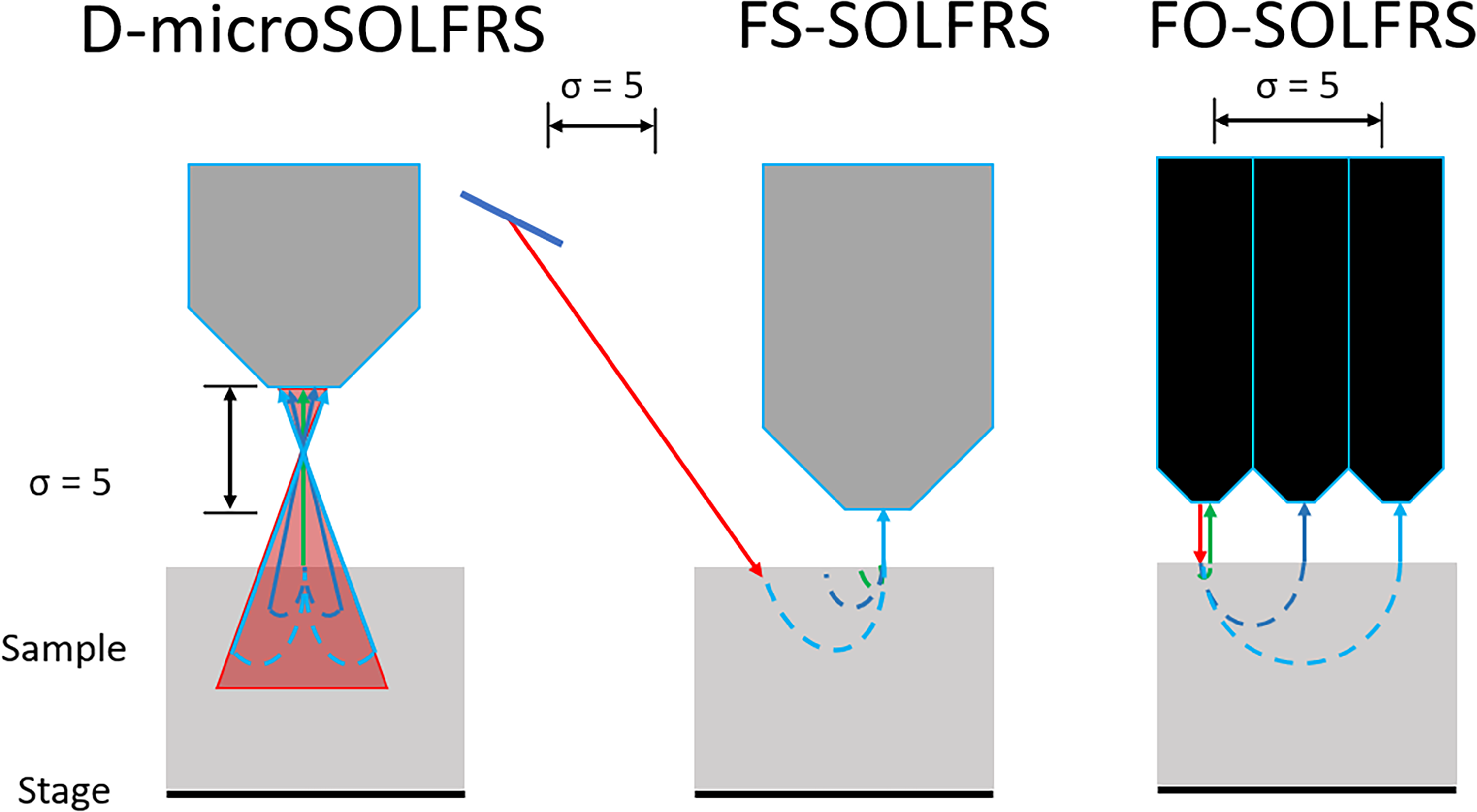
Schematics of the LFRS setups, showing the different geometries and offsets applied denoted by σ (mm). The D-microSOLFRS setup utilized a defocused geometry, wherein applying an offset along the optical axis resulted in an alteration of the volume of accepted scattered photons. The FS-SOLFRS and FO-SOLFRS utilized spatial offsets by adjusting the mirror laterally and switching output fibers, respectively. The key difference between the two geometries was that the defocused geometry does not filter out any of the surface-scattered photons while spatial offset does so at the expense of S/N.

The spatially offset geometry suppresses the superficial or subsurface scattered photons while defocused geometry does not.⁴⁸ This means that with an increasing offset, the signal-to-noise ratio (S/N) will decrease for the spatially offset geometry, but increase for the defocused geometry, at the expense of spatial resolution. Additionally, this means there is an optimal offset for the defocused geometry when the proportion of deeply scattered photons to surface scattered photons is maximized and the proportion of deeply scattered photons to S/N for the spatially offset geometry. One key advantage of microSORS is that it does not require additional reconfiguration with no immediate constraints on the applied offsets.⁴⁹

Data Analysis

Statistical Analysis

Receiver operating characteristic (ROC) curves are produced by varying the decision threshold of the classifier and marking the true positive rate (TPR) and false positive rate (FPR) at each threshold, yielding an empirical ROC.^50,51 This allows ROC curves to assess the performance of the classifier independently of the decision threshold.⁵² These points can be fitted using a binomial distribution yielding a fitted or smooth ROC.⁵³ Empirical ROC curves were used in this work to ensure there was no potential bias induced from fitting the ROC curves.

The area under the curve (AUC) measures the overall performance of the classifier and can be interpreted as the average value of SE over varying values of SP.^54,55 In general, the AUC must be >0.8 to be considered acceptable in a clinical setting.⁵⁶ SE is defined as the proportion of people who are correctly diagnosed with a disease and equivalently is the TPR.⁵⁷ SP is the proportion of people who are correctly diagnosed with not having a disease or the true negative rate (TNR).⁵⁸ Additional statistical rates are the FPR and false negative rate (FNR), respectively, which can be calculated from the “true rates” via FNR = 1 − TPR and FPR = 1 − TNR.⁵⁹ Classification accuracy (CA) is a measure of the proportion of people that are correctly diagnosed as having or not having the disease with respect to the total population tested.⁶⁰

Support vector machine (SVM) classifiers map the data into a higher dimensional feature space set by the kernel to find a line (hyperplane), which successfully separates the data.^61–63 This hyperplane is optimal when the distance between the line and the nearest data point for each class (margin) is maximized.⁶⁴ SVMs are based on statistical learning theory and use structural risk minimization to avoid overfitting the data.⁶⁵ We chose to use an SVM classifier with a radial basis function (RBF) kernel as it performed the best when compared with other classifiers and kernels trialed.^64,66,67

Experimental Analysis

Cosmic spikes with a max pixel width of 5 were removed from the spectra using SpectraGryph.⁶⁸ The data were then imported into Matlab where the data were split into low frequency (LF) and MF spectral regions, ranging from −300 to 400 cm⁻¹ and 700 to 1800 cm⁻¹, respectively.⁶⁹ The spectral region from 400 to 700 cm⁻¹ was observed to be silent and therefore was excluded from the data set. The Raman line was removed from the LF spectra from approximately −20 to 20 cm⁻¹ before the LF spectral region underwent linear baseline subtraction to correct for baseline difference while maintaining the presence of the vibrational density of states.⁷⁰ In contrast, rubber band baseline correction⁷¹ was performed from (700, 1350) and (1350, 1800) in the MF spectral region. All the spectra were normalized using standard normal variate (SNV) to correct for intensity variations within the data gathering procedure.⁷² Finally, both the spectral regions were modeled in a “one-versus-all” approach using an error-correcting output code SVM classifier with an auto-scaled RBF. The classifier was created using the fixed training set and evaluated using the fixed test set samples (Table I).⁷³ The training and test data sets were created with a staggered approach to cover the range of thicknesses and model calcification types in both the training and test data sets. All model performance parameters reported are that of the test set sample set.

Table I.

Sample set measured and the associated training and test set used to construct and evaluate the SVM model.

Depth (mm)	0	2.4	3.6	4.6	6.7	8	10.2
Calcium oxalate	M	M	T	M	M	T	M
Hydroxyapatite crystalline	M	T	M	M	T	M	M
Hydroxyapatite amorphous	T	M	M	T	M	M	M
Wax	M	M	T	M	M	M	T

M, model (training) set; T, test set.

Scaled wax subtraction was performed separately before or after the aforementioned preprocessing procedure on the combined LF and MF D-microSOLFRS data set in Matlab. The spectra incorporated all offsets and thicknesses with the same staggered model and test set used as in Table I, to construct and evaluate the SVM model with the same aforementioned template. This was achieved by first taking the mean of the wax for each offset, then scaling the mean wax spectra based on the 1294 cm⁻¹ peak and multiplying it by 0.9 to ensure no negative features were present in the spectra. This was then subtracted from each spectrum individually. This process resulted in a negligible increase in performance when scaled wax subtraction was performed after preprocessing and a decrease in performance when applied prior to preprocessing.

The first five principal components (PCs) of the same data set under the same conditions were then fed into an SVM with the same template and a one-versus-all linear discriminant analysis model. However, both yielded worse results (see Figure S2, Supplemental Material) and were not further investigated.

Results

Visual Inspection

The mean spectra of the surface calcifications and wax at 2 mm offset are given in Figure 2. All spectra are dominated by the paraffin wax features at 891, 1063, 1133, 1294, 1416, 1441, and 1463 cm⁻¹.⁷⁴ The only discerning feature is the v₁PO₄3⁻ peak at ∼960 cm⁻¹ for the HAs. The other peaks in the MF spectral region are attributed to paraffin wax. The low wavenumber spectral region is dominated by the underlying wax signature with dominant peaks around −90 and 93 cm⁻¹. We see that the calcifications are challenging to distinguish from each other from spectral observation alone.

Figure 2.

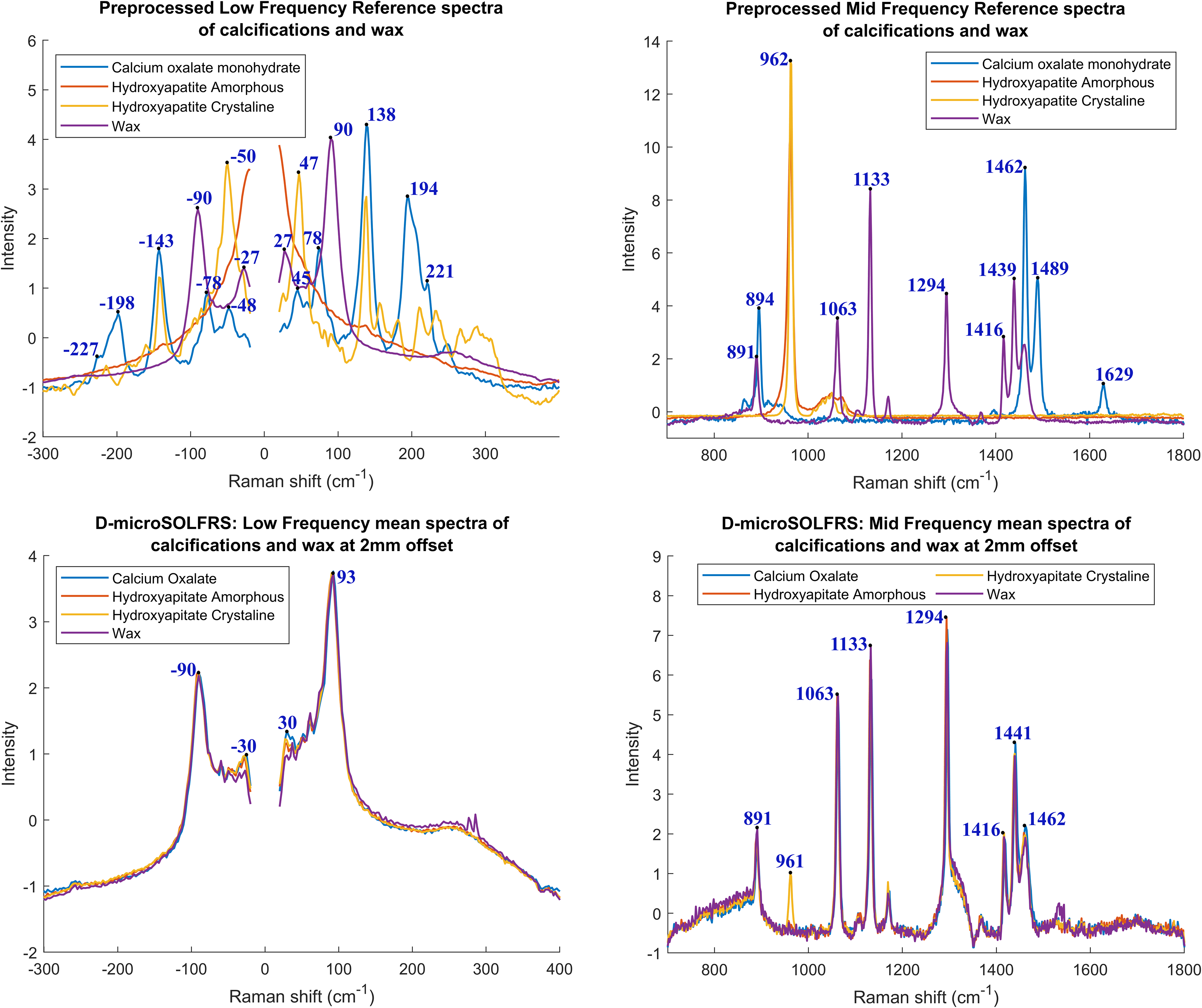
Split and preprocessed reference (top) and mean (bottom) Raman spectra of calcifications and wax from the D-microSOLFRS data set. The spectra were split into LF and mid-frequency (MF) spectral regions spanning −300 to 400 cm⁻¹ and 700 to 1800 cm⁻¹, respectively. The Rayleigh line was removed from the LF spectra before undergoing linear baseline subtraction while rubber band baseline correction was performed for the MF spectral region. All the spectra were normalized using SNV.

Principal Component Analysis (PCA)

Principal component analysis (PCA) was performed on the preprocessed spectra to gain insights into the nature of the data set obtained. The scores and loading of the first three PCs are shown in Figure 3, encompassing 63.6, 6.3, and 3.3% of the respective explained variance. We observe that principal component 1 (PC1) solely encompasses information pertaining to the offset applied to the optical setup. This is highlighted in its respective loading where we see wax features in the positive loadings space, with peaks at −88, 90, 889, 1133, 1418, and 1439 cm⁻¹ (Figure 3c, supported by Figure 2). While in the negative loading space, there are broad features that result from the change in offsets. This enables the offsets to be clearly separated along PC1 (Figure 3a). Focusing on calcification type, we see that no single or combination of PCs appears to accurately separate all four categories (Figure 3b). Calcium oxalate is separated along principal component 2 (PC2), while the others remain clustered together. The PC2 loadings appear to contain HA and blue shifted wax signals in the negative loadings space with its distinguishing v₁PO₄³⁻ peak at 962 cm⁻¹.⁷⁵ Calcium oxalate is apparent in the positive feature space with its unique symmetric and antisymmetric CO stretching with peaks at 1472 and 1635 cm⁻¹ alongside redshifted paraffin wax signal.^76–79 Finally, the loadings for principal component 3 (PC3) contain wax in the positive feature space with peaks at 886 and 1294 cm⁻¹ as well as a shift from 1129 to 1136 cm⁻¹. Crystalline HA is apparent in the negative feature space with defining peaks at −139, −25, 30, 143, and 961 cm⁻¹ (Figures 2 and 3c).³⁹

Figure 3.

Principal component analysis (PCA) of the preprocessed D-microSOLFRS spectra showing the score plots of the first three PCs (a, b) and their respective loadings (c). (a) Score plots for PC1 versus PC2 and PC2 versus PC3 with labeling based on measurement offset. (b) Score plots for PC1 versus PC2 and PC2 versus PC3 with labeling based on buried calcification composition. (c) The associated loading plots for PC1–PC3 describe the nature of variance observed in the score plot.

Optimal Setup

First, to determine the optimal experimental setup, an ROC curve was produced by the fixed test data for the LF spectral regions of the experimental setups incorporating all offsets, as shown in Figure 4. We observe from the ROC that the D-microSOLFRS objective performed the best with the highest AUC of 0.87, as well as the highest CA, SE, and SP, as shown in Tables S1–S3 (Supplemental Material). This was followed by the FO-SOLFRS and FS-SOLFRS setups with respective AUCs of 0.69 and 0.57.

Figure 4.

Receiver operating characteristic (ROC) curve of the experimental setups modeled using SVMs with an RBF kernel. SVMs were modeled using LF spectra from all the offsets obtained for each of the setup sample spectra with a staggered thickness model and test set. We see from the obtained AUCs that the D-microSOLFRS performed the best.

A potential explanation for this is defocused geometry utilized by the D-microSOLFRS, wherein increasing offsets increases the volume of accepted photons, which incorporates deep propagating photons at the cost of spatial resolution. This means that there is no loss in S/N as in spatial offset geometries employed by the other experimental methods and thus allows the D-microSOLFRS to perform the best.

Optimal Spectral Region

We then focused on the D-microSOLFRS as it performed the best and first evaluated performance of LF, MF, and combined frequency spectral regions at all offsets by an ROC, as shown in Figure 5. From this, we see that the LF spectra performed the best with the highest AUC of 0.94 compared to 0.87 and 0.81 for the full and MF spectral regions, respectively. This is due to the LF spectral region containing information about the structural characteristics of the sample including the solid-state form. This information allowed the amorphous and crystalline forms of HA to be correctly classified.

Figure 5.

Receiver operating characteristic (ROC) curve to evaluate the performance of different spectral regions from the D-microSOLFRS experimental setup. The LF spectral region performed the best with the highest AUC of 0.94, as it was able to successfully discriminate between the amorphous and crystalline forms of HA. This is because LFRS probes the intramolecular modes and vibrations obtaining structural information about the sample such as crystallinity and hence excels at separating materials of different (physical/chemical) states.

Optimal Offset

We then evaluated the performance of the 0, 2, and 5 mm offsets for the D-microSOLFRS in the LF spectral region. From the ROC shown in Figure 6, the 0 mm offset performed slightly better than the 2 mm offset with respective AUCs of 0.93 and 0.92.

Figure 6.

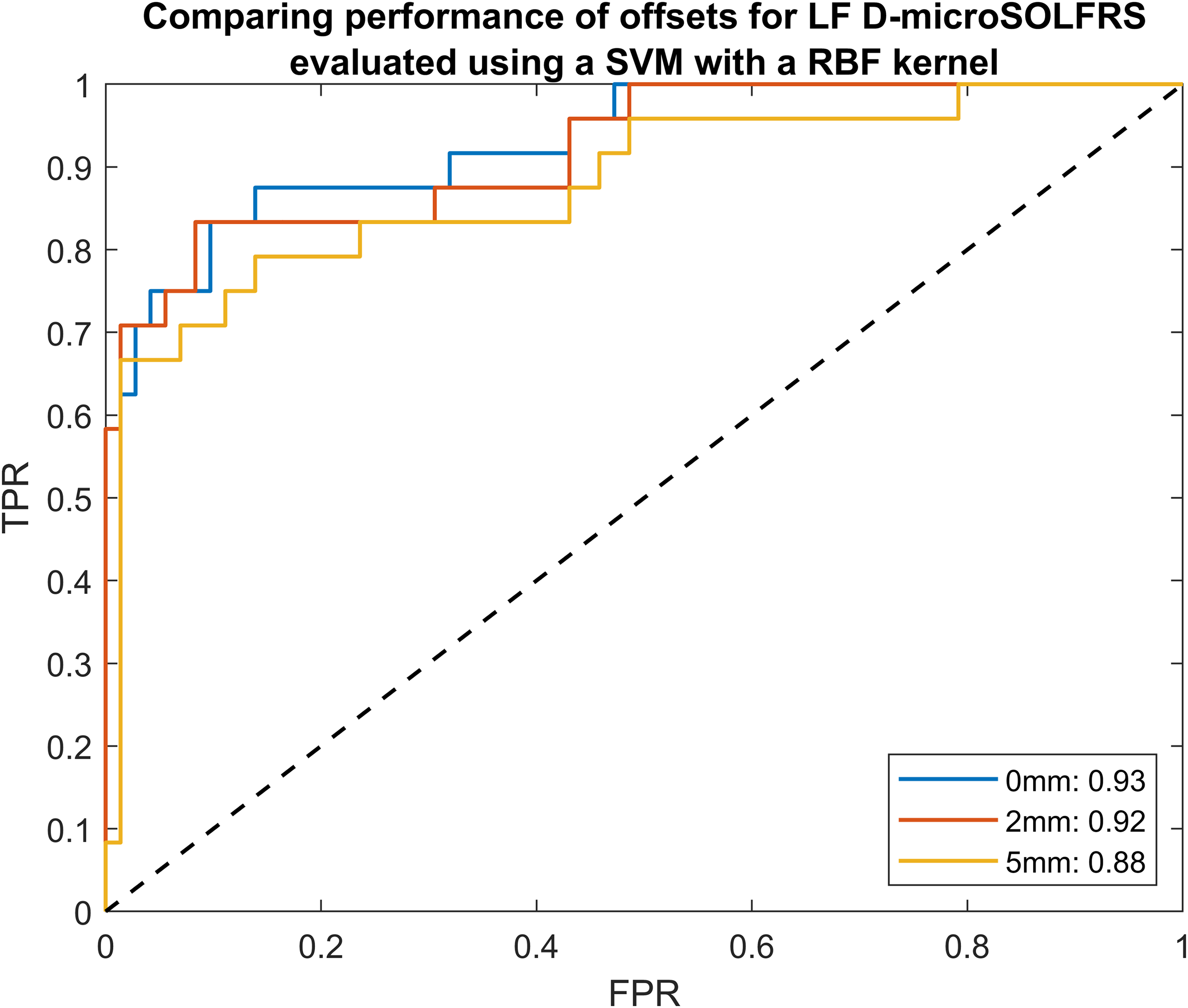
Receiver operating characteristic (ROC) curve evaluating the performance of different offsets from LF spectra obtained in the D-microSOLFRS experimental setup. Even though the 0 mm performed the best, we cannot confidently consider it to be the optimal offset due to the large variation of wax thickness employed in the spectral data set.

However, noting the narrow difference between the 0 and 2 mm offsets, it is hard to conclude that the 0 mm offset is generally optimal. In fact, looking through Tables S1–S3 (Supplemental Material), we see that the best-performing offset varies sizably between experimental setups and their spectral regions. This is due to the variation of wax thickness employed in the spectral data set that ranged from 0 to 10.2 mm. Intuitively, the 0 mm offset will perform best for small wax thicknesses and degrade as it increases, and vice versa for the larger offsets. Therefore, in this case, no optimal offset can be rigorously determined.

Finally, we were interested in determining the best-performing spectral regions for all experimental setups. This was achieved by calculating the percentage difference between the LF and MF spectral regions for all the experimental setups with respect to the model evaluation parameters AUC, CA, SE, and SP (Figure 7), wherein a positive or negative percentage difference corresponds to the LF performing better or worse than the MF spectral region, respectively.

Figure 7.

Bar graph evaluating the percentage differences between the LF and MF spectral regions of the three experimental setups in terms of the model evaluation parameters. We see that the LF spectral region generally outperforms the MF spectral regions except for the FO-SOLFRS data set.

We see that generally, the LF outperforms the MF spectral regions with D-microSOLFRS experiencing the largest improvements in AUC, CA, SE, and SP of 13, 11, 22, and 7%, respectively. FO-SOLFRS is the exception to this trend and could be due to the additional step of removing the signal from the silica glass in the spectra. This was only required and performed on the FO-SOLFRS data set as it was the sole probe utilized in this work. This procedure may have impacted the LF spectral region more than the MF or the silica glass spectra masked important information in the LF spectral region.

Discussion

It is important to note that when applying these models to clinical diagnostic applications, other aspects need to be considered, such as the confirmation test, in this case being biopsy of the microcalcifications. Biopsying the patient results in additional resources spent by the hospital with the patient undergoing mental, physical, and financial trauma.^13,14,80

Recent research on breast microcalcifications has utilized energy-dispersive X-ray, X-ray diffraction, and multimodal imaging approaches as well as RS.^5,12,81–86 As mentioned previously, the malignancy of the cancer is correlated with breast microcalcification composition; however, many of these findings are contested so a brief summary will be given. Firstly, carbonate was shown to correlate with benign lesions; however, the simplicity of this is being challenged as carbonate content can be affected by the surrounding tissue environment.^{5,12,22,25,85} Magnesium, before being confirmed as whitlockite, was initially found to correlate with malignancy; however, more recent studies have found the opposite.^5,28,81–86 Finally, sodium has been found to routinely correlate with malignancy.^5,28,82,84 Future work will focus on incorporating additional samples of HA substituted with varying concentrations of Mg²⁺ or CO₂3⁻ in a more accurate tissue phantom to see if crystalline structural changes from these substitutions can be classified.^28,87,88

Conclusion

Breast microcalcifications are crucial clinical features for detecting breast cancer that remain poorly understood with many present contradicting findings and views. Prior research, which utilized RS, only focused on the MF spectral region. We applied LFRS from three experimental setups to synthetic CaOx and HA in amorphous and crystalline forms immersed and under varying depths of paraffin wax. We found that the LF outperformed the MF spectral regions for two out of the three experimental setups as LFRS contains structural information of the probed molecule. Of the experimental setups, the D-microSOLFRS performed the best with an AUC of 0.87, as it utilized a defocused geometry as opposed to a spatially offset geometry. The optimal performance of the D-microSOLFRS objective was achieved in the LF spectral region with an AUC of 0.94. We have shown the potential of LFRS to accurately classify breast microcalcifications with future research focusing on carbonate and magnesium-substituted HA in hydrogel-based tissue phantoms.

Supplemental Material

sj-docx-1-app-10.1177_27551857241302079 - Supplemental material for Discriminating Model Microcalcifications Immersed and Under Varying Depths of Wax Using Deep Low-Frequency Raman Spectroscopy

Supplemental material, sj-docx-1-app-10.1177_27551857241302079 for Discriminating Model Microcalcifications Immersed and Under Varying Depths of Wax Using Deep Low-Frequency Raman Spectroscopy by Mitchell C. Chalmers, Teemu Tomberg, Keith C. Gordon and Sara J. Fraser-Miller in Applied Spectroscopy Practica

Footnotes

Acknowledgments

Mitchell C. Chalmers thanks the University of Otago for his PhD scholarship.

Declaration of Conflicting Interests

The authors declared no potential conflicts of interest with respect to the research, authorship, and/or publication of this article.

Funding

The authors disclosed receipt of the following financial support for the research, authorship, and/or publication of this article: This work is supported by the Royal Society Te Apa̅rangi, Marsden Fast-Start (Grant No. 19-UOO-210) and Te Whai Ao–The Dodd-Walls Center for Photonic and Quantum Technologies.

ORCID iDs

Mitchell C. Chalmers

Teemu Tomberg

Sara J. Fraser-Miller

Supplemental Material

All supplemental material mentioned in the text is available in the online version of the journal.

References

Siegel

R.L.

Miller

K.D.

Wagle

N.S.

Jamal

. “Cancer Statistics, 2023”. CA Cancer J. Clin. 2023. 73(1): 17–48.

Rominger

Wisgickl

Timmesfeld

. “Breast Microcalcifications as Type Descriptors to Stratify Risk of Malignancy: A Systematic Review and Meta-Analysis of 10665 Cases with Special Focus on Round/Punctate Microcalcifications”. Röfo. 2012. 184(12): 1144–1152.

Obenauer

Hermann

Grabbe

. “Applications and Literature Review of the BI-RADS Classification”. Eur. Radiol. 2005. 15: 1027–1036.

Frappart

Boudeulle

Boumendil

Lin

H.C.

, et al. “Structure and Composition of Microcalcifications in Benign and Malignant Lesions of the Breast: Study by Light Microscopy, Transmission and Scanning Electron Microscopy, Microprobe Analysis, and X-ray Diffraction”. Hum. Pathol. 1984. 15(9): 880–889.

Kunitake

J.A.

Sudilovsky

Johnson

L.M.

Loh

H.-C.

, et al. “Biomineralogical Signatures of Breast Microcalcifications”. Sci. Adv. 2023. 9(8): eade3152.

Radi

M.J.

. “Calcium Oxalate Crystals in Breast Biopsies: An Overlooked Form of Microcalcification Associated with Benign Breast Disease”. Arch. Pathol. Lab. Med. 1989. 113(12): 1367–1369.

Spak

D.A.

Plaxco

Santiago

Dryden

Dogan

. “BI-RADS Fifth Edition: A Summary of Changes”. Diagn. Interv. Imag. 2017. 98(3): 179–190.

Gülsün

Demirkazık

F.B.

Arıyürek

. “Evaluation of Breast Microcalcifications According to Breast Imaging Reporting and Data System Criteria and Le Gal’s Classification”. Eur. J. Radiol. 2003. 47(3): 227–231.

Simonetti

Lattanzio

. “Interpreting and Reporting”. In: Sud

, editor. Mammography: Guide to Interpreting, Reporting and Auditing Mammographic Images. Berlin: Springer-Verlag, 2005. Pp. 255–266.

10.

Frappart

Remy

Lin

H.C.

Bremond

, et al. “Different Types of Microcalcifications Observed in Breast Pathology: Correlations with Histopathological Diagnosis and Radiological Examination of Operative Specimens”. Virchows Arch. A. Pathol. Anat. Histopathol. 1987. 410: 179–187.

11.

D’Orsi

Sickles

Mendelson

Morris

, et al. ACR BI-RADS Atlas: Breast Imaging Reporting and Data System. Reston, VA: American College of Radiology, 2013.

12.

Sathyavathi

Saha

Soares

J.S.

Spegazzini

, et al. “Raman Spectroscopic Sensing of Carbonate Intercalation in Breast Microcalcifications at Stereotactic Biopsy”. Sci. Rep. 2015. 5(1): 9907.

13.

Brewer

N.T.

Salz

Lillie

S.E.

. “Systematic Review: The Long-Term Effects of False-Positive Mammograms”. Ann. Intern. Med. 2007. 146(7): 502–510.

14.

Wilkinson

Thomas

Sharma

. “Microcalcification on Mammography: Approaches to Interpretation and Biopsy”. Br. J. Radiol. 2017. 90(1069): 20160594.

15.

Nicolson

Kircher

M.F.

Stone

Matousek

. “Spatially Offset Raman Spectroscopy for Biomedical Applications”. Chem. Rev. Soc. 2021. 50(1): 556–568.

16.

Raman

C.V.

. “A New Radiation”. Indian J. Phys. 1928. 2: 387–398.

17.

Diem

. “Introduction to Raman Spectroscopy”. In: Introduction to Modern Vibrational Spectroscopy. Chichester, UK: Wiley, 1993. Pp. 109–145.

18.

Pelletier

M.J.

. “Introduction to Applied Raman Spectroscopy”. In: Analytical Applications of Raman Spectroscopy. Oxford, UK: Blackwell Science, 1999. Pp. 1–53.

19.

Butler

H.J.

Ashton

Bird

Cinque

, et al. “Using Raman Spectroscopy to Characterize Biological Materials”. Nat. Protoc. 2016. 11(4): 664–687.

20.

Long

D.A.

. “Survey of Light-Scattering Phenomena”. In: The Raman Effect: A Unified Treatment of the Theory of Raman Scattering by Molecules. Chichester, UK: Wiley, 2002. Pp. 3–18.

21.

Bumbrah

G.S.

Sharma

R.M.

. “Raman Spectroscopy—Basic Principle, Instrumentation and Selected Applications for the Characterization of Drugs of Abuse”. Egypt. J. Forensic Sci. 2016. 6(3): 209–215.

22.

Haka

A.S.

Shafer-Peltier

K.E.

Fitzmaurice

Crowe

, et al. “Identifying Microcalcifications in Benign and Malignant Breast Lesions by Probing Differences in Their Chemical Composition Using Raman Spectroscopy”. Cancer Res. 2002. 62(18): 5375–5380.

23.

Matousek

Stone

. “Prospects for the Diagnosis of Breast Cancer by Noninvasive Probing of Calcifications Using Transmission Raman Spectroscopy”. J. Biomed. Opt. 2007. 12(2): 024008.

24.

Stone

Baker

Rogers

Parker

A.W.

Matousek

. “Subsurface Probing of Calcifications with Spatially Offset Raman Spectroscopy (SORS): Future Possibilities for the Diagnosis of Breast Cancer”. Analyst. 2007. 132(9): 899–905.

25.

Baker

Rogers

Shepherd

Stone

. “New Relationships Between Breast Microcalcifications and Cancer”. Br. J. Cancer. 2010. 103(7): 1034–1039.

26.

Antonakos

Liarokapis

Leventouri

. “Micro-Raman and FT-IR Studies of Synthetic and Natural Apatites”. Biomaterials. 2007. 28(19): 3043–3054.

27.

Fleet

M.E.

Liu

. “Carbonate Apatite Type A Synthesized at High Pressure: New Space Group (P3) and Orientation of Channel Carbonate Ion”. J. Solid State Chem. 2003. 174(2): 412–417.

28.

Zhang

Wang

, et al. “Carbonate and Cation Substitutions in Hydroxylapatite in Breast Cancer Micro-Calcifications”. Miner. Mag. 2021. 85(3): 321–331.

29.

Ghita

Matousek

Stone

. “High Sensitivity Non-Invasive Detection of Calcifications Deep Inside Biological Tissue Using Transmission Raman Spectroscopy”. J. Biophoton. 2018. 11(1): E201600260.

30.

Krajewski

Mazzocchi

Buldini

P.L.

Ravaglioli

, et al. “Synthesis of Carbonated Hydroxyapatites: Efficiency of the Substitution and Critical Evaluation of Analytical Methods”. J. Mol. Struct. 2005. 744: 221–228.

31.

Clemens

Hands

J.R.

Dorling

K.M.

Baker

M.J.

. “Vibrational Spectroscopic Methods for Cytology and Cellular Research”. Analyst. 2014. 139(18): 4411–4444.

32.

Movasaghi

Rehman

I.U.

. “Raman Spectroscopy of Biological Tissues”. Appl. Spectrosc. Rev. 2007. 42(5): 493–541.

33.

Bērziņš

Frazer-Miller

S.J.

Gordon

K.C.

. “Recent Advances in Low-Frequency Raman Spectroscopy for Pharmaceutical Applications”. Int. J. Pharm. 2021. 592: 120034.

34.

May Colaianni

S.E.

Nielsen

O.F.

. “Low-Frequency Raman Spectroscopy”. J. Mol. Struct. 1995. 347: 267–283.

35.

Hédoux

Guinet

Decamps

. “The Contribution of Raman Spectroscopy to the Analysis of Phase Transformations in Pharmaceutical Compounds”. Int. J. Pharm. 2011. 417(1–2): 17–31.

36.

Guinet

Paccou

Hédoux

. “Low-Frequency Raman Spectroscopy: An Exceptional Tool for Exploring Metastability Driven States Induced by Dehydration”. Pharmaceutics. 2023. 15(7): 1955.

37.

Venkateswarlu

. “Relative Intensities of Stokes and Anti-Stokes Raman Lines in Crystals”. Proc. Ind. Acad. Sci. (Math Sci.). 1941. 13: 64–67. https://doi.org/10.1007/BF03052534

38.

Thomas

D.B.

McGovern

C.M.

Fordyce

R.E.

Frew

R.D.

Gordon

K.C.

. “Raman Spectroscopy of Fossil Bioapatite: A Proxy for Diagenetic Alteration of the Oxygen Isotope Composition”. Palaeogeogr. Palaeoclimatol. Palaeoecol. 2011. 310(1–2): 62–70.

39.

Kirkham

Korter

T.M.

Be̅rziņš

McGovern

C.M.

, et al. “Characterization of Variably Substituted Hydroxyapatites Using Low-Frequency Raman Spectroscopy”. Cryst. Growth Des. 2023. 23(8): 5748–5761.

40.

Be̅rziņš

Frazer-Miller

S.J.

Gordon

K.C.

. “A New Frontier for Nondestructive Spatial Analysis of Pharmaceutical Solid Dosage Forms: Spatially Offset Low-Frequency Raman Spectroscopy”. Anal. Chem. 2021. 93(8): 3698–3705.

41.

Be̅rziņš

Mapley

J.I.

Gordon

K.C.

Frazer-Miller

S.J.

. “Evaluating Spatially Offset Low-Frequency Anti-Stokes Raman Spectroscopy (SOLFARS) for Detecting Subsurface Composition Below an Emissive Layer: A Proof of Principle Study Using a Model Bilayer System”. Mol. Pharm. 2022. 19(11): 4311–4319.

42.

McCreery Research Group. “Raman Materials: Standard Spectra”. https://www.chem.ualberta.ca/∼mccreery/ramanmaterials.html [accessed Nov 5 2024].

43.

Be̅rziņš

Frazer-Miller

S.J.

Gordon

K.C.

. “Pseudo-3D Subsurface Imaging of Pharmaceutical Solid Dosage Forms Using Micro-Spatially Offset Low-Frequency Raman Spectroscopy”. Anal. Chem. 2021. 93(25): 8986–8993.

44.

Castiglioni

Botteon

Conti

Tommasini

Matousek

. “Non-Destructive Analysis of Concentration Profiles in Turbid Media Using Micro-Spatially Offset Raman Spectroscopy: A Physical Model”. J. Raman Spectrosc. 2022. 53(9): 1592–1603.

45.

Eliasson

Claybourn

Matousek

. “Deep Subsurface Raman Spectroscopy of Turbid Media by a Defocused Collection System”. Appl. Spectrosc. 2007. 61(10): 1123–1127.

46.

Matousek

Clark

I.P.

Draper

E.R.

Morris

, et al. “Subsurface Probing in Diffusely Scattering Media Using Spatially Offset Raman Spectroscopy”. Appl. Spectrosc. 2005. 59(4): 393–400.

47.

Mosca

Dey

Salimi

Palombo

, et al. “Non-Invasive Depth Determination of Inclusion in Biological Tissues Using Spatially Offset Raman Spectroscopy with External Calibration”. Analyst. 2020. 145(23): 7623–7629.

48.

Mosca

Conti

Stone

Matousek

. “Spatially Offset Raman Spectroscopy”. Nat. Rev. Methods Primers. 2021. 1(1): 21.

49.

Conti

Colombo

Realini

Zerbi

Matousek

. “Subsurface Raman Analysis of Thin Painted Layers”. Appl. Spectrosc. 2014. 68(6): 686–691.

50.

Mandrekar

J.N.

. “Receiver Operating Characteristic Curve in Diagnostic Test Assessment”. J. Thorac. Oncol. 2010. 5(9): 1315–1316.

51.

Metz

C.E.

. “ROC Analysis in Medical Imaging: A Tutorial Review of the Literature”. Radiol. Phys. Technol. 2008. 1(1): 2–12.

52.

Metz

C.E.

. “Basic Principles of ROC Analysis”. Semin. Nucl. Med. 1978. 8: 283–298.

53.

Park

S.H.

Goo

J.M.

C.-H.

. “Receiver Operating Characteristic (ROC) Curve: Practical Review for Radiologists”. Korean J. Radiol. 2004. 5(1): 11–18.

54.

Obuchowski

N.A.

. “Receiver Operating Characteristic Curves and Their Use in Radiology”. Radiology. 2003. 229(1): 3–8.

55.

Zhou

X.-H.

Obuchowski

N.A.

McClish

D.K.

, et al. “Measures of Diagnostic Accuracy”. In: Balding

D.J.

Fitzmaurice

G.M.

Johnstone

I.M.

Molenberghs

, editors. Statistical Methods in Diagnostic Medicine. Hoboken, New Jersey: John Wiley and Sons, Inc., 2009. Pp. 15–56.

56.

Muller

M.P.

Tomlinson

Marrie

T.J.

Tang

, et al. “Can Routine Laboratory Tests Discriminate Between Severe Acute Respiratory Syndrome and Other Causes of Community-Acquired Pneumonia?” Clin. Infect. Dis. 2005. 40(8): 1079–1086.

57.

Nahm

F.S.

. “Receiver Operating Characteristic Curve: Overview and Practical Use for Clinicians”. Korean J. Anesthesiol. 2022. 75(1): 25–36.

58.

Weinstein

M.C.

Fineberg

H.V.

Elstein

A.S.

Frazier

H.S.

, et al. “Probabilities and Clinical Decisions”. In: Clinical Decision Analysis. Philadelphia: W.B. Saunders, 1980. Pp. 37–74.

59.

Altman

D.G.

Bland

J.M.

. “Diagnostic Tests. 1: Sensitivity and Specificity”. Br. Med. J. 1994. 308(6943): 1552.

60.

Gautam

Vanga

Ariese

Umapathy

. “Review of Multidimensional Data Processing Approaches for Raman and Infrared Spectroscopy”. EPJ Tech. Instrum. 2015. 2: Article no. 8. https://doi.org/10.1140/epjti/s40485-015-0018-6

61.

Vapnik

V.N.

. “An Overview of Statistical Learning Theory”. IEEE Trans Neural Netw. 1999. 10(5): 988–999.

62.

Cristianini

Shawe-Taylor

. “Support Vector Machines”. In: Kacprzyk

P.J.

, editor. An Introduction to Support Vector Machines and Other Kernel-Based Learning Methods. Cambridge, UK: Cambridge University Press, 2000. Pp. 93–124.

63.

Vapnik

V.N.

. “The Vicinal Risk Minimization Principle and the SVMs”. In: The Nature of Statistical Learning Theory. New York: Springer, 2000. Pp. 267–290.

64.

Burges

C.J.

. “A Tutorial on Support Vector Machines for Pattern Recognition”. Data Min. Knowl. Disc. 1998. 2(2): 121–167.

65.

Kecman

. “Support Vector Machines: An Introduction”. In: Wang

, editor. Support Vector Machines: Theory and Applications. Berlin; Heidelberg: Springer, 2005. Vol. 177, Pp. 1–47.

66.

Luts

Ojeda

Van De Plas

de Moor

, et al. “A Tutorial on Support Vector Machine-Based Methods for Classification Problems in Chemometrics”. Anal. Chim. Acta. 2010. 665(2): 129–145.

67.

Jakkula

. “Tutorial on Support Vector Machine (SVM)”. https://course.ccs.neu.edu/cs5100f11/resources/jakkula.pdf [accessed Nov 6 2024].

68.

Dr. Friederich Menges Software Entwicklung. “Spectragryph: Optical Spectroscopy Software”. https://www.effemm2.de/spectragryph/down.html [accessed Nov 6 2024].

69.

The Mathworks, Inc. “Matlab, v.9.13.0 (R2022b)”. https://www.mathworks.com/ [accessed Nov 6 2024].

70.

Schulze

Jirasek

Marcia

Lim

, et al. “Investigation of Selected Baseline Removal Techniques as Candidates for Automated Implementation”. Appl. Spectrosc. 2005. 59(5): 545–574.

71.

Wartewig

. “Basic Principles of Vibrational Spectroscopy”. In: Wartewig

, editor. IR and Raman Spectroscopy: Fundamental Processing. Weinheim: Wiley-VCH, 2006. Pp. 27–33.

72.

Bocklitz

Walter

Hartmann

Rösch

Popp

. “How to Pre-Process Raman Spectra for Reliable and Stable Models?” Anal. Chim. Acta. 2011. 704(1-2): 47–56.

73.

Dietterich

T.G.

Bakiri

. “Solving Multiclass Learning Problems via Error-Correcting Output Codes”. J. Artif. Intell. Res. 1994. 2: 263–286. https://doi.org/10.48550/arXiv.cs/9501101

74.

Puerto

Balzaretti

. “Raman and Infrared Vibrational Modes of Tricosane Paraffin Under High Pressure”. Vib. Spectrosc. 2014. 75: 93–100. https://doi.org/10.1016/j.vibspec.2014.10.004

75.

Nosenko

V.V.

Yaremko

A.M.

Dzhagan

V.M.

Vorona

I.P.

, et al. “Nature of Some Features in Raman Spectra of Hydroxyapatite-Containing Materials”. J. Raman Spectrosc. 2016. 47(6): 726–730.

76.

Mian

S.A.

Colley

H.E.

Thornhill

M.H.

Rehman

I.U.

. “Development of a Dewaxing Protocol for Tissue-Engineered Models of the Oral Mucosa Used for Raman Spectroscopic Analysis”. Appl. Spectrosc. Rev. 2014. 49(8): 614–617.

77.

Faoláin

EÓ

Hunter

M.B.

Byrne

J.M.

Kelehan

, et al. “Raman Spectroscopic Evaluation of Efficacy of Current Paraffin Wax Section Dewaxing Agents”. J. Histochem. Cytochem. 2005. 53(1): 121–129.

78.

Edwards

Farwell

Jenkins

Seaward

. “Vibrational Raman Spectroscopic Studies of Calcium Oxalate Monohydrate and Dihydrate in Lichen Encrustations on Renaissance Frescoes”. J. Raman Spectrosc. 1992. 23(3): 185–189.

79.

Conti

Casati

Colombo

Realini

, et al. “Phase Transformation of Calcium Oxalate Dihydrate–Monohydrate: Effects of Relative Humidity and New Spectroscopic Data”. Spectrochim. Acta, Part A. 2014. 128: 413–419. https://doi.org/10.1016/j.saa.2014.02.182

80.

Heywang-Köbrunner

S.H.

Hacker

Sedlacek

. “Advantages and Disadvantages of Mammography Screening”. Breast Care. 2011. 6(3): 199–207.

81.

Scimeca

Giannini

Antonacci

Pistolese

C.A.

, et al. “Microcalcifications in Breast Cancer: An Active Phenomenon Mediated by Epithelial Cells with Mesenchymal Characteristics”. BMC Cancer. 2014. 14(1): 1–10.

82.

Scott

Kendall

Stone

Rogers

. “Elemental vs. Phase Composition of Breast Calcifications”. Sci. Rep. 2017. 7(1): 136.

83.

Bonfiglio

Scimeca

Toschi

Pistolese

C.A.

, et al. “Radiological, Histological, and Chemical Analysis of Breast Microcalcifications: Diagnostic Value and Biological Significance”. J. Mammary Gland Biol. Neoplasia. 2018. 23(1–2): 89–99.

84.

Kunitake

J.A.M.R.

Choi

Nguyen

K.X.

Nguyen

M.M.

Lee

M.M.

, et al. “Correlative Imaging Reveals Physiochemical Heterogeneity of Microcalcifications in Human Breast Carcinomas”. J. Struct. Biol. 2018. 202(1): 25–34.

85.

Vanna

Morasso

Marcinnò

Piccotti

, et al. “Raman Spectroscopy Reveals That Biochemical Composition of Breast Microcalcifications Correlates with Histopathologic Features”. Cancer Res. 2020. 80(8): 1762–1772.

86.

Scott

Stone

Kendall

Geraki

Rogers

. “Relationships Between Pathology and Crystal Structure in Breast Calcifications: An In Situ X-ray Diffraction Study in Histological Sections”. NPJ Breast Cancer. 2016. 2(1): 1–6.

87.

Blumenthal

N.C.

Betts

Posner

A.S.

. “Effect of Carbonate and Biological Macromolecules on Formation and Properties of Hydroxyapatite”. Calcif. Tissue Res. 1975. 18(2): 81–90.

88.

Scimeca

Bischetti

Lamsira

H.K.

Bonfiglio

Bonanno

. “Energy Dispersive X-ray (EDX) Microanalysis: A Powerful Tool in Biomedical Research and Diagnosis”. Eur. J. Histochem. 2018. 62(1): 2841.

Supplementary Material

Please find the following supplemental material available below.

For Open Access articles published under a Creative Commons License, all supplemental material carries the same license as the article it is associated with.

For non-Open Access articles published, all supplemental material carries a non-exclusive license, and permission requests for re-use of supplemental material or any part of supplemental material shall be sent directly to the copyright owner as specified in the copyright notice associated with the article.

0.00 MB

0.60 MB