Sage Journals: Discover world-class research

Abstract

Carbon nanotubes come in different species having different properties. So, it is useful to develop automated ways to quantify species purities and trace impurity content. Spatially scanned Raman spectra make hyperspectral data sets that can be used to discriminate between species and determine purities, and their analysis can be automated. A promising analytical machine learning approach is non-negative matrix factorization, which is a multivariate algorithm well adapted to hyperspectral Raman scattering data sets, and, significantly, available in open source. We prepare samples from different concentrations of pure nanotubes and acquire spatially scanned Raman scattering hyperspectra. We compare the known concentrations of the source dispersions to those determined from hyperspectra acquired from deposited materials on substrates. Here, we demonstrate and deal with several metrological issues: We show that the stability of the focusing conditions is critical. We show that if there are strong peaks that are not significant, normalization is helpful. We show that this approach compares favorably to the “best case” situation where the spectra are factored into a priori known library spectra. Scans of around 100 data points provided good bounds on concentrations down to about the parts per thousand level. Using more than one laser wavelength, so that different species are brought into resonance with each laser should enable higher relative purity measurements. However, there is an important consideration if the difference in laser energies is less than or comparable to the phonon energy. Overall, this approach is promising for the determination of chemical purity of carbon nanotubes and could be generalized to other chemical mixtures.

Graphical abstract

This is a visual representation of the abstract.

Keywords

Raman spectroscopy hyperspectroscopy non-negative matrix factorization carbon nanotube purity concentration machine learning

Introduction

Evaluating chemical purity and detection of trace chemical compounds are recurrent and persistent challenges in chemistry. Continuous improvement in data processing technology makes it easier to acquire and manipulate large data sets, and these lend themselves well to analysis with machine learning techniques. The purity of single-walled carbon nanotubes (SWCNTs) is key to their use in semiconductor and photonic applications.¹ The SWCNT materials explored today are highly pure, consisting predominantly of one particular “species” of SWCNT.² That means they are made up of a specific diameter and specific chiral angle, and so have well-defined optoelectronic properties. For emerging applications, such as transistors,³ lasers,⁴ quantum light sources,⁵ and biophotonics,⁶ the purity level of the SWCNT source material is important, and even trace contamination at parts per million (ppm) levels can matter. This is a motivation to explore the boundaries of analytical technologies in this material system.

Raman scattering (RS) spectroscopy is a core chemical analysis method,⁷ particularly important for SWCNTs.^2,8,9 It is usable with almost all types of SWCNT samples, sensitive to both semiconducting and metallic SWCNTs, and can be used to identify diameters and chiralities. It is useful to assess metallicity purity.^10,11

A standard mode of RS is micro-RS (µRS), where a laser is focused on a spot by a microscope objective, and the scattered light is collected, filtered, and dispersed spectrally.⁷ For SWCNTs, RS can be resonant and so signals are strong enough that even single nanotubes can be detected by µRS on timescales of a second or less. By scanning the spot spatially, a large number of spectra can be accumulated, and a spatial map can be made, if desired. This makes a large spatial hyperspectral data set that is information-rich and ideal as input into machine learning/multivariate techniques which have great potential for automating the analysis.

There are many ways to process hyperspectral data, but, non-negative matrix factorization (NMF), a method with a long history,¹² and coming to prominence in image analysis,¹³ is particularly promising for RS.¹⁴ This is because NMF factors have a close correspondence to RS spectra. For any scatterer illuminated by the laser spot, there will be a series of positive peaks at different Raman shifts corresponding to its vibrational modes. A mixture of scatters will be a sum of peaks corresponding to the modes of the components of the mixture, so the signal is additive and non-negative. Scanning over a large number of spots, the relative intensities will go up and down with the local concentration at that spot.

In NMF,¹² a set of spectra from different spots is represented by weighted features. This is a natural way to describe the RS of mixtures. The signals are expected to mix linearly in this same way. Briefly, the entire hyperspectral data set is represented by a limited number of components or features, H = {h₁, h₂, …, h_M}, which can be thought of as a small set of M different “effective” Raman spectra (h_i), and a matrix W of weights for each of these M effective spectra at each of the N spatial points sampled. The weight is effectively a local concentration. The matrix product WH is chosen to minimize its distance from the real hyperspectral data set, X = {x₁, x₂, …, x_N}, where the real Raman spectra (x_i) are recorded at each of the N sampled points.

The features H represent Raman spectral elements which appear together often and tend not only to be easily recognizable chemically, but they often match RS for components of the mixture. This situation, not always realized, is ideal for chemical analysis. If the features are easy to interpret as originating from particular physical components of the mixture, then the weights are proportional to the abundance of each element of the mixture at each point. Using all spatial spots, we can determine an average abundance and get other statistical information about distributions.

Here, we use the open-source Python language package called Sci-kit Learn.¹⁵ The open-source aspect is important to metrology. Conveniently, we do not have to write and debug code for the NMF processing, we only have to interface with existing code. But, most importantly, open-source contributes to making the analysis robust and verifiable, since anyone can refer to the actual code, examine it, test it, use it, uncover problems with it, and improve it. The need for standardization in Raman spectroscopy¹⁶ and of multivariate analysis in Raman spectroscopic chemical analysis in particular¹⁷ is widely recognized. Open-source code is a compelling answer to that need and ultimately, could become a requirement for standards in analytical chemistry based on machine learning.

We previously applied NMF to simulated and real RS data for different concentrations of SWCNTs and explicitly showed how noise degrades the concentration measurement range.¹⁸ In this contribution, we demonstrate certain specific practical issues related to using NMF with hyperspectral RS to determine SWCNT concentrations. We use two different laser wavelengths for measurement and demonstrate the importance of keeping resonance conditions in mind. We show how batching all the samples together is a convenient way to extract the concentration from the set. We demonstrate that care with scanning is needed to prevent the results from becoming distorted. We show how preprocessing can improve selectivity and sensitivity. We compare the NMF-derived concentrations to those from a “gold standard” of linear combinations of library spectra.

Experimental

Materials and Methods

We prepared liquid dispersions of highly purified (7,5) SWCNT and (6,5) SWCNT species with known concentrations.^19–21 The numbered indices identify “species” which means specific possible diameters and chiral angles for the carbon lattice. To prepare these chirally pure source materials, we used a polymer wrapping method.^19–21 Briefly, the raw carbon nanotube source soot (CoMoCAT SG65i, 31.2 mg) was mixed with suitable conjugated polymers (46.8 mg) in 25 mL of toluene (Table S1, Supplemental Material). The mixture was tip-sonicated (Branson Soniﬁer 250) with a mini-tip of 3/16 in. at an output of 30% and a duty cycle of 60% for 30 min, followed by centrifugation at 12 600 rpm for 70 min (F21-8 × 50y rotor, a relative centrifugal force of 18 992 g). The enrichment was repeated for multiple cycles to maximize the yield. The absorption spectra of the two dispersions are presented in Figure S1 (Supplemental Material). The concentration of the as-prepared dispersions was thus evaluated from the spectra to be 2.35 mg/L for the (6,5) dispersion, and 3.67 mg/L for the (7,5) using published absorption constants.²²

These dispersions were then subjected to ultrasonication for 90 min before being used to prepare mixtures of SWCNTs with different concentrations, ranging from essentially pure (7,5) SWCNTs to trace (7,5) SWCNTs in predominantly (6,5) SWCNTs. Dilutions of the mother dispersions were first prepared to reach a concentration of ∼0.184 mg/L and further diluted to 0.0115 mg/L for the (6,5), and ∼0.287 mg/L and further diluted to 0.0179 mg/L for the (7,5) species. Mixtures were prepared by taking aliquots from the appropriate dilutions (Table S2, Supplemental Material) and completing with pure toluene. The mixtures were sonicated for 20 min under stronger power just before use. Mixed (6,5) and (7,5) SWCNT thin films were then deposited by soaking clean substrates in the respective mixture dilutions at a given concentration for 8 min before rinsing in a toluene bath for 5 min, followed by a 2-propanol bath for 5 min. Finally, the samples were annealed at 150 °C for 5 min. We tested two types of substrates: silicon wafer chips with 300 nm thermal oxide (Si:SiO₂, 〈100〉, P-type, boron-doped, 0.001–0.005 Ω·cm, University Wafers) as well as CaF₂ crystals (15 mm diameter, 1 mm thickness, Raman grade, Crystran). All substrates were cleaned by ultrasonication in acetone for 5 min, followed by ultrasonication in 2-propanol for 5 min and a 30 min exposure to ultraviolet–ozone. The substrates were used immediately after cleaning.

For RS, an unpolarized 633 nm HeNe laser (Thorlabs) was used at ∼1 mW incident power, and a polarized 561 nm diode laser (Coherent) was used at ∼1 mW incident power. The 633 nm wavelength is strongly resonant with the E₂₂ transition of the (7,5) nanotube while the 561 nm wavelength is close to resonant with the E₂₂ transition of the (6,5) SWCNT,²³ apparently on resonance with the first excited state of E₂₂ (for absorption spectra see Figure S1, Supplemental Material).²⁴ Lasers were reflected off a 45° dichroic mirror appropriate to the wavelength (Semrock) and focused on samples by a 50 × 0.65 numerical aperture microscope objective (Mitutoyo) onto the sample. The scattered light was collected by the same objective, passed back through the dichroic mirror and the remaining Rayleigh scatter was blocked by an appropriate edge filter (Semrock, Iridian Spectral Technologies). This collimated light was focused by a 10 cm focal length achromatic lens onto an 8 µm wide slit on a 0.3 m spectrometer (Andor Kymera) with a 600 lines/mm grating blazed at 500 nm and focused onto a 256 × 2000 pixel charge-coupled device array (Andor iDus416) multitracked into seven evenly spaced 32-pixel high tracks, with the data taken only from the central track. The spectral resolution, based on the full width half-maxima of an acetaminophen standard sample ∼15 cm⁻¹ corresponds to approximately 5 pixels on the detector. Collection time was 5 s at each point. Typical spectra are shown in Figures S2 and S3 (Supplemental Material). We also observed our samples by atomic force microscopy and confirmed that they are fairly sparse densities (one to few/µm²) of SWCNTs (Figure S4, Supplemental Material).

The CaF₂ substrates have only one Raman peak at 321 cm⁻¹ and are otherwise featureless, so are ordinarily ideal for getting a clean spectrum. However, we found their transparency problematic in our experiment as it made focusing more challenging (see below) and so we do not explicitly show results from that substrate. Si:SiO₂ is also a good substrate for RS, non-transparent in the visible, and very flat, with a strong Si first-order phonon mode at 520 cm⁻¹,²⁵ and a broader and weaker second-order feature near 1000 cm⁻¹ (Figures S2 and S3, Supplemental Material). Less ideal spectrally than the CaF₂, there is also some structure from the laser line to ∼300 cm⁻¹, but this is broad and fairly weak.

Samples were held by a vacuum chuck on a three-axis (x,y,z) piezo-stage with 100 nm resolution and 25 mm travel range (Newport). A tilt stage (0.02 mrad sensitivity, Newport) was used to control the sample angle with respect to the beam axis. Unless otherwise specified, the stage was scanned over 400 points in a 20 × 20 square grid, with 10 µm spacing between grid points.

We built up a hyperspectral data set by taking RS at each grid point, with one sample for each dilution. We then use the Scikit-Learn NMF routine¹⁵ to process the data and extract the spectral components and their weights. We used a preprocessing step for all RS data sets. This is because there were rare spatial positions that produced unusual spectra. Cosmic ray strikes that saturate some pixels were one cause of these outliers. The rest were of two types: either spots with an extremely high background, presumably due to scattering off particulates, or very large spikes in the weight of the SWCNT signal at particular points, presumably coming from clusters or bundles of many SWCNTs (e.g., Figure S4a, Supplemental Material, to see an example of a bundle), though conceivably related to surface enhancement effects.

The weight output was highly distorted by these rare spots. So, we automatically filtered out these extreme outliers using the NMF algorithm itself, by checking the weights. If the weight at any point was higher than a constant factor of three times the mean weight for all the points on that sample, we flagged that point and re-ran the algorithm excluding that outlier. This rejected a handful of points from any one scan but led to much more consistent weights. The number of rejected points depended on the data quality but ranged from as few as two points to about 20 and was typically fewer than 10.

Results and Discussion

Typical RS at a single point for SWCNTs and substrates at both wavelengths are shown in Figures S2 and S3 (Supplemental Material). Briefly, each SWCNT produces many well-known peaks. The strongest peak is the G band at or near 1592 cm⁻¹, and the two-dimensional (2D) band near 2700 cm⁻¹ can also be strong.²⁶ There is also a defect-related D band near 1330 cm⁻¹, which is strong for poorly crystalline SWCNTs, and there is a species-dependent radial breathing mode (RBM) which is at or near 308 cm⁻¹ for the (6,5) species and at or near 282 cm⁻¹ for the (7,5) species.²³

Figure 1 shows components and weights extracted from the full set of dilutions. Preprocessing procedures are already implemented here. This preprocessing was the filtering out of extreme outliers as described above, and an intensity scaling procedure which will be described in detail below. The NMF algorithm takes as input the number of components. We searched for three components, obtaining a background component, with essentially no SWCNT-like characteristics, and two SWCNT-like components that on the basis of the position of spectral features such as the RBM and other bands we can associate separately with the (7,5) and (6,5) SWCNTs. The weights extracted are shown in Figure 1b, where each range of 400 points along the x-axis corresponds to a different sample, and 14 different samples are plotted in series. These weights are a direct measure of (7,5) and (6,5) SWCNTs on the surface of each sample.

Figure 1.

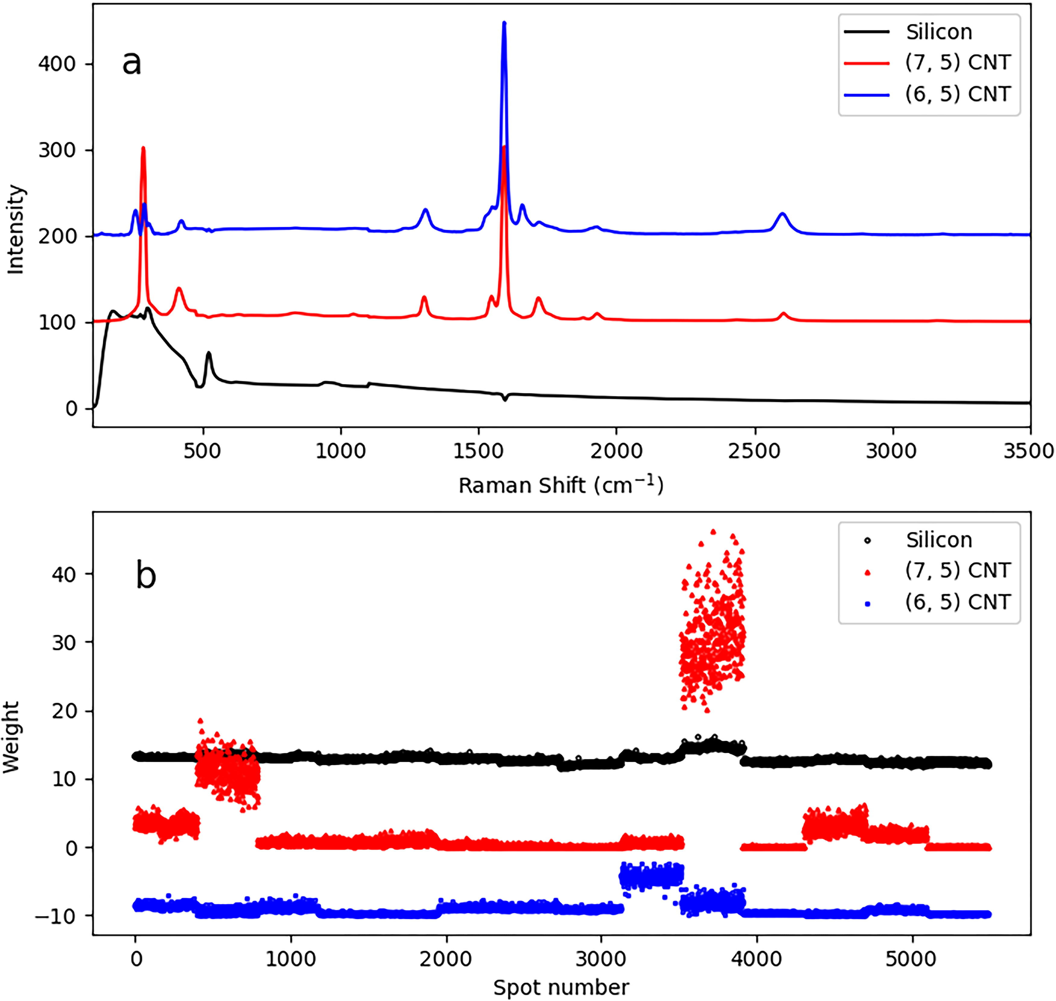
Deriving components and weights from all points and all samples. (a) Components obtained from all spots sampled for all dilution factors. Black, red, and blue (in sequence from bottom to top) are identified as components representing the silicon substrate background, (7,5) SWCNTs, and (6,5) SWCNTs, respectively. They have been offset vertically for clarity. (b) Corresponding weight of components at each spot. All spots on all samples are shown, each sample was measured at 400 spots. Each successive group of 400 points corresponds to a different sample from a different dilution. The bottom set, (6,5) blue, has been offset by −10 for clarity. The other two sets are not offset.

The choice of the number of components is a free parameter in the algorithm. In our case, we know a priori that the main components are the substrate, and the two pure SWCNT species matching the three components model. We explored the consequences of adding additional components (Figure S5, Supplemental Material). We found that choosing one extra component had a minor negative effect on our estimates of concentrations, which was significant only at low concentrations. When adding still more components, the algorithm tends to split real, physically interpretable features into parts with no clear physical meaning. So, it becomes challenging to relate the weight of the components to the concentration of any real species. Additionally, the software run time is usually shorter with fewer components. If, on the other hand, there are fewer components than species that are varying in reality, then the algorithm does not have enough free parameters to properly represent real variations in the data. Reducing components below three in our test case is problematic because there are at least three real contributions to the signal.

Unlike some other multivariate analysis techniques, there is not yet a generally accepted way to decide on the best number of components automatically from the data alone in NMF. However, statistical metrics which identify the best number of components are being developed and tested.^27–29 Given the progress in this area and its importance to practical applications, it seems likely that choosing the number of components will become an automated, standard part of NMF analysis in the near future.

Consistent data is essential for machine learning, and so the instruments gathering the data must be stable. We found that while NMF-derived spectral components seemed quite robust, the weights were very sensitive to focusing conditions. This can be understood because the depth of focus of the microscope objective was only ≈1 µm. We typically used 10 µm step sizes on a 20 × 20 step square grid, for a full scan range of 0.2 mm. Thus a ≈2 mrad tilt (≈0.1°) on the sample can go from perfect focus to outside of the focal depth over the lateral range of the scan.

To demonstrate, we exaggerated this effect by scanning a 10 × 10 grid with a 100 µm step size for a 1 mm wide scan range with a sample tilted by a few mrad (Figure 2). The NMF algorithm was set to search for five components (Figure 2a). This is more components than necessary, but the components are interpretable as SWCNT, silicon, or mixtures of both. However, all the measured weights vary widely and systematically (Figure 2b). This is purely an instrumental artifact, not a real physical variation of the distribution of SWCNTs on a sample. The weights are changing due to the sample drifting systematically out of focus.

Figure 2.

The importance of maintaining good focus. (a) Components extracted from a tilted sample. Five components were extracted. Components are offset by 20 arbitrary units for clarity. The middle component (green) is identified as purely SWCNTs while the other components contain SWCNT-like and silicon-like features. (b) Weight of each component at 90 spatial spots.

We solved this problem by using a tilt stage to adjust the angle of the sample. By moving a large distance (∼1 cm) laterally and adjusting the angle so both ends remained in good focus, we could essentially eliminate these variations on the millimeter scale. Alternatively, these effects can also be minimized by using a lower numerical aperture objective, so that the depth of focus is larger, or by restricting scans to a smaller distance scale. Either or both of these choices could be used by the operator to improve the usefulness of the data for analysis by the NMF algorithm.

Compared to silicon, the CaF₂ substrates were more challenging because they are transparent at visible wavelengths, and we used fairly low loadings of SWCNTs. Unless there is a strong signal from the surface it took more effort to find the right focus, and this led to large variations sample-to-sample or even on one sample. On silicon, the strong substrate peak, and lack of transparency makes focusing very easy. Furthermore, silicon substrates are available with exceptional flatness. The signal was also somewhat weaker on the CaF_2, but this is likely just because our deposition processes were developed for silicon, and it is likely that fewer SWCNTs were deposited. Because of the difficulty in confirming good focusing conditions, we do not explicitly show results from CaF₂, describing only silicon instead.

Next, we illustrate how data preprocessing improves concentration measurements by preventing convergence on spurious NMF components. For our samples, which are sparse (few SWCNTs ∼µm²) SWCNTs on SiO₂:Si, the raw spectra are dominated by the first order silicon peak at 520 cm⁻¹, with strong SWCNT peaks such as the G band around 1592 cm⁻¹ being an order of magnitude lower (Figures S2 and S3, Supplemental Material). When we used the raw data directly as the input to the NMF routine, we found that the components it pulled out were almost always weighted toward the most intense spectral feature: the first-order silicon peak. Perhaps unsurprising, this is just like the way that most people, when analyzing spectra or images, pay most attention to the brightest, strongest features. Furthermore, rather than pull out components that were related to SWCNTs, the NMF algorithm tended to split the silicon peak over multiple factors. This can be rationalized because a small relative change in a strong feature ends up being a large change in absolute mathematical terms. But those large changes were of little physical/chemical interest.

We found this problem could be managed simply by scaling down the intensity of the uninteresting silicon peak. Reducing this region by a factor of 10 made its intensity similar to the strongest SWCNT-related peaks. After this amount of scaling, the NMF-derived components matched well with the RS of the SWCNT species on the sample and led to a much better measure of the concentration.

Figure 3 shows the benefit of scaling. We specified that the algorithm should find three components. The components extracted from the unprocessed data are shown in Figure 3a. While usable, with one component clearly representing silicon and another clearly representing SWCNTs, the third component shows features of both. But after scaling the components become easily interpretable and we can identify the different SWCNT spectra with the two species of SWCNT, for example, based on the features in the RBM area. Figure 3b shows components extracted when the range 475–1100 cm⁻¹ was scaled down by a factor of 10, strongly reducing the influence of the silicon substrate background.

Figure 3.

The value of scaling down overpowering spectral features. (a) Components extracted directly. Black, red, and blue (bottom, middle, and top) are identified as silicon, SWCNTs, and a mixture of both. An offset has been applied for clarity. (b) Components extracted from scaled data. Black, red, and blue components (bottom, middle, and top) are identified as silicon, (7,5) SWCNTs, (6,5) SWCNTs, and are offset for clarity. (c) The relative weight of (7,5) SWCNTs for the unscaled (black, circle) and scaled (red, square) components as a function of the concentration. Error bars are the standard deviation from 400 spots. The black solid line is a linear best fit for the unscaled data with a slope of 0.40 ± 0.02 and an intercept of 0.04 ± 0.02 where the uncertainties are standard errors. The red dashed line is a linear best fit for scaled data with a slope of 0.419 ± 0.006 and an intercept of 0.005 ± 0.005. The gray dotted line shows where the relative weight equals the dilution factor, matching them at the highest concentration. The arrows indicate the weight returned for a bare silicon sample for unscaled (black, lower) and scaled (red, higher) data (i.e., blank concentrations).

This scaling makes the NMF weights follow the solution concentration down by over an order of magnitude more than the unprocessed data (Figure 3c). The arrows in Figure 3c show the weight given to SWCNT-like components for silicon samples with no SWCNTs, and so represent a concentration that is a “limit of blank.” The scaled data goes right down to this limit, while the unscaled data does not.

Weighting like this is a simple ad hoc solution to the challenges of our particular data sets. However, this sort of problem is a well-recognized challenge. There are algorithms that extend NMF to deal specifically with the need to de-emphasize uninteresting components and/or to try to better bring out weak contribution.^30,31, for example, the weighted NMF algorithm allows a weight to be attached to each feature.^32,33 So, there are promising approaches beyond the simple treatment we used here.

The NMF algorithm has to find both the components and the weights. So, it is interesting to compare its estimate of concentration to what would be obtained from the much simpler problem of having known components and making linear combinations to derive the weights. Figure 4a shows the pure spectra of the substrates, and the (7,5) and (6,5) SWCNT species separately. The pure SWCNT components have been constructed by taking a spectrum of SWCNTs on the substrate and subtracting a spectrum taken from the bare substrate. There is a good correspondence between these and the NMF components shown in Figure 4b. The silicon peak region normalization procedure has been used, scaling the intensity in the silicon peak region down by a factor of 10.

Figure 4.

Components and relative weights from linear combinations compared to those from the algorithm. (a) Spectra of pure samples. Black, red, and blue (bottom, middle, and top) are identified as silicon, (7,5), and (6,5) SWCNTs, respectively. An offset has been applied for clarity. (b) Components from NMF. The same color scheme is used. (c) The relative weight of (7,5) SWCNTs plotted as a function of concentration. Black (circles): linear combination of pure spectra. Red (squares): NMF. The error bars are the standard deviation for a sample of 400 spots. The black solid line is a linear best fit for the linear combination with a slope of 0.38 ± 0.01 and an intercept of 0.002 ± 0.003, where the uncertainties are standard errors. The red dashed line is a linear best fit for NMF with a slope of 0.394 ± 0.009 and an intercept of 0.006 ± 0.003. The gray dotted line shows where the relative concentration equals the dilution factor, matching them up at the highest concentration. The arrows indicate the weight for a bare substrate (i.e., the limit of blank) for the linear combination (black, lower) and NMF (red, upper).

Figure 4c compares the derived (7,5) species weights to the experimental solution concentrations. The mean weight over all the points on the sample is plotted with the error bars being the standard deviation. The relative weight is plotted, meaning all the weights are normalized so that the highest weight is 1. This relative weight tracks the concentration very well over almost three orders of magnitude. The uncertainty becomes large for relative weights of order 10⁻³, but the linear combination of known spectra goes deeper and appears to remain close to expected values down to a few parts in 10⁻⁴. The solid black line and dashed red line fit the data on a linear scale.

A better fit would be obtained with more free parameters than a linear fit which may be overly biased by high concentrations data. At very low concentrations the data points track well right down to the “limit of blank” concentration, that is, the concentration that was output for the bare substrate without SWCNTs. A quadratic or higher polynomial will model the data better over this large range of concentrations. The NMF-derived concentration is meaningful down to absolute concentrations of the source liquid dispersion in the few 10⁻³ mg/L, which corresponds to relative concentrations (compared to the highest concentration pure dispersions) of a few parts per thousand (ppt). A linear combination of known spectra gets into the 10⁻³ mg/L concentration range, corresponding to the mid-100 parts per million (ppm) range of relative concentrations.

The duration of the measurement is a practical issue, and that scales linearly with the number of spots that are sampled. To evaluate how many points are needed, we averaged over different numbers of points (Figure S6, Supplemental Material). A very small number of points gave quite a good estimate of relative weight for high concentrations and even a somewhat indicative estimate at low concentrations. However, if a precise estimate of the concentration is needed anywhere in dilution ranges from 10% to ppt level, samples of about 100 points are needed to bring the statistical scatter down to an acceptable level. Of course, this will depend on how sparsely, homogeneously, and randomly material is distributed on the substrate.

The RS from SWCNT is resonant, and this can be exploited for trace detection and concentration measurement. Above we used a 633 nm laser which is strongly resonant with the (7,5) nanotube. If we choose an excitation wavelength for which one analyte is resonant and the other is not, we can determine the concentration of that resonant analyte over a range of three orders of magnitude independent of the non-resonant analyte. If we then choose another wavelength for which only the other analyte is resonant, we can track its concentration over a similar range. Thus, by measuring two wavelengths, and determining two concentrations separately, we in principle measure the abundance of one analyte compared to the other over a dynamic range corresponding to six orders of magnitude.

There is, however, a fundamental consideration. Resonance is not binary: it is not switched on and then switched off. In reality, every Raman band has its own resonance window, with its own range of excitation wavelengths.^34,35 This is in part because there are two separate resonances, one corresponding to RS on resonance with the incoming phonon, and one corresponding to the outgoing phonon. Also, multiple-phonon scattering and the shape of the real electronic/excitonic density of states, which is more complicated than one single level, make the resonance window broad, (i.e., covering more laser wavelengths) and give it more structure.

The resonant windows are wider the higher energy the phonon mode is, and the width of the window, in energy units, e.g., eV, is comparable to the energy of the phonon mode. Although 561 nm is resonant with (6,5) and 633 nm is resonant with (7,5), these wavelengths are only 251 meV apart. The 2D band is at 2700 cm⁻¹ corresponds to 334 meV. So, the 2D band resonance for the (7,5) SWCNT may be strong at much shorter wavelengths than its excitonic resonance near 633 nm.

We experimented with independently measuring the (6,5) concentration with a 561 nm laser, for which the (6,5) SWCNT is somewhat resonant. Unfortunately, the dichroic beamsplitter that we used was not ideal as its transition region was at about 400 cm⁻¹, and so the otherwise prominent RBM peak of the (6,5) was dramatically reduced in intensity. This is not a fundamental issue, just a weakness of our current setup.

At 633 nm, there were many strong SWCNT peaks from the pure (7,5) SWCNT sample (Figure S2, Supplemental Material) as expected, given this is close to the E₂₂ resonance. There was a very weak but detectable SWCNT signal from the (6,5) SWCNT for bands above 1500 cm⁻¹. At 561 nm, there were many strong SWCNT peaks for the (6,5) SWCNT sample (Figure S3, Supplemental Material). The SWCNT signal from the (7,5) SWCNT sample signal was very weak, except for the 2D band which was still quite strong. This is consistent with the resonant window picture described above.

Figure 5 shows how the choice of laser wavelength affected the estimation of concentration. Figure 5a shows three components from NMF for data obtained by scanning at 633 nm. A silicon substrate component and components that are interpretable as (7,5) and (6,5) SWCNTs are obtained. Figure 5b shows three components from 561 nm. A substrate component and component interpretable as (6,5) SWCNTs is obtained, as well as a component that has very weak features except for the high wavenumber range. This peak matches well with the (7,5) SWCNT 2D band (2607 cm⁻¹).

Figure 5.

Components and relative weights derived from different laser wavelengths. (a) Components determined using a laser at 633 nm Black, red, and blue (bottom, middle, top) are identified as silicon, (7,5), and (6,5) SWCNTs, respectively. An offset has been applied for clarity. (b) Components determined using a laser at 561 nm. The same color scheme is used. (c) Weights of the (7,5)-like components as a function of the dilution factor. The weights are determined for each laser wavelength: 633 nm (red circles) and 561 nm (yellow squares). The error bars are the standard deviation for 400 spots. The red solid line is a linear best fit for 633 nm with a slope of 0.419 ± 0.006 and an intercept of 0.005 ± 0.005 where the uncertainties are standard errors. The yellow dashed line is a linear best fit for 561 nm with a slope of 0.41 ± 0.02 and an intercept of 0.04 ± 0.02. The gray dotted line shows where the relative concentration matches the dilution factor, based on matching the highest concentration. The red (top) and yellow (bottom) arrows show the concentration derived from the bare substrate (i.e., “limit of blank”) for the 633 nm and 561 nm laser, respectively.

The relative weight, taken from the mean weight (error bars are the standard deviation) is shown in Figure 5c, plotted as a function of (7,5) concentration. The relative weight derived from the 633 nm (7,5) component is plotted as red dots, with the error bars being standard deviation. The solid red line is a simple linear fit to the data. As before, relative weights can be tracked over almost three orders of magnitude, right down to the silicon substrate “limit of blank” shown as a red arrow.

In Figure 5, the yellow squares plot the mean weights of the 561 nm derived 2D band-dominated component. It tracks the relative concentration of the (7,5) from the 633 nm laser data down to the few percent relative weight level, corresponding to initial liquid dispersions at 10⁻²mg/L to 10⁻¹ mg/L. In this way, the “wrong wavelength” can be used to track concentrations in resonant RS.

This is also a kind of “crosstalk” that could limit the range of the ratios of the two species that we can measure. Consider the simplified model that the resonance window starts at the absorption resonance and runs exactly to the absorption resonance plus the phonon energy.³⁴ For the (7,5) nanotube, the nominal absorption resonance (“E₂₂”) is at 645 nm.²³ The 561 nm laser is at dE = 2321 cm⁻¹ higher in energy than E₂₂. So, in this model, for the (7,5) species any Raman mode with energy above dE will still be resonant at 561 nm, e.g., the 2D band (∼2600 cm⁻¹). However, any Raman mode below dE will not be resonant and so will be very weak for the 561 nm laser, e.g., the G band (∼1590 cm⁻¹). These lower energy modes will be resonant for a laser closer to E_22, though (e.g., 633 nm). If the mode frequencies and line shapes do not change much with chirality and they are high energy (≥dE), they will be resonant for both lasers and hard to separate. Crosstalk is a problem then. However, if they are lower in energy (<dE), they will be separately visible at the different laser wavelengths, and it will be easy to track each species separately—there will be no problem with crosstalk. The different species will be easy to distinguish, even if their Raman spectral features are similar in frequency and line shape.

So here, if we want to use the 561 nm laser to measure trace (6,5) SWCNTs in a predominantly (7,5) ensemble, it is most effective to use only the smaller Raman shifts (less than dE).

Conclusion

We have used Sci-kit Learn's implementation of the NMF algorithm to automate the detection and determination of the concentration of chirally pure SWCNTs from spatially scanned hyperspectral RS data. For a series of samples, a practical and effective procedure is to batch all samples at all concentrations together and pull out only one set of components for the entire set. Then the weight of each component scales with concentration. We identified and documented several practical considerations when making such measurements. The NMF outputted weights, which determine the concentration, are sensitive to focusing conditions. By taking simple precautions, variability due to these effects can be eliminated. The NMF algorithm itself, as-is, is biased toward strong spectral features. This bias can be overcome by normalizing uninteresting but overly intense features. The NMF algorithm, with no a priori input of spectral components, comes close to estimating the concentration as well as a linear combination based on a full knowledge of the spectra (i.e., from a spectral library).

Using an order of 100 spatial points, with one laser wavelength, µg/L measurements are obtained, corresponding to the ppt relative concentration level. Choosing two different laser wavelengths resonant with two different species each separately and independently having ppt ranges of three orders of magnitude provides a dynamic range in the concentration of one species versus the other of up to six orders of magnitude. However, the laser wavelengths should be separated in energy by at least the Raman shift energy of the phonon mode to prevent crosstalk. Concentration measurements can be obtained even with the “wrong” laser if peaks at large Raman shifts are used.

Open-source software is already valuable for the application of multivariate data analysis/machine learning to chemical analysis, and it is likely to grow in importance. From a metrology perspective, open-source software is important because it makes it possible for essentially anyone to check the analysis.

There are easy opportunities to move this toward higher purity levels. The coverage of the majority species can be made much higher, for example, and should have little impact on the minority signal as long as the spacing between laser resonances is large enough in energy. Coverage could be increased with longer depositions, repeated depositions, or starting with more concentrated dispersions (>few mg/L). There are also opportunities to improve the usefulness of the algorithm, for example, to automate the choice of the number of features, and to refine normalization procedures to be best suited to analytical goals such as trace contaminant detection or precision quantification of a known species.

Finally, Raman spectra are ordinarily one-dimensional data sets, multi-dimensional resonant Raman data where each spectrum is a 2D image are also being explored.^34,35 Although sure to be more computationally demanding, since NMF is useful for image analysis,¹³ we expect it will also be well suited to that higher dimensional type of hyperspectroscopy.

Supplemental Material

sj-docx-1-app-10.1177_27551857241281755 - Supplemental material for Automating Trace Detection and Chemical Purity Analysis of Carbon Nanotube Mixtures by Non-Negative Matrix Factorization of Spatial Raman Scattering Hyperspectra

Supplemental material, sj-docx-1-app-10.1177_27551857241281755 for Automating Trace Detection and Chemical Purity Analysis of Carbon Nanotube Mixtures by Non-Negative Matrix Factorization of Spatial Raman Scattering Hyperspectra by Justin X. Wong, Jianying Ouyang, François Lapointe, Brendan Mirka and Paul Finnie in Applied Spectroscopy Practica

Footnotes

Acknowledgment

We are grateful to Simona Moisa for the technical support with the atomic force microscope.

Declaration of Conflicting Interests

The authors declared no potential conflicts of interest with respect to the research, authorship, and/or publication of this article.

Funding

The authors received no financial support for the research, authorship, and/or publication of this article.

ORCID iDs

Justin X. Wong

François Lapointe

Brendan Mirka

Paul Finnie

Supplemental Material

All supplemental material mentioned in the text is available in the online version of the journal.

References

Wei

Flavel

Krupke

Chen

. “Exploring the Upper Limit of Single-Walled Carbon Nanotube Purity by Multiple-Cycle Aqueous Two-Phase Separation”. Nanoscale. 2017. 9(32): 11640‐11646. https://doi.org/10.1039/c7nr03302h

Yang

Wang

Zhang

Yang

, et al. “Chirality Pure Carbon Nanotubes: Growth, Sorting, and Characterization”. Chem. Rev. 2020. 120(5): 2693‐2758. https://doi.org/10.1021/acs.chemrev.9b00835

Tulevski

Franklin

Frank

Lobez

, et al. “Toward High-Performance Digital Logic Technology with Carbon Nanotubes”. ACS Nano. 2014. 8(9): 8730‐8745. https://doi.org/10.1021/nn503627h

Chen

Dasgupta

Morrow

Emmanuele

, et al. “Room Temperature Lasing from Semi-Conducting Single-Walled Carbon Nanotubes”. ACS Nano. 2022. 16(10): 16776‐16783. https://doi.org/10.1021/acsnano.2c06419

Htoon

Doorn

S.K.

Pernice

W.H.P.

, et al. “Carbon Nanotubes as Emerging Quantum-Light Sources”. Nature Mater. 2018. 17(8): 663‐670. https://doi.org/10.1038/s41563-018-0109-2

Ackermann

Metternich

J.T.

Herbertz

Kruss

. “Biosensing with Fluorescent Carbon Nanotubes”. Ang. Chem. 2022. 61(8): e202112372. https://doi.org/10.1002/anie.202112372

McCreery

R.L.

. Raman Spectroscopy for Chemical Analysis. New York: John Wiley and Sons, 2000. Pp. 410.

Jorio

Saito

. “Raman Spectroscopy for Carbon Nanotube Applications”. J. Appl. Phys. 2021. 129(2): 021102. https://doi.org/10.1063/5.0030809

Lefebvre

Finnie

Fagan

J.A.

Zheng

Hight Walker

A.R.

. “Metrological Assessment of Single-Wall Carbon Nanotube Materials by Optical Methods”. In: Weisman

R.B.

Kono

, editors. Handbook of Carbon Nanomaterials. New Jersey: World Scientific, 2019. Vols. 9 and 10. Chap. 2, Pp. 45‐104. https://doi.org/10.1142/10862

10.

Finnie

Ding

Kingston

C.T.

. “Assessment of the Metallicity of Single-Wall Carbon Nanotube Ensembles at High Purities”. J. Phys. Chem. C. 2014. 118(51): 30127‐30138. https://doi.org/10.1021/jp506945f

11.

Ding

Finnie

Lefebvre

, et al. “Raman Microscopy Mapping for the Purity Assessment of Chirality Enriched Carbon Nanotube Networks in Thin-Film Transistors”. Nano Res. 2015. 8(7): 2179‐2187. https://doi.org/10.1007/s12274-015-0725-y

12.

Berry

M.W.

Browne

Langville

A.N.

Pauca

V.P.

Plemmons

R.J.

. “Algorithms and Applications for Approximate Nonnegative Matrix Factorization”. Comput. Stat. Data Anal. 2007. 52(1): 155‐173. https://doi.org/10.1016/j.csda.2006.11.006

13.

Lee

D.D.

Seung

H.S.

. “Learning the Parts of Objects by Nonnegative Matrix Factorization”. Nature. 1999. 401(6755): 788‐791. https://doi.org/10.1038/44565

14.

Adal

Wang

Emge

Cichocki

. “Non-Negative Matrix Factorization with Orthogonality Constraints and its Application to Raman Spectroscopy”. J. VLSI Signal Process. Syst. Signal Image Video Technol. 2007. 48: 83‐97. https://doi.org/10.1007/s11265-006-0039-0

15.

Pedregosa

Varoquaux

Gramfort

Michel

, et al. “Scikit-Learn: Machine Learning in Python”. J. Mach. Learn. Res. 2011. 12: 2825‐2830. https://doi.org/10.5555/1953048.2078195

16.

Ntziouni

Thomson

Xiarchos

, et al. “Review of Existing Standards, Guides, and Practices for Raman Spectroscopy”. Appl. Spectrosc. 2022. 76(7): 747‐772. https://doi.org/10.1177/00037028221090988

17.

Barton

Thomson

Diz

Portela

. “Chemometrics for Raman Spectroscopy Harmonization”. Appl. Spectrosc. 2022. 76(9): 1021‐1041. https://doi.org/10.1177/00037028221094070

18.

Flores

Ouyang

Lapointe

Finnie

. “Nanotube Abundance from Non-Negative Matrix Factorization of Raman Spectra as an Example of Chemical Purity from Open Source Machine Learning”. Sci. Rep. 2022. 12(1): 11666. https://doi.org/10.1038/s41598-022-15359-4

19.

Ozawa

Ide

Fujigaya

Niidome

Nakashima

. “One-Pot Separation of Highly Enriched (6,5)-Single-Walled Carbon Nanotubes Using a Fluorene-Based Copolymer”. Chem. Lett. 2011. 40(3): 239‐241. https://doi.org/10.1246/cl.2011.239

20.

Ouyang

Ding

Lefebvre

. “Sorting of Semiconducting Single-Walled Carbon Nanotubes in Polar Solvents with an Amphiphilic Conjugated Polymer Provides General Guidelines for Enrichment”. ACS Nano. 2018. 12(2): 1910‐1919. https://doi.org/10.1021/acsnano.7b08818

21.

Ouyang

Shin

Finnie

Ding

. “Impact of Conjugated Polymer Characteristics on the Enrichment of Single-Chirality Single-Walled Carbon Nanotubes”. ACS Appl. Polymer Mat. 2022. 4(8): 6239‐6254. https://doi.org/10.1021/acsapm.2c01022

22.

Streit

J.K.

Bachilo

S.M.

Ghosh

Lin

C.-W.

Weisman

. “Directly Measured Optical Absorption Cross Sections for Structure-Selected Single-Walled Carbon Nanotubes”. Nano Lett. 2014. 14(3): 1530‐1536. https://doi.org/10.1021/nl404791y

23.

Weisman

R.B.

Bachilo

S.M.

. “Dependence of Optical Transition Energies on Structure for Single-Walled Carbon Nanotubes in Aqueous Suspension: An Empirical Kataura Plot”. Nano Lett. 2003. 3(9): 1235‐1238. https://doi.org/10.1021/nl034428i

24.

Lefebvre

Finnie

. “Excited Excitonic States in Single-Walled Carbon Nanotubes”. Nano Lett. 2008. 8(7): 1890‐1895. https://doi.org/10.1021/nl080518h

25.

Itoh

Shirono

. “Reliable Estimation of Raman Shift and its Uncertainty for a Non-Doped Si Substrate (NMIJ CRM 5606-a)”. J. Raman Spectrosc. 2020. 51(12): 2496‐2504. https://doi.org/10.1002/jrs.6003

26.

Jorio

Dresselhaus

Saito

Dresselhaus

. Raman Spectroscopy in Graphene Related Systems. Weinheim, Germany: Wiley-VCH, 2011.

27.

Schulze

H.G.

Konorov

S.O.

Piret

J.M.

Blades

M.W.

Turner

R.F.B.

. “Empirical Factors Affecting the Quality of Non-Negative Matrix Factorization of Mammalian Cell Raman Spectra”. Appl. Spectrosc. 2017. 71(12): 2681‐2691. https://doi.org/10.1177/0003702817732117

28.

Maisog

J.M.

DeMarco

A.T.

Devarajan

Young

S.S.

, et al. “Assessing Methods for Evaluating the Number of Components in Non-Negative Matrix Factorization”. Mathematics. 2021. 9(22): 2840. https://doi.org/10.3390%2Fmath9222840

29.

Cai

Kenney

. “Rank Selection for Non-Negative Matrix Factorization”. Stat. Med. 2023. 42(30): 5676‐5693. https://doi.org/10.1002/sim.9934

30.

Chen

Gong

. “Feature Weighted Non-Negative Matrix Factorization”. IEEE Trans. Cybern. 2023. 53(2): 1093‐1105. https://doi.org/10.1109/TCYB.2021.3100067

31.

Wang

Liu

. “Cluster-Wise Weighted NMF for Hyperspectral Images Unmiing with Imbalanced Data”. Remote Sens. 2021. 13(2): 1‐19. https://doi.org/10.3390/rs13020268

32.

Blondel

V.D.

N.-D.

van Dooren

. “Weighted Nonnegative Matrix Factorization and Face Feature Extraction”. https://perso.uclouvain.be/paul.vandooren/publications/BlondelHV07.pdf [accessed August 23 2024].

33.

Blondel

N.-D.

van Dooren

. “wNMF: Weighted Non-Negative Matrix Factorization”. https://github.com/asn32/weighted-nmf [accessed September 13 2024].

34.

Finnie

Ouyang

Fagan

J.A.

. “Broadband Full-Spectrum Raman Excitation Mapping Reveals Intricate Optoelectronic–Vibrational Resonance Structure of Chirality-Pure Single-Walled Carbon Nanotubes”. ACS Nano. 2023. 17(8): 7285-7295. 10.1021/acsnano.2c10524

35.

Finnie

Ouyang

Lefebvre

. “Full Spectrum Raman Excitation Mapping Spectroscopy”. Sci. Rep. 2020. 10(1): 9172. https://doi.org/10.1038/s41598-020-65757-9

Supplementary Material

Please find the following supplemental material available below.

For Open Access articles published under a Creative Commons License, all supplemental material carries the same license as the article it is associated with.

For non-Open Access articles published, all supplemental material carries a non-exclusive license, and permission requests for re-use of supplemental material or any part of supplemental material shall be sent directly to the copyright owner as specified in the copyright notice associated with the article.

0.00 MB

1.32 MB