Sage Journals: Discover world-class research

Abstract

New stations (such as metro stations) will bring remarkable changes to the local transportation and economic development. Understanding patterns of factors which importantly impact on public transit ridership in the surrounding areas of new stations is essential to their construction planning, like estimating the possible ridership. Built environment variables with high importance magnitude, which were thought applicable to estimate public transit ridership in other areas of the same category, were described as transferable variables (TVs) in this study. A transferability analysis method of the built environment for the ridership estimation was constructed by adopting partial least square regression (PLSR) based on available data. Taking Wuhan, China as an example, this study analyzed the changes and differences of the built environment variables in different categories of pedestrian catchment areas (PCAs) of metro stations on the importance and transferability magnitude for the metro and taxi ridership, based on the metro and taxi data of one week in January, April, and June. Performances of the ridership estimation based on TVs and all the built environment variables were compared. This study inferred that (1) most of the land use variables (about 85%) showed important influence on the metro and taxi ridership, while only about 18% of the other variables showed key impact. The importance magnitude of the built environment variables was mainly related to PCA categories and public transportation modes, but less related to time. (2) Highly important built environment variables also tended to be highly transferable. Transferability magnitude of the built environment variables for the ridership was related to PCA categories and types of public transport. (3) Compared to all the built environment variables, using TVs, the relative accuracy of the metro and taxi ridership estimation was around 20% and 18% higher respectively.

Keywords

Transit ridership built environment partial least squares regression relative importance transferable variables

Highlights

Exploring the public transit ridership (metro and taxi) in different categories of pedestrian catchment areas of metro stations in Wuhan.

Understanding the importance and transferability magnitude of the built environment variables for the metro and taxi ridership estimation.

Comparing the ridership estimation results based on transferable variables and all the built environment variables.

The findings could be helpful in the decision-making process for constructing new metro stations.

Introduction

The built environment in the pedestrian catchment areas (PCAs) of metro, train, or bus stations plays an important role in attracting human activities (Yang et al., 2016), which have a significant influence on the public transit ridership within it (Chakour and Eluru, 2016). The estimation of public transit ridership is a critical task for the planning of new stations. Their construction is expensive and difficult to abandon or replace. New stations bring significant changes to the traffic situation and the development of the surrounding areas. However, there are no existing public transit ridership data in such new areas. Therefore, based on the accessible data, this study attempts to use the built environment variables in the PCAs of existing stations to estimate the ridership in those of new stations. This study is significant for the scientific planning and operation of urban public transportation systems.

Many models have been proposed to determine the relationship between the built environment variables and public transit ridership and estimate the ridership. For example, (1) the four-step model, which considers trip generation, distribution, mode choice, and route assignment for modeling and estimating ridership, has been used by scholars worldwide (McNally, 2007). However, Marshall and Grady (2006) pointed such a model would invite several potential problems, such as model accuracy, sensitivity to land use, institutional barriers, and cost of use. (2) The activity-based model assumes that traveling is the derivation of the demand for personal activities (Shiftan and Suhrbier, 2002). Although this model can estimate ridership by generating time- and mode-specific trip matrices, it is expensive to implement and maintain (Bowman and Ben-Akiva, 2001). Zhao et al. (2014b) pointed out that transit providers usually would not be able to participate in modeling and estimation, which would restrict quick response to the results. (3) Direct ridership models (DRMs), which overcome the disadvantages of the four-step and activity-based models, have recently gained significant attention (Kepaptsoglou et al., 2017). DRMs based on regression analysis are complementary approaches for estimating ridership as a function of the built environment and transit service features within the surroundings of stations (Cervero, 2006; Chu, 2004; Gutiérrez et al., 2011; Kuby et al., 2004). Compared to the above two models, DRMs have faster responses and lower costs, and are simpler to apply, validate, and develop (Cardozo et al., 2012; Walters and Cervero, 2003). Additionally, DRMs results are easier to analyze and explain, which may enable one to precisely understand the impact of built environment variables on public transit ridership (Gutiérrez et al., 2011). Generally, the ridership and built environment are always taken as dependent and independent variables, respectively. The impact of the built environment variables on the ridership at different times (weekdays, weekends, peak, and non-peak periods) is determined through a particular model and measured by the corresponding variable coefficients. The values of the coefficients reflect the impact magnitude of independent variables on dependent variables, and the sign determines the correlation (positive or negative correlation) between the two.

With the accessible data, this study took Wuhan, China as an example to understand the importance magnitude of the built environment on travel patterns of urban residents in more detail. In this study, built environment variables with high importance magnitude, which were thought suitable for ridership estimation in other areas of the same category, were defined as transferable variables (TVs). Transferability magnitude indicated the length of time when built environment variables were transferable or maintained high importance magnitude to transit ridership variables. The longer built environment variables were transferable, the higher transferability magnitude they had. Partial least square regression (PLSR) was adopted to explore the importance magnitude of each built environment variable, which was represented by the variable importance in project (VIP) values, for the metro and taxi ridership in different categories of PCAs of metro stations. Besides, this study further analyzed the transferability magnitude with time and evaluated the estimation performance with TVs. This study helps to optimize the regional industrial layout and traffic planning to meet the dynamic changes in the travel needs of urban residents, as well as providing a scientific base for the construction and development of the same category of metro stations based on the available data.

The remainder of this paper was organized as follows. The existing literature was reviewed in section “Literature review”. The study area and dataset used were described in section “Study area and data”. The study process was described in section “Methods”. In section “Result and discussion”, the importance and transferability magnitude of the built environment for metro and taxi ridership were analyzed, and ridership estimation was evaluated. Finally, section “Conclusion” summarized the study and discusses its disadvantages as well as future scope.

Literature review

Modeling and estimating public transit ridership is essential for analyzing the project viability of stations and the development of urban areas (Zhao et al., 2013). There are three main categories of DRMs: traditional, spatial (Guo and Huang, 2020), and machine learning models. In the traditional category, ordinary least squares (OLS) regression is considered as the basic approach (An et al., 2019; Kim et al., 2016; Sohn and Shim, 2010; Zhao et al., 2013). Other types of models in this category include Poisson regression (Chu, 2004), negative binomial regression (Thompson et al., 2012), stepwise regression (Currie et al., 2011; Li et al., 2020), and PLSR (Chen et al., 2022; Zhao et al., 2014a). Furthermore, some studies have estimated the ridership from multiplicative models (Choi et al., 2012; Zhao et al., 2014b). These are estimated to be linear models following logarithmic transformation, and hypothesize that the ridership is associated with the product of explanatory factors (Kepaptsoglou et al., 2017).

Many scholars adopt spatial models to take spatial effects into consideration. Geographically weighted regression (GWR) has been implemented in empirical studies in many economically developed areas with high population density, such as Sydney (Blainey and Mulley, 2013), New York City (Qian and Ukkusuri, 2015), Seoul (Sung et al., 2014), and Beijing (Zhu et al., 2019). Besides, in order to overcome the GWR limitations, improved versions of GWR, like multi-scale geographically weighted regression (MGWR) (Fotheringham et al., 2017) and geographically and temporally weighted regression (GTWR) (Fotheringham et al., 2015) have been proposed and adopted. For example, Lyu et al. (2020) explored the multi-scale spatial relationship between public bicycle ridership and built environment in Nanjing. Ma et al. (2018) applied GTWR to investigate the spatiotemporal influence of the built environment on the hourly public transit ridership in Beijing. Additionally, other types of spatial models, such as distance-decay weighted regression (Gutiérrez et al., 2011) and network kriging regression (Zhang and Wang, 2014), have been implemented.

Nowadays, although linear and log-linear regression methods have been the most prevalent models in this research area, some scholars begin to argue that it is also essential to discard the assumption that a linear relationship or log-linear relationship exists between these two research targets (Ding et al., 2019; Gan et al., 2020). Therefore, machine learning models have recently been taken prevalence and used gradually (Yan et al., 2020). Ding et al. (2019) employed gradient boosting decision trees to investigate the non-linear influence of the built environment on average weekday passenger boarding of metro stations. Additionally, Gan et al. (2020) adopted gradient boosting regression model to explore the relationship between built environment and metro ridership at station-to-station level and compared to traditional multiplicative model.

The public transit ridership variation in the PCAs of stations is associated with the station characteristics and its surrounding environment (Chen et al., 2019; Gutiérrez et al., 2011; Li et al., 2019, 2020). The attributes of a station mainly comprise the distance to the city center (Ding et al., 2019) and the connection characteristics within the transit network, such as whether it is a terminal or transfer station and its closeness and betweenness centrality (Cardozo et al., 2012; Sohn and Shim, 2010). Land use of the surrounding environment reflects different human activities, and hence contributes to various public transit ridership (Chakraborty and Mishra, 2013). The proportions of residential, commercial, business, government, and industrial areas or floor area are the most chosen variables in the land use category (Tu et al., 2018), along with land use mix (Ding et al., 2019; Lee et al., 2013). Besides, points of interest (POIs) are able to reveal more detailed land use characteristics, therefore their impact on transit ridership are paid more attention gradually (An et al., 2019; Chen et al., 2019; Li et al., 2019). Demographic and socio-economic information is used to understand the daily travel plan of residents; population density is used to represent the activity demand of people and socio-economic factors, such as employment and income, are also associated with city-wide travel (Jun et al., 2015; Qian and Ukkusuri, 2015; Tu et al., 2018). External road connectivity characteristics, such as road length, intersection density, and road density (Jun et al., 2015), and intermodal connection factors, such as the number of bus stops and bus lines (Ding et al., 2019; Lee et al., 2013; Zhao et al., 2013), are used to reflect the accessibility of the station.

There are several research gaps regarding modeling and estimating public transit ridership that need to be filled: (1) How does the importance magnitude of the built environment variables for public transit ridership, such as metro systems and taxis, change? (2) Which built environment variables are transferable? Judging the transferability magnitude involves determining the key factors influencing the ridership. (3) The effect of using TVs to estimate ridership. Comparing the improvement in accuracy will help understand the role played by TVs, thereby providing new perspectives for ridership estimation.

In order to fill these gaps, this study made some improvements. First, stations were divided into different categories according to their surrounding land use, instead of considering all of them as a category. Stations are in various functional areas of the city, thus the difference of the influence on the transit ridership of the same built environment variable in different location might be ignored if the stations are grouped into one category. Second, unlike most studies focusing on one type of transportation mode, this study explored the metro and taxi ridership. The relationship between the built environment and transit ridership were analyzed more comprehensively. Finally, importance magnitude of built environment variables was analyzed. Previous studies always used the model coefficients to reflect the relationship between the built environment and ridership variables. However, they could not accurately reveal the importance magnitude of various built environment variables, due to the unit of different built environment variables. In this study, PLSR was selected to explore the impact of built environment variables on transit ridership, because of its relatively good performance on multicollinearity, model interpretability, and calculation cost (Chen et al., 2022). It is more effective when the number of samples is similar to or less than that of the variables (Qiao et al., 2018), which is more suitable for this study due to the stations’ classification. Moreover, this model provides the VIP value to reflect variable importance magnitude. Besides, there is a commonly used threshold of the VIP value, which is 1, to indicate a variable have high importance magnitude (important) or low one (unimportant) (Ong et al., 2021).

Study area and data

Study area

Wuhan is the capital city of the Hubei Province and transportation hub of central China. By the end of 2017, the Wuhan metro system had carried a total of 927 million passengers. The average daily ridership reached 2.54 million, which accounted for 23.5% of the city’s public transportation ridership. By 2020, there were 10 metro lines in Wuhan (Lines 1–8, Line 11, and Line Yangluo), with a total operating mileage of 360 km, and ranking 1st in central China. The distribution of the Wuhan metro system was illustrated in Figure 1. The foundation for classifying metro stations into different categories (work, residential, etc.) (Figure 1) is discussed under ‘Categories of PCAs’. It is observed that most of metro stations are located within the third ring road of Wuhan, which is the main urban zone. Currently, to support the construction of key development regions and alleviate urban traffic congestion, Wuhan is vigorously building its urban metro system, thus increasing the demand for scientific subway planning.

Figure 1.

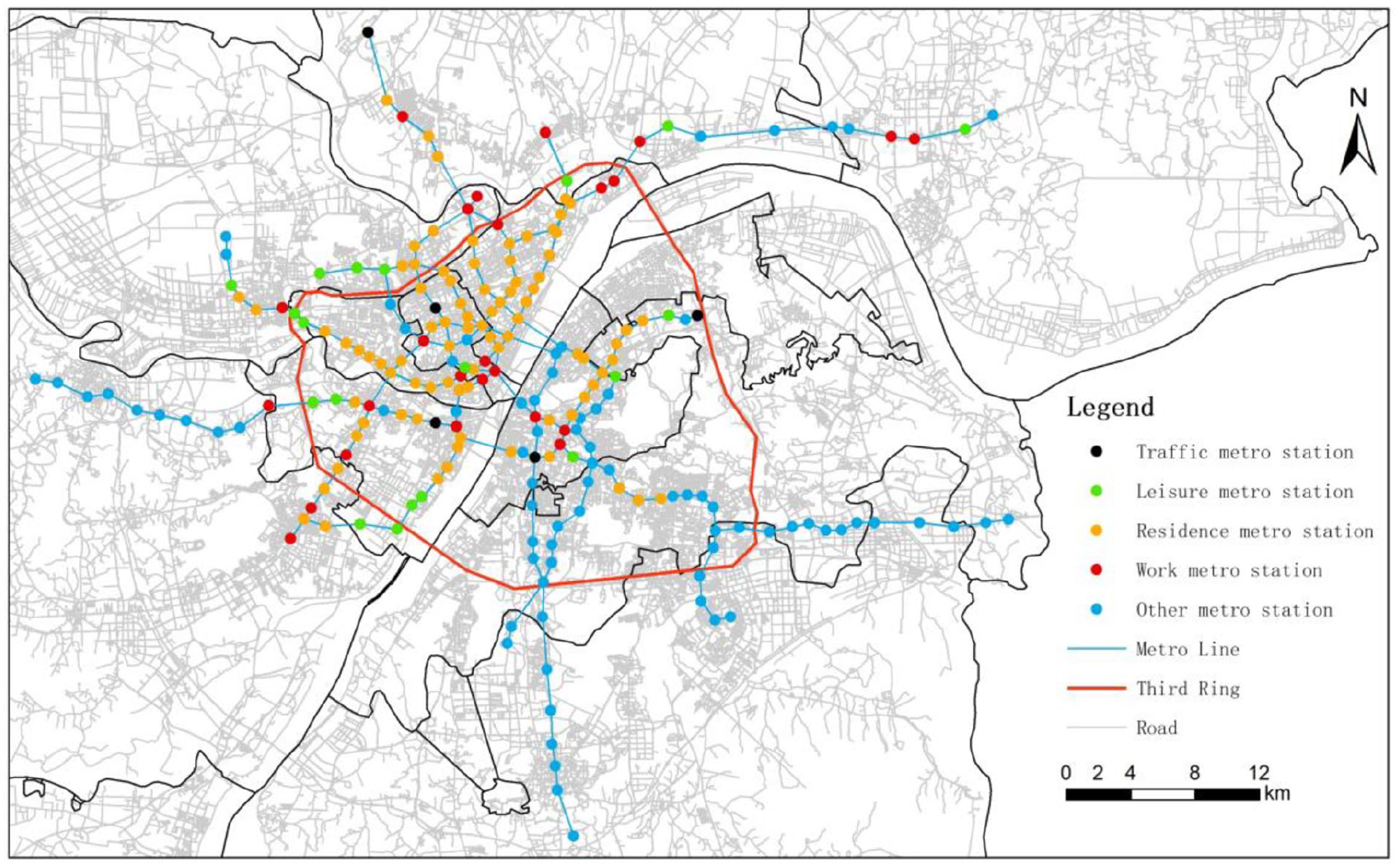
The Wuhan metro system.

Data description

Land planning, metro smart card (SCD), taxi GPS trajectory, POIs, roads, population distribution, and other city basic data were used in this study. Land planning data, obtained from the detailed city-wide regulatory plan, were used to classify PCAs. This legal plan provided specific guidance for the urban construction in Wuhan. Land planning data of Wuhan for 2020 enlisted 27 types of functional land, such as education and scientific research land. Metro SCD and taxi GPS trajectory data were used to calculate the flow of residents entering and leaving the PCAs through metro or taxi as the variables of public transit ridership. Metro SCD denoted the number of citizens traveling by metro in three weeks, namely 15–21 January, 16–22 April, and 4–10 June, 2018. Additionally, taxi GPS trajectory data revealed the operation of taxis during the same period. Road, POIs, population distribution, and other basic city data, such as bus stations, were described as the built environment variables in PCAs. The POIs from 2018 used in this study were collected by a web crawler using AMap APIs.

Methods

The research flow is illustrated in Figure 2. First, data were preprocessed to acquire metro and taxi ridership and built environment variables. Second, PCAs of metro stations were divided into different categories based on the main land planning types. Third, PLSR was adopted to model the built environment and public transit ridership (metro and taxi) in different categories of PCAs. Finally, the changes in the importance and transferability magnitude of the built environment variables for the ridership ones were analyzed, after which this study compared the differences in estimating ridership with TVs and all the built environment variables.

Figure 2.

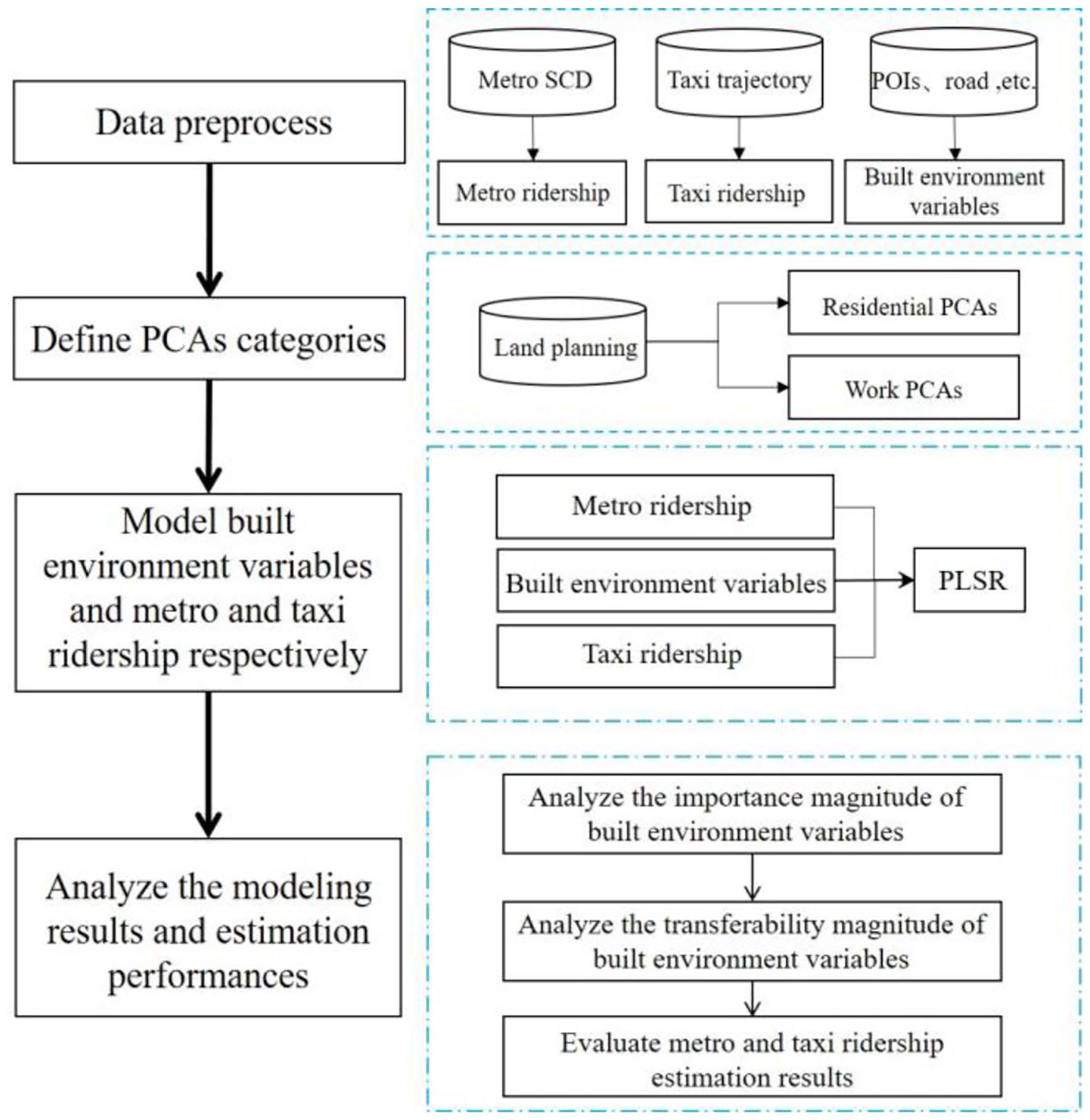
Research flow.

Categories of PCAs

Selection of the PCA range is essential in the studying the impact of the surrounding environment of metro stations on public transit ridership. The radius of PCAs is generally 300–900 m (Gan et al., 2020; Gutiérrez et al., 2011; Jun et al., 2015; Li et al., 2020). This study considered approximately 10 min walking time of residents as the threshold, so 600 m was chosen as the PCA radius. However, some PCAs overlapped when the straight-line distance between their corresponding metro stations was < 600 m. Therefore, the Thiessen polygons were adopted to intersect with the original PCAs to eliminate the overlap.

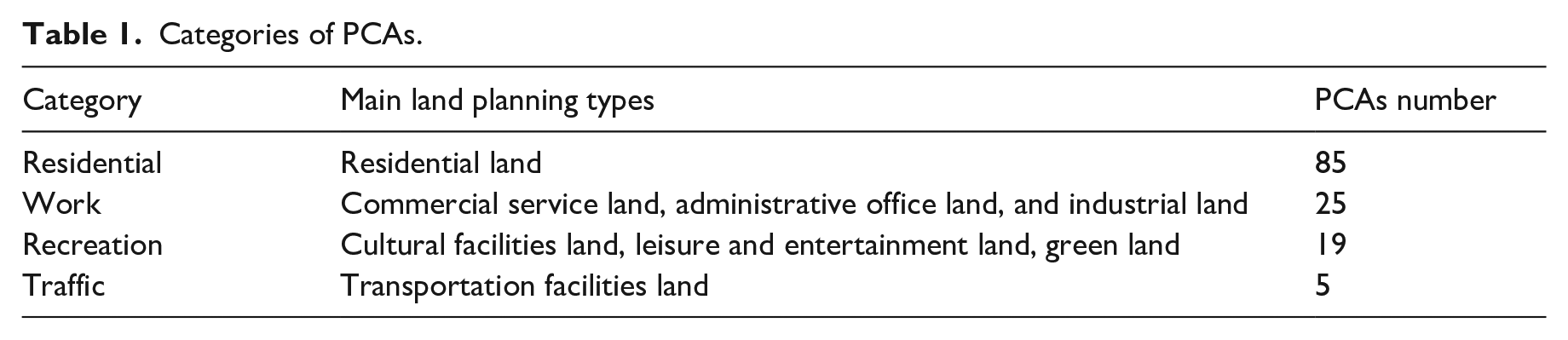
PCAs classification depended on The Athens Charter, which was developed by the Fourth Congress of the Congrès Internationaux d’Architecture Moderne (CIAM IV) in 1933. It is considered to be a programmatic document of modern urban planning and is an important reference for the planning and development of many cities (GOLD, 1998). There are four basic function categories of cities in The Athens Charter: residence, work, recreation, and transportation, according which the PCAs of this study were classified (Table 1). For example, PCAs mainly comprising commercial service, administrative office, and industrial land were classified under “work”. Due to limited number of PCAs, this study chose residential and work PCAs as the research objects.

Table 1.

Categories of PCAs.

Category	Main land planning types	PCAs number
Residential	Residential land	85
Work	Commercial service land, administrative office land, and industrial land	25
Recreation	Cultural facilities land, leisure and entertainment land, green land	19
Traffic	Transportation facilities land	5

Built environment and public transit ridership variables

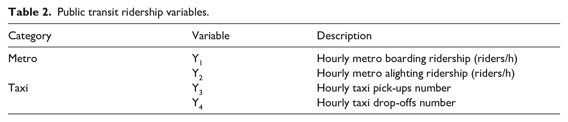
Public transit ridership and the built environment variables were set as dependent variables Y (Table 2) and independent variables X, respectively (Table 3).

Table 2.

Public transit ridership variables.

Category	Variable	Description
Metro	Y₁	Hourly metro boarding ridership (riders/h)
Metro	Y₂	Hourly metro alighting ridership (riders/h)
Taxi	Y₃	Hourly taxi pick-ups number
Taxi	Y₄	Hourly taxi drop-offs number

Table 3.

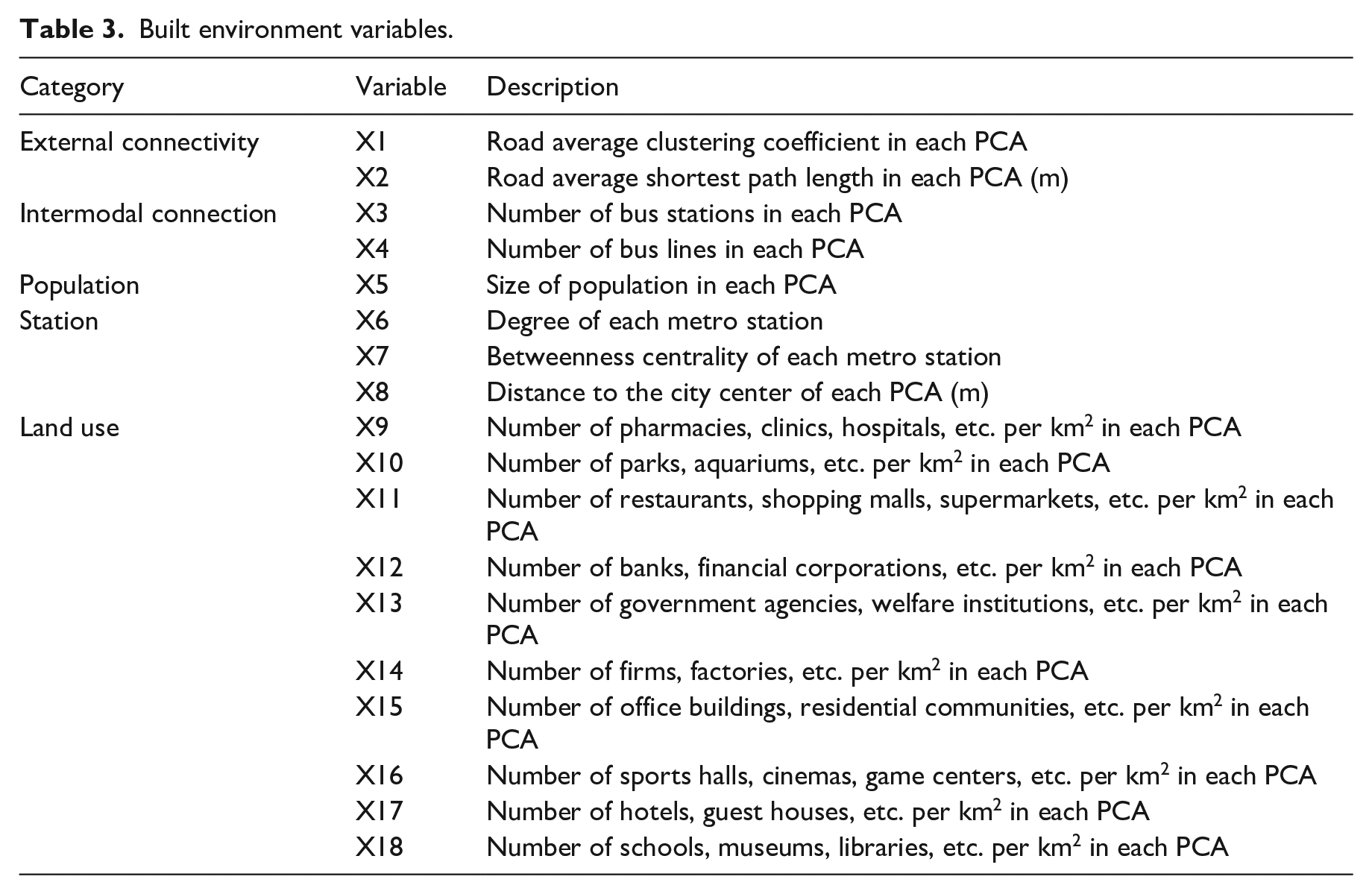
Built environment variables.

Category	Variable	Description
External connectivity	X1	Road average clustering coefficient in each PCA
External connectivity	X2	Road average shortest path length in each PCA (m)
Intermodal connection	X3	Number of bus stations in each PCA
Intermodal connection	X4	Number of bus lines in each PCA
Population	X5	Size of population in each PCA
Station	X6	Degree of each metro station
	X7	Betweenness centrality of each metro station
	X8	Distance to the city center of each PCA (m)
Land use	X9	Number of pharmacies, clinics, hospitals, etc. per km² in each PCA
	X10	Number of parks, aquariums, etc. per km² in each PCA
	X11	Number of restaurants, shopping malls, supermarkets, etc. per km² in each PCA
	X12	Number of banks, financial corporations, etc. per km² in each PCA
	X13	Number of government agencies, welfare institutions, etc. per km² in each PCA
	X14	Number of firms, factories, etc. per km² in each PCA
	X15	Number of office buildings, residential communities, etc. per km² in each PCA
	X16	Number of sports halls, cinemas, game centers, etc. per km² in each PCA
	X17	Number of hotels, guest houses, etc. per km² in each PCA
	X18	Number of schools, museums, libraries, etc. per km² in each PCA

Taking Y₁ as an example, $Y_{1} = (y_{1}^{6}, \dots, y_{1}^{t}, \dots, y_{1}^{21}), y_{1}^{t} \in R;$ where t represents the time period, $t \in [6, 22), t \in N^{*} .$ For instance, $y_{1}^{8}$ on Monday indicated metro boarding passengers during 8:00–9:00 on that day.

These four ridership variables were obtained from the metro SCD and taxi GPS trajectory data. For the metro ridership variables, this study counted the number of people boarding and alighting each metro station at each time period after splitting the data according to different metro stations. Taxi ridership variables of each PCA were calculated by cleaning the taxi GPS trajectory data, splitting the order according to the ID of each taxi, and counting the number of pick-ups and drop-offs.

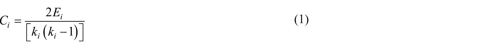
Table 3 summarized the built environment variables used in this study. Taking station A as an example, X1 represented the complexity of the road network, the formula for which was:

C_{i} = \frac{2 E_{i}}{[k_{i} (k_{i} - 1)]}

(1)

X 1 = \frac{1}{n} \sum_{i = 1}^{n} C_{i}

(2)

where $n$ is the total number of road network nodes in the PCA of A, $C_{i}$ represents the local clustering coefficient of node $i,$ $k_{i}$ indicates the number of nodes adjacent to node $i,$ and $E_{i}$ is the number of edges that exist between node i and its neighbors.

X2 was the mean shortest path length of road calculated by:

X 2 = \frac{1}{n (n - 1)} \sum_{i \neq j} d_{i j}

(3)

where $d_{ij}$ represents the shortest path from nodes i to j in the road network.

X6, the degree of a metro station, denoted the number of stations directly connected to A. Additionally, if the value of X7, the betweenness centrality of A, was larger, then the shortest paths between more stations in the metro system would pass through station A. The corresponding formula was as follows:

X 7 = \sum_{s \neq A \neq u} \frac{p (A)}{p}

(4)

where s and u indicate the other two metro stations. $p (A)$ is the number of shortest paths through A between $s$ and $u$ ; $p$ is the number of shortest paths between $s$ and $u$ .

Regression modeling of the built environment and public transit ridership variables

PLSR is a regression model mainly related to multiple linear regression, typical correlation analysis, and principal component analysis. It establishes a regression model between the $c$ -dimensional independent variables and $d$ -dimensional dependent variables by determining the principal components with higher interpretability. The basic model was described as follows:

X = T P^{T} + E

(5)

Y = U Q^{T} + F

(6)

where X is the independent variable and denotes the $N * c$ matrix, $N$ is the number of samples, $Y$ is the dependent variable and denotes the $N * d$ matrix, $T$ and $U$ are $N * r$ matrices that represent the score matrices of $X$ and $Y$ respectively, and $r$ is the number of principal components. $P$ ( $c * r$ matrix) and $Q$ ( $d * r$ matrix) are the loading matrices of $X$ and $Y,$ respectively. $E$ and $F$ indicate the residual matrices of $X$ and $Y,$ respectively.

The built environment and metro and taxi ridership variables were modeled by using an R package developed by Mevik and Wehrens (2007). Taking Y₁ in the t period of residential PCAs as an example, the formula was as follows:

y_{1}^{t} - \bar{y_{1}^{t}} = F_{t} (X)

(7)

where $y_{1}^{t}$ represents metro boarding in the $t$ period. $\bar{y_{1}^{t}}$ is the mean value of $y_{1}^{t}$ in all residential PCAs, and serves as a benchmark used to measure the relative boarding changes of different metro stations in the same category. $X$ indicates the built environment variables and $F_{t}$ is the relationship between the built environment variables and metro boarding in the $t$ period obtained by PLSR. Additionally, the number of principal components corresponding to the minimum average estimation sum of squares, acquired by cross-validation, was used as the parameter of PLSR.

The importance magnitude of built environment variables

VIP value was chosen to denote the importance magnitude of the built environment variables. It is an indicator of feature selection in PLSR and can be used to measure the relative importance and contribution of the independent variables to the dependent variables (Mehmood et al., 2012; Mukherjee et al., 2015). The formula for calculating the VIP of variable $j$ was as follows:

V I P_{j} = \sqrt{\frac{\sum_{f = 1}^{F} W_{j f}^{2} S S Y_{f} J}{S S Y_{T o t a l} F}}

(8)

where $J$ is the number of dependent variables $X$ , and $F$ is the number of components. $W_{j f}$ is the weight of variable $j$ and component $f .$ $S S Y_{f}$ is the sum of squares that is explained by the variance for component $f,$ and $S S Y_{T o t a l}$ is the total sum of squares that is explained by the dependent variables (Suo et al., 2018).

The threshold of VIP was usually set to 1, and an independent variable with a VIP value >1 was considered important, otherwise it was unimportant (Mehmood et al., 2012; Mukherjee et al., 2015; Suo et al., 2018). Therefore, when the VIP value of a built environment variable was >1, the variable was considered transferable with an important impact on the ridership. A larger VIP value denoted higher importance magnitude.

Public transit ridership estimation model and evaluation

TVs and all the built environment variables were used to estimate the metro and taxi ridership and their results were compared. Considering the estimation of Y₁ in the $t$ period in a residential PCA as an example, the formula for using TVs was:

\hat{y_{1}^{t}} = | \sum X_{1}^{t *} {W_{1}}^{t *} + \bar{y_{1}^{t}} |

(9)

where $\hat{y_{1}^{t}}$ is the estimated value of $y_{1}$ in the $t$ period, $X_{1}^{t *}$ represents the transferable built environment variables for metro boarding in the $t$ period, and ${W_{1}}^{t *}$ is the coefficient corresponding to each $X_{1}^{t *}$ in the $t$ period. When the estimation performed by considering all the built environment variables, $X$ and $W$ transformed accordingly.

In order to compare the performance of these two methods, 5-fold cross-validation was employed in the metro and taxi ridership estimation in each category of PCAs. The mean absolute error (MAE) and its percentage form MAE% was selected as the evaluation index. The formula of MAE% was shown as follows:

M A E % = \frac{M A E_{V I P} - M A E_{A l l}}{M A E_{A l l}} * 100 %

(10)

where $M A E_{V I P}$ and $M A E_{A l l}$ represent the MAE of the results estimated based on the TVs and all the built environment variables, respectively. The $M A E %$ indicates a relative improvement in accuracy, and a $M A E %$ <0 suggests that adopting TVs will improve the accuracy.

The calculation of MAE was given as:

M A E = \frac{1}{n} \sum_{i = 1}^{n} | q_{i} - \hat{q_{i}} |

(11)

where $n$ is the number of samples. $q_{i}$ and $\hat{q_{i}}$ are the true and estimation values of sample $i .$

Result and discussion

Analyzing the importance magnitude of the built environment variables on regression modeling of the metro and taxi ridership

This section discussed the importance magnitude of the built environment variables for the metro and taxi ridership from two aspects: time-varying law and sorting.

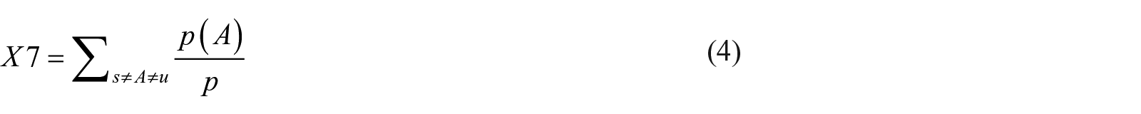
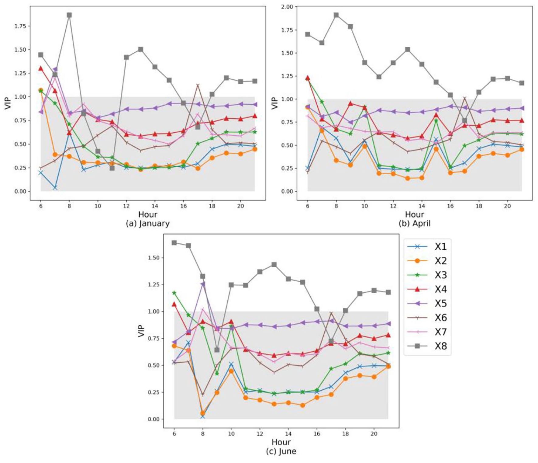
For time-varying, the importance magnitude of the built environment variables on the metro and taxi ridership changed over time. Figure 3 showed the hourly variation in the VIP values of X12 (financial insurance service POIs) and X14 (corporate enterprise POIs) for the metro and taxi ridership of work PCAs on Mondays in January, April and June, and Figure 4 demonstrates their situation on Saturdays for the same time frames. Additionally, the gray regions in these figures indicated that the VIP values were <1. For the metro ridership, as shown in Figure 3(a), the average VIP values of X12 and X14 for Y₁ (metro boarding) on Mondays were <1 during the peak morning hours (6:00–9:00) and reached their highest value (>1.1) for the day during 17:00–19:00, i.e., the peak evening hours. However, for Y₂ (metro alighting), their importance magnitude was highest in the peak morning hours, especially during 7:00–9:00 (VIP values of X12 >1.2 and X14 >1.1), and lowered (VIP values <1) after 17:00, which was opposite to that for Y₁. The period of relatively higher VIP values (>1.1) corresponded to that of a larger metro ridership in a day. The trend was similar to the variation of morning and evening peak metro ridership. Notably, such trend of X12 and X14 on Saturdays was the same but with lower VIP values. Nevertheless, compared to the metro ridership, there were mainly two difference of VIP values for the taxi ridership, as shown in Figure 3(b) and Figure 4(b). First, the VIP values of both X12 and X14 were >1 in almost all time periods, which indicated X12 and X14 had a lasting important influence on the taxi ridership. Second, the change trend of VIP values did not reflect characteristics of morning and evening peak. Although the trend was not very similar in different months like that for the metro ridership, there was a decreasing tendency of importance magnitude from morning to evening.

Figure 3.

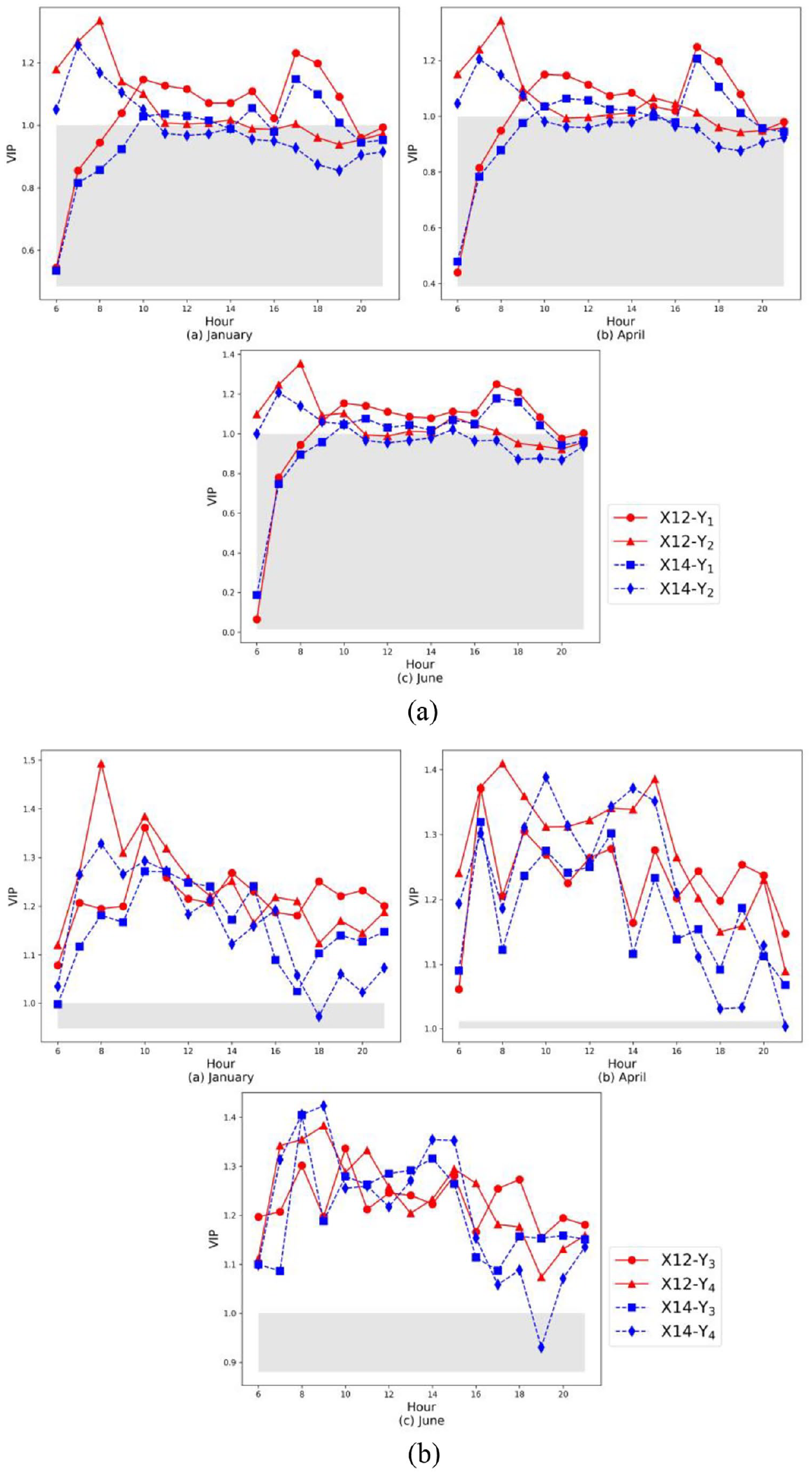
Changes in the VIP values of X12 and X14 for the metro and taxi ridership on Mondays in work PCAs.

Figure 4.

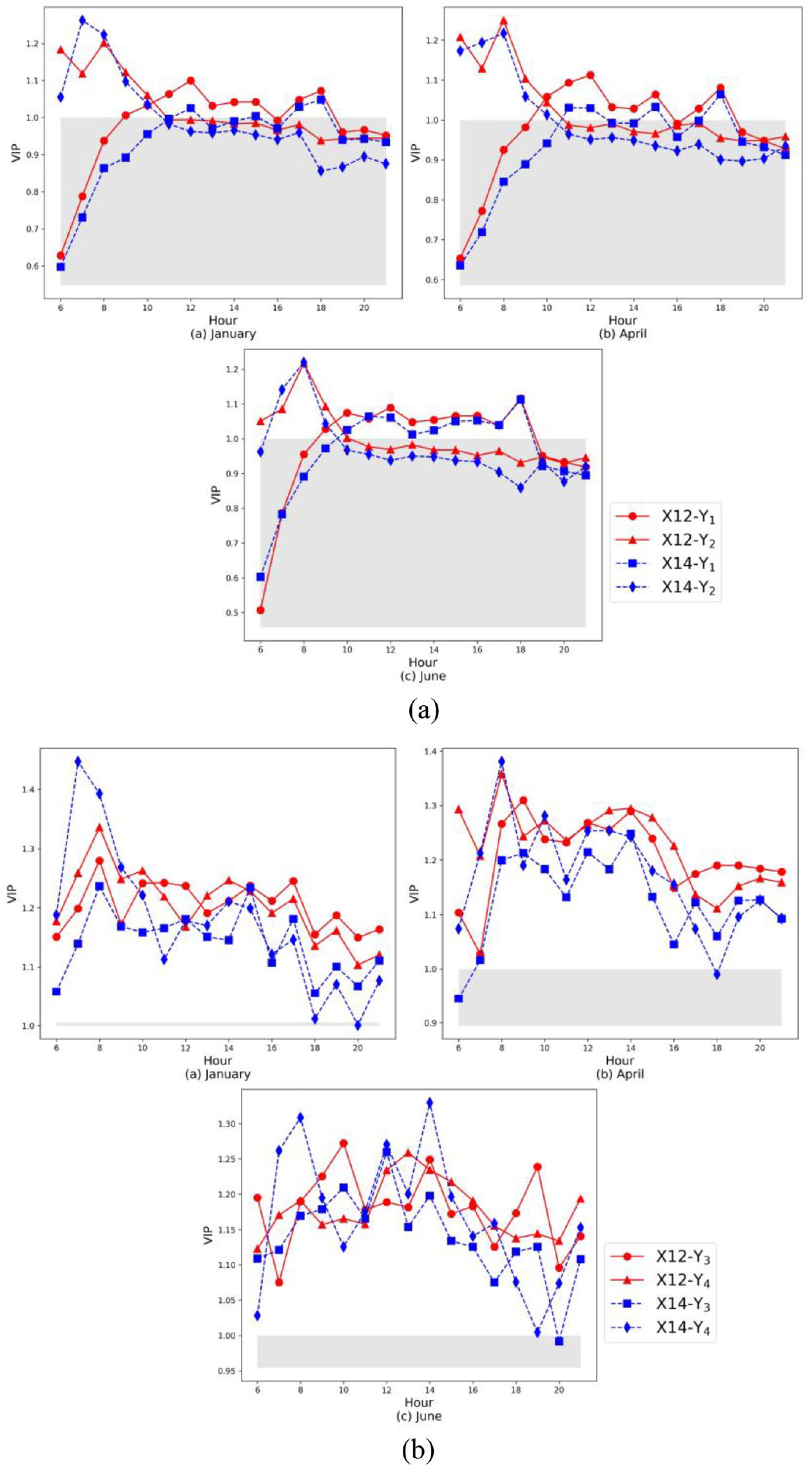
Changes in the VIP values of X12 and X14 for the metro and taxi ridership on Saturdays in work PCAs.

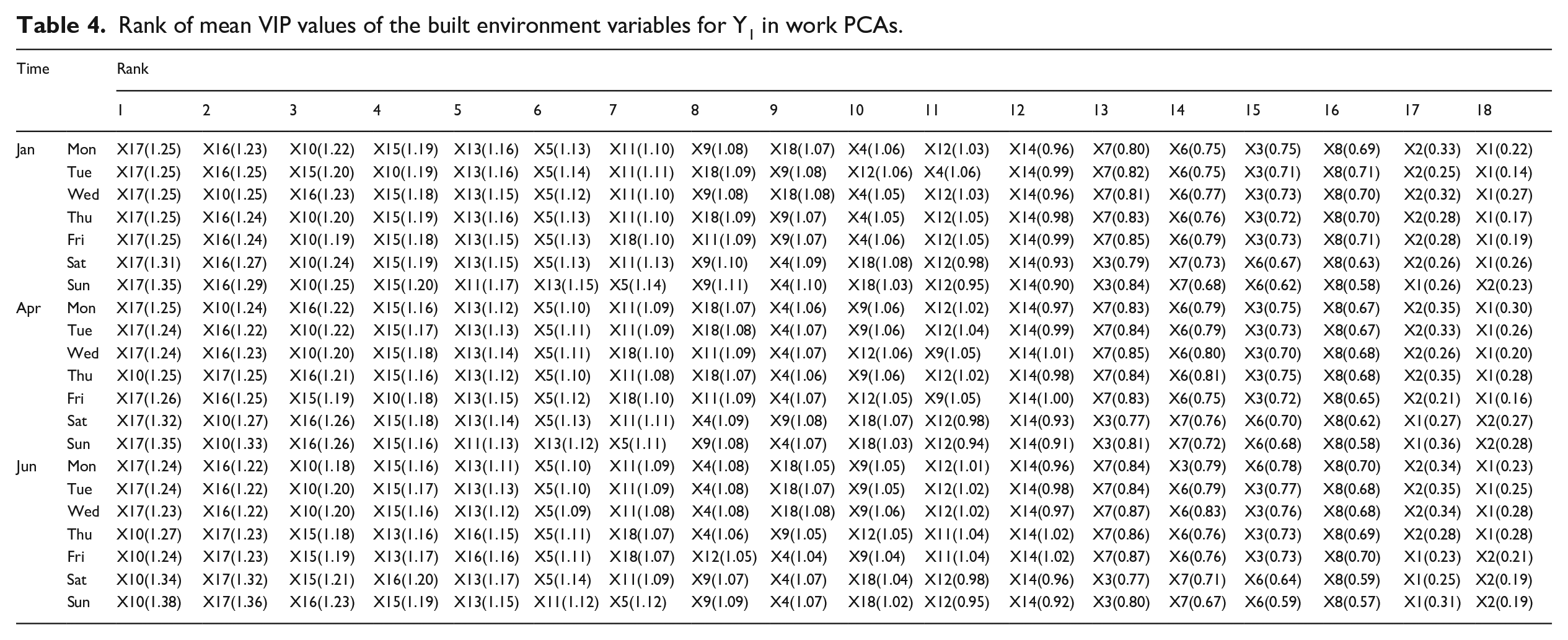
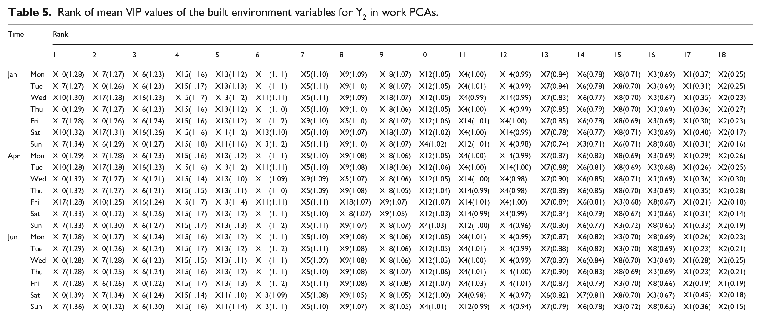
Two conclusions are also drawn in terms of sorting. Tables 4 and 5 showed the daily average importance magnitude of each built environment variable in work PCAs for Y₁ and Y₂, respectively. The magnitudes in other situations were shown in Appendix A. The values were mentioned in two decimal places; hence, there were cases where the ranks were different, but the values were the same.

On average, one or two (about 18%) variables in external connectivity, intermodal connection, population, station categories (non-land use categories, X1–X8) were important (mean VIP values >1) for the metro and taxi ridership. On the contrary, eight or nine (about 85%) land use variables showed important influence on the ridership. In general, the influence of land use variables on metro and taxi ridership was greater than that of non-land use ones.

Among all the built environment variables in this study, those with the highest importance magnitude for the metro and taxi ridership were independent of time (weeks, months), but were related to PCA categories and transportation modes. In residential PCAs, the most important variables in all variable categories for the metro and taxi ridership were X17 (accommodation services POIs) and X15 (serviced apartment POIs), respectively. Moreover, in non-land use category, only X8 (distance to the city center) and X5 (population size), with VIP values >1, separately showed an important influence on the metro and taxi ridership. In work PCAs, X10 (tourist attraction POIs) and X17 had the greatest impact on the metro ridership, while X18 (scientific and education service POIs) on the taxi ridership. Additionally, in non-land use category, X5 was the most important factor for both metro and taxi ridership.

Table 4.

Rank of mean VIP values of the built environment variables for Y₁ in work PCAs.

Time		Rank
Time		1	2	3	4	5	6	7	8	9	10	11	12	13	14	15	16	17	18
Jan	Mon	X17(1.25)	X16(1.23)	X10(1.22)	X15(1.19)	X13(1.16)	X5(1.13)	X11(1.10)	X9(1.08)	X18(1.07)	X4(1.06)	X12(1.03)	X14(0.96)	X7(0.80)	X6(0.75)	X3(0.75)	X8(0.69)	X2(0.33)	X1(0.22)
	Tue	X17(1.25)	X16(1.25)	X15(1.20)	X10(1.19)	X13(1.16)	X5(1.14)	X11(1.11)	X18(1.09)	X9(1.08)	X12(1.06)	X4(1.06)	X14(0.99)	X7(0.82)	X6(0.75)	X3(0.71)	X8(0.71)	X2(0.25)	X1(0.14)
	Wed	X17(1.25)	X10(1.25)	X16(1.23)	X15(1.18)	X13(1.15)	X5(1.12)	X11(1.10)	X9(1.08)	X18(1.08)	X4(1.05)	X12(1.03)	X14(0.96)	X7(0.81)	X6(0.77)	X3(0.73)	X8(0.70)	X2(0.32)	X1(0.27)
	Thu	X17(1.25)	X16(1.24)	X10(1.20)	X15(1.19)	X13(1.16)	X5(1.13)	X11(1.10)	X18(1.09)	X9(1.07)	X4(1.05)	X12(1.05)	X14(0.98)	X7(0.83)	X6(0.76)	X3(0.72)	X8(0.70)	X2(0.28)	X1(0.17)
	Fri	X17(1.25)	X16(1.24)	X10(1.19)	X15(1.18)	X13(1.15)	X5(1.13)	X18(1.10)	X11(1.09)	X9(1.07)	X4(1.06)	X12(1.05)	X14(0.99)	X7(0.85)	X6(0.79)	X3(0.73)	X8(0.71)	X2(0.28)	X1(0.19)
	Sat	X17(1.31)	X16(1.27)	X10(1.24)	X15(1.19)	X13(1.15)	X5(1.13)	X11(1.13)	X9(1.10)	X4(1.09)	X18(1.08)	X12(0.98)	X14(0.93)	X3(0.79)	X7(0.73)	X6(0.67)	X8(0.63)	X2(0.26)	X1(0.26)
	Sun	X17(1.35)	X16(1.29)	X10(1.25)	X15(1.20)	X11(1.17)	X13(1.15)	X5(1.14)	X9(1.11)	X4(1.10)	X18(1.03)	X12(0.95)	X14(0.90)	X3(0.84)	X7(0.68)	X6(0.62)	X8(0.58)	X1(0.26)	X2(0.23)
Apr	Mon	X17(1.25)	X10(1.24)	X16(1.22)	X15(1.16)	X13(1.12)	X5(1.10)	X11(1.09)	X18(1.07)	X4(1.06)	X9(1.06)	X12(1.02)	X14(0.97)	X7(0.83)	X6(0.79)	X3(0.75)	X8(0.67)	X2(0.35)	X1(0.30)
	Tue	X17(1.24)	X16(1.22)	X10(1.22)	X15(1.17)	X13(1.13)	X5(1.11)	X11(1.09)	X18(1.08)	X4(1.07)	X9(1.06)	X12(1.04)	X14(0.99)	X7(0.84)	X6(0.79)	X3(0.73)	X8(0.67)	X2(0.33)	X1(0.26)
	Wed	X17(1.24)	X16(1.23)	X10(1.20)	X15(1.18)	X13(1.14)	X5(1.11)	X18(1.10)	X11(1.09)	X4(1.07)	X12(1.06)	X9(1.05)	X14(1.01)	X7(0.85)	X6(0.80)	X3(0.70)	X8(0.68)	X2(0.26)	X1(0.20)
	Thu	X10(1.25)	X17(1.25)	X16(1.21)	X15(1.16)	X13(1.12)	X5(1.10)	X11(1.08)	X18(1.07)	X4(1.06)	X9(1.06)	X12(1.02)	X14(0.98)	X7(0.84)	X6(0.81)	X3(0.75)	X8(0.68)	X2(0.35)	X1(0.28)
	Fri	X17(1.26)	X16(1.25)	X15(1.19)	X10(1.18)	X13(1.15)	X5(1.12)	X18(1.10)	X11(1.09)	X4(1.07)	X12(1.05)	X9(1.05)	X14(1.00)	X7(0.83)	X6(0.75)	X3(0.72)	X8(0.65)	X2(0.21)	X1(0.16)
	Sat	X17(1.32)	X10(1.27)	X16(1.26)	X15(1.18)	X13(1.14)	X5(1.13)	X11(1.11)	X4(1.09)	X9(1.08)	X18(1.07)	X12(0.98)	X14(0.93)	X3(0.77)	X7(0.76)	X6(0.70)	X8(0.62)	X1(0.27)	X2(0.27)
	Sun	X17(1.35)	X10(1.33)	X16(1.26)	X15(1.16)	X11(1.13)	X13(1.12)	X5(1.11)	X9(1.08)	X4(1.07)	X18(1.03)	X12(0.94)	X14(0.91)	X3(0.81)	X7(0.72)	X6(0.68)	X8(0.58)	X1(0.36)	X2(0.28)
Jun	Mon	X17(1.24)	X16(1.22)	X10(1.18)	X15(1.16)	X13(1.11)	X5(1.10)	X11(1.09)	X4(1.08)	X18(1.05)	X9(1.05)	X12(1.01)	X14(0.96)	X7(0.84)	X3(0.79)	X6(0.78)	X8(0.70)	X2(0.34)	X1(0.23)
	Tue	X17(1.24)	X16(1.22)	X10(1.20)	X15(1.17)	X13(1.13)	X5(1.10)	X11(1.09)	X4(1.08)	X18(1.07)	X9(1.05)	X12(1.02)	X14(0.98)	X7(0.84)	X6(0.79)	X3(0.77)	X8(0.68)	X2(0.35)	X1(0.25)
	Wed	X17(1.23)	X16(1.22)	X10(1.20)	X15(1.16)	X13(1.12)	X5(1.09)	X11(1.08)	X4(1.08)	X18(1.08)	X9(1.06)	X12(1.02)	X14(0.97)	X7(0.87)	X6(0.83)	X3(0.76)	X8(0.68)	X2(0.34)	X1(0.28)
	Thu	X10(1.27)	X17(1.23)	X15(1.18)	X13(1.16)	X16(1.15)	X5(1.11)	X18(1.07)	X4(1.06)	X9(1.05)	X12(1.05)	X11(1.04)	X14(1.02)	X7(0.86)	X6(0.76)	X3(0.73)	X8(0.69)	X2(0.28)	X1(0.28)
	Fri	X10(1.24)	X17(1.23)	X15(1.19)	X13(1.17)	X16(1.16)	X5(1.11)	X18(1.07)	X12(1.05)	X4(1.04)	X9(1.04)	X11(1.04)	X14(1.02)	X7(0.87)	X6(0.76)	X3(0.73)	X8(0.70)	X1(0.23)	X2(0.21)
	Sat	X10(1.34)	X17(1.32)	X15(1.21)	X16(1.20)	X13(1.17)	X5(1.14)	X11(1.09)	X9(1.07)	X4(1.07)	X18(1.04)	X12(0.98)	X14(0.96)	X3(0.77)	X7(0.71)	X6(0.64)	X8(0.59)	X1(0.25)	X2(0.19)
	Sun	X10(1.38)	X17(1.36)	X16(1.23)	X15(1.19)	X13(1.15)	X11(1.12)	X5(1.12)	X9(1.09)	X4(1.07)	X18(1.02)	X12(0.95)	X14(0.92)	X3(0.80)	X7(0.67)	X6(0.59)	X8(0.57)	X1(0.31)	X2(0.19)

Table 5.

Rank of mean VIP values of the built environment variables for Y₂ in work PCAs.

Time		Rank
Time		1	2	3	4	5	6	7	8	9	10	11	12	13	14	15	16	17	18
Jan	Mon	X10(1.28)	X17(1.27)	X16(1.23)	X15(1.16)	X13(1.12)	X11(1.11)	X5(1.10)	X9(1.09)	X18(1.07)	X12(1.05)	X4(1.00)	X14(0.99)	X7(0.84)	X6(0.78)	X8(0.71)	X3(0.69)	X1(0.37)	X2(0.25)
	Tue	X17(1.27)	X10(1.26)	X16(1.23)	X15(1.17)	X13(1.13)	X11(1.11)	X5(1.11)	X9(1.10)	X18(1.07)	X12(1.05)	X4(1.01)	X14(0.99)	X7(0.84)	X6(0.78)	X8(0.70)	X3(0.69)	X1(0.31)	X2(0.25)
	Wed	X10(1.30)	X17(1.28)	X16(1.23)	X15(1.17)	X13(1.12)	X11(1.11)	X5(1.11)	X9(1.09)	X18(1.07)	X12(1.05)	X4(0.99)	X14(0.99)	X7(0.83)	X6(0.77)	X8(0.70)	X3(0.67)	X1(0.35)	X2(0.23)
	Thu	X10(1.29)	X17(1.27)	X16(1.23)	X15(1.16)	X13(1.12)	X11(1.10)	X5(1.10)	X9(1.10)	X18(1.06)	X12(1.05)	X4(1.00)	X14(0.99)	X7(0.85)	X6(0.79)	X8(0.70)	X3(0.69)	X1(0.36)	X2(0.27)
	Fri	X17(1.28)	X10(1.26)	X16(1.24)	X15(1.16)	X13(1.12)	X11(1.12)	X9(1.10)	X5(1.10)	X18(1.07)	X12(1.06)	X14(1.01)	X4(1.00)	X7(0.85)	X6(0.78)	X8(0.69)	X3(0.69)	X1(0.30)	X2(0.23)
	Sat	X10(1.32)	X17(1.31)	X16(1.26)	X15(1.16)	X11(1.12)	X13(1.10)	X5(1.10)	X9(1.07)	X18(1.07)	X12(1.02)	X4(1.00)	X14(0.99)	X7(0.78)	X6(0.77)	X8(0.71)	X3(0.69)	X1(0.40)	X2(0.17)
	Sun	X17(1.34)	X16(1.29)	X10(1.27)	X15(1.18)	X11(1.16)	X13(1.12)	X5(1.11)	X9(1.10)	X18(1.07)	X4(1.02)	X12(1.01)	X14(0.98)	X7(0.74)	X3(0.71)	X6(0.71)	X8(0.68)	X1(0.31)	X2(0.16)
Apr	Mon	X10(1.29)	X17(1.28)	X16(1.23)	X15(1.16)	X13(1.12)	X11(1.11)	X5(1.10)	X9(1.08)	X18(1.06)	X12(1.05)	X4(1.00)	X14(0.99)	X7(0.87)	X6(0.82)	X8(0.69)	X3(0.69)	X1(0.29)	X2(0.26)
	Tue	X10(1.28)	X17(1.28)	X16(1.23)	X15(1.16)	X13(1.12)	X11(1.11)	X5(1.10)	X9(1.08)	X18(1.06)	X12(1.06)	X4(1.00)	X14(1.00)	X7(0.88)	X6(0.81)	X8(0.69)	X3(0.68)	X1(0.26)	X2(0.25)
	Wed	X10(1.32)	X17(1.27)	X16(1.21)	X15(1.14)	X13(1.10)	X11(1.09)	X9(1.09)	X5(1.07)	X18(1.06)	X12(1.05)	X14(1.00)	X4(0.98)	X7(0.90)	X6(0.85)	X8(0.71)	X3(0.69)	X1(0.36)	X2(0.30)
	Thu	X10(1.32)	X17(1.27)	X16(1.21)	X15(1.15)	X13(1.11)	X11(1.10)	X5(1.09)	X9(1.08)	X18(1.05)	X12(1.04)	X14(0.99)	X4(0.98)	X7(0.89)	X6(0.85)	X8(0.70)	X3(0.69)	X1(0.35)	X2(0.28)
	Fri	X17(1.28)	X10(1.25)	X16(1.24)	X15(1.17)	X13(1.14)	X11(1.11)	X5(1.11)	X18(1.07)	X9(1.07)	X12(1.07)	X14(1.01)	X4(1.00)	X7(0.89)	X6(0.81)	X3(0.68)	X8(0.67)	X1(0.21)	X2(0.18)
	Sat	X17(1.33)	X10(1.32)	X16(1.26)	X15(1.17)	X13(1.12)	X11(1.11)	X5(1.10)	X18(1.07)	X9(1.05)	X12(1.03)	X14(0.99)	X4(0.99)	X7(0.84)	X6(0.79)	X8(0.67)	X3(0.66)	X1(0.31)	X2(0.14)
	Sun	X17(1.33)	X10(1.30)	X16(1.27)	X15(1.17)	X13(1.13)	X11(1.12)	X5(1.11)	X9(1.07)	X18(1.07)	X4(1.03)	X12(1.00)	X14(0.96)	X7(0.80)	X6(0.77)	X3(0.72)	X8(0.65)	X1(0.33)	X2(0.19)
Jun	Mon	X17(1.28)	X10(1.27)	X16(1.24)	X15(1.16)	X13(1.12)	X11(1.11)	X5(1.10)	X9(1.08)	X18(1.06)	X12(1.05)	X4(1.01)	X14(0.99)	X7(0.87)	X6(0.82)	X3(0.70)	X8(0.69)	X1(0.26)	X2(0.23)
	Tue	X17(1.29)	X10(1.26)	X16(1.24)	X15(1.17)	X13(1.12)	X11(1.12)	X5(1.11)	X9(1.08)	X18(1.06)	X12(1.05)	X4(1.01)	X14(0.99)	X7(0.88)	X6(0.82)	X3(0.70)	X8(0.69)	X1(0.23)	X2(0.21)
	Wed	X10(1.28)	X17(1.28)	X16(1.23)	X15(1.15)	X13(1.11)	X11(1.11)	X5(1.09)	X9(1.08)	X18(1.06)	X12(1.05)	X4(1.00)	X14(0.99)	X7(0.89)	X6(0.84)	X8(0.70)	X3(0.69)	X1(0.28)	X2(0.25)
	Thu	X17(1.28)	X10(1.25)	X16(1.24)	X15(1.16)	X13(1.12)	X11(1.11)	X5(1.10)	X9(1.08)	X18(1.07)	X12(1.06)	X4(1.01)	X14(1.00)	X7(0.90)	X6(0.83)	X8(0.69)	X3(0.69)	X1(0.23)	X2(0.21)
	Fri	X17(1.28)	X16(1.26)	X10(1.22)	X15(1.17)	X13(1.13)	X11(1.12)	X5(1.11)	X9(1.08)	X18(1.08)	X12(1.07)	X4(1.03)	X14(1.01)	X7(0.87)	X6(0.79)	X3(0.70)	X8(0.66)	X2(0.19)	X1(0.19)
	Sat	X10(1.39)	X17(1.34)	X16(1.24)	X15(1.14)	X11(1.10)	X13(1.09)	X5(1.08)	X9(1.05)	X18(1.05)	X12(1.00)	X4(0.98)	X14(0.97)	X6(0.82)	X7(0.81)	X8(0.70)	X3(0.67)	X1(0.45)	X2(0.18)
	Sun	X17(1.36)	X10(1.32)	X16(1.30)	X15(1.16)	X11(1.14)	X13(1.11)	X5(1.10)	X9(1.07)	X18(1.05)	X4(1.01)	X12(0.99)	X14(0.94)	X7(0.79)	X6(0.78)	X3(0.72)	X8(0.65)	X1(0.36)	X2(0.15)

Analysis of TVs for the metro and taxi ridership

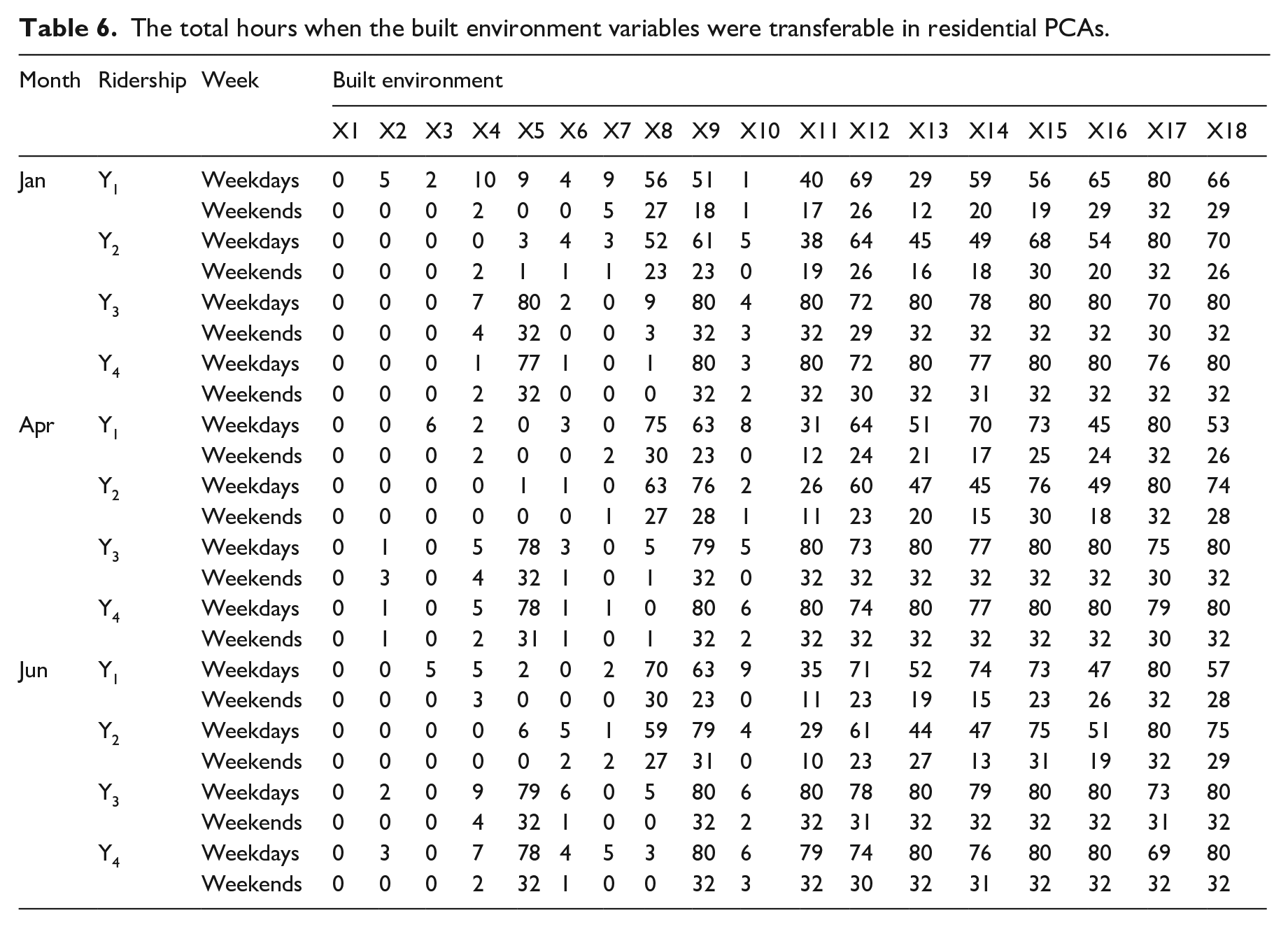
This section has discussed the transferability magnitude of the built environment variables. The built environment variables (VIP values >1) were considered to have important influence on the ridership, so they were thought transferable and applicable to be used to estimate the ridership in other PCAs of the same category. Variables maintaining important influence (VIP values >1) for longer periods indicated they had higher transferability magnitude.

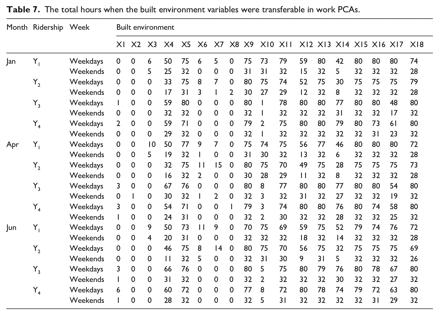
Tables 6 and 7 show the number of hours when each built environment variable of residential and work PCAs was transferable on weekdays (Monday to Friday; 80 hours) and weekends (Saturday and Sunday; 32 hours), respectively. In work PCAs, from the aspects of time and traffic modes, about 85% of the land use variables were found to be transferable at least 70% of the time (including weekdays and weekends), and the non-land use variables accounted for almost 19%, while they were about 72% of the land use variables and 12% of the non-land use ones in residential PCAs. This indicated that most land use variables were highly transferable, and served as key factors affecting the metro and taxi ridership. However, most non-land use variables showed low transferability magnitude. The last section illustrated that although the mean VIP values of most non-land use variables were <1, indicating their overall slight influence, they showed important impact on the ridership in some periods. For example, during 6:00–7:00 on Mondays in residential PCAs, the VIP values of X3 (number of bus stations) and X4 (number of bus lines) for Y₁ were >1 (Figure 5).

Table 6.

The total hours when the built environment variables were transferable in residential PCAs.

Month	Ridership	Week	Built environment
Month	Ridership	Week	X1	X2	X3	X4	X5	X6	X7	X8	X9	X10	X11	X12	X13	X14	X15	X16	X17	X18
Jan	Y₁	Weekdays	0	5	2	10	9	4	9	56	51	1	40	69	29	59	56	65	80	66
	Y₁	Weekends	0	0	0	2	0	0	5	27	18	1	17	26	12	20	19	29	32	29
	Y₂	Weekdays	0	0	0	0	3	4	3	52	61	5	38	64	45	49	68	54	80	70
	Y₂	Weekends	0	0	0	2	1	1	1	23	23	0	19	26	16	18	30	20	32	26
	Y₃	Weekdays	0	0	0	7	80	2	0	9	80	4	80	72	80	78	80	80	70	80
	Y₃	Weekends	0	0	0	4	32	0	0	3	32	3	32	29	32	32	32	32	30	32
	Y₄	Weekdays	0	0	0	1	77	1	0	1	80	3	80	72	80	77	80	80	76	80
	Y₄	Weekends	0	0	0	2	32	0	0	0	32	2	32	30	32	31	32	32	32	32
Apr	Y₁	Weekdays	0	0	6	2	0	3	0	75	63	8	31	64	51	70	73	45	80	53
	Y₁	Weekends	0	0	0	2	0	0	2	30	23	0	12	24	21	17	25	24	32	26
	Y₂	Weekdays	0	0	0	0	1	1	0	63	76	2	26	60	47	45	76	49	80	74
	Y₂	Weekends	0	0	0	0	0	0	1	27	28	1	11	23	20	15	30	18	32	28
	Y₃	Weekdays	0	1	0	5	78	3	0	5	79	5	80	73	80	77	80	80	75	80
	Y₃	Weekends	0	3	0	4	32	1	0	1	32	0	32	32	32	32	32	32	30	32
	Y₄	Weekdays	0	1	0	5	78	1	1	0	80	6	80	74	80	77	80	80	79	80
	Y₄	Weekends	0	1	0	2	31	1	0	1	32	2	32	32	32	32	32	32	30	32
Jun	Y₁	Weekdays	0	0	5	5	2	0	2	70	63	9	35	71	52	74	73	47	80	57
	Y₁	Weekends	0	0	0	3	0	0	0	30	23	0	11	23	19	15	23	26	32	28
	Y₂	Weekdays	0	0	0	0	6	5	1	59	79	4	29	61	44	47	75	51	80	75
	Y₂	Weekends	0	0	0	0	0	2	2	27	31	0	10	23	27	13	31	19	32	29
	Y₃	Weekdays	0	2	0	9	79	6	0	5	80	6	80	78	80	79	80	80	73	80
	Y₃	Weekends	0	0	0	4	32	1	0	0	32	2	32	31	32	32	32	32	31	32
	Y₄	Weekdays	0	3	0	7	78	4	5	3	80	6	79	74	80	76	80	80	69	80
	Y₄	Weekends	0	0	0	2	32	1	0	0	32	3	32	30	32	31	32	32	32	32

Table 7.

The total hours when the built environment variables were transferable in work PCAs.

Month	Ridership	Week	Built environment
Month	Ridership	Week	X1	X2	X3	X4	X5	X6	X7	X8	X9	X10	X11	X12	X13	X14	X15	X16	X17	X18
Jan	Y₁	Weekdays	0	0	6	50	75	6	5	0	75	73	79	59	80	42	80	80	80	74
	Y₁	Weekends	0	0	5	25	32	0	0	0	31	31	32	15	32	5	32	32	32	28
	Y₂	Weekdays	0	0	0	33	75	8	7	0	80	75	74	52	75	30	75	75	75	79
	Y₂	Weekends	0	0	0	17	31	3	1	2	30	27	29	12	32	8	32	32	32	28
	Y₃	Weekdays	1	0	0	59	80	0	0	0	80	1	78	80	80	77	80	80	48	80
	Y₃	Weekends	0	0	0	32	32	0	0	0	32	1	32	32	32	31	32	32	17	32
	Y₄	Weekdays	2	0	0	59	71	0	0	0	79	2	75	80	80	79	80	73	61	80
	Y₄	Weekends	0	0	0	29	32	0	0	0	32	1	32	32	32	32	32	31	23	32
Apr	Y₁	Weekdays	0	0	10	50	77	9	7	0	75	74	75	56	77	46	80	80	80	72
	Y₁	Weekends	0	0	5	19	32	1	0	0	31	30	32	13	32	6	32	32	32	28
	Y₂	Weekdays	0	0	0	32	75	11	15	0	80	75	70	49	75	28	75	75	75	73
	Y₂	Weekends	0	0	0	16	32	2	0	0	30	28	29	11	32	8	32	32	32	28
	Y₃	Weekdays	3	0	0	67	76	0	0	0	80	8	77	80	80	77	80	80	54	80
	Y₃	Weekends	0	1	0	30	32	1	2	0	32	3	32	31	32	27	32	32	19	32
	Y₄	Weekdays	3	0	0	54	71	0	0	1	79	3	74	80	80	76	80	74	58	80
	Y₄	Weekends	1	0	0	24	31	0	0	0	32	2	30	32	32	28	32	32	25	32
Jun	Y₁	Weekdays	0	0	9	50	73	11	9	0	70	75	69	59	75	52	79	74	76	72
	Y₁	Weekends	0	0	4	20	31	0	0	0	32	32	32	18	32	14	32	32	32	28
	Y₂	Weekdays	0	0	0	46	75	8	14	0	80	75	70	56	75	32	75	75	75	69
	Y₂	Weekends	0	0	0	11	32	5	0	0	32	31	30	9	31	5	32	32	32	26
	Y₃	Weekdays	3	0	0	66	76	0	0	0	80	5	75	80	79	76	80	78	67	80
	Y₃	Weekends	1	0	0	31	32	0	0	0	32	2	32	32	32	30	32	32	27	32
	Y₄	Weekdays	6	0	0	60	72	0	0	0	77	8	72	80	78	74	79	72	63	80
	Y₄	Weekends	1	0	0	28	32	0	0	0	32	5	31	32	32	32	32	31	29	32

Figure 5.

Change in the importance magnitude of non-land use variables for Y₁ on Mondays in residential PCAs.

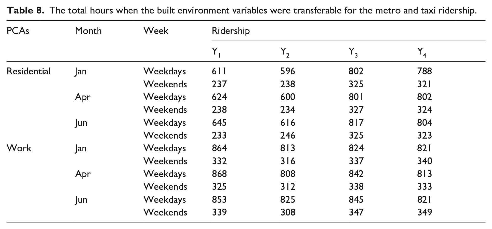
Transferability magnitude of the built environment variables was jointly affected by PCA categories and traffic modes. Table 8 showed the comparison of total hours when the built environment variables were transferable for the metro and taxi ridership on weekdays and weekends in three months. In residential PCAs, transferable duration for the metro ridership was remarkably less than that for the taxi ridership. The average time difference was about 187 hours on weekdays and 87 hours on weekends. Both accounted for nearly 28% of the average duration of the metro ridership in the corresponding time period (weekdays or weekends). This suggested that the VIP values for the taxi ridership remaining >1 tended to be more lasting and stable. Additionally, the VIP values for the metro ridership were susceptible to the morning and evening peak periods, such as X12 and X14 (the last section). The transferable durations for the metro and taxi ridership were similar in work PCAs, with difference accounting for about 3% of the mean duration for the metro ridership on weekdays and 6% on weekends. Furthermore, the total hours when the built environment variables were transferable for the metro and taxi ridership in work PCAs were more than those in residential PCAs, especially for the metro ridership. The time difference reflected that the built environment variables in work PCAs maintained a key influence on the metro and taxi ridership for a longer time period.

Table 8.

The total hours when the built environment variables were transferable for the metro and taxi ridership.

PCAs	Month	Week	Ridership
PCAs	Month	Week	Y₁	Y₂	Y₃	Y₄
Residential	Jan	Weekdays	611	596	802	788
	Jan	Weekends	237	238	325	321
	Apr	Weekdays	624	600	801	802
	Apr	Weekends	238	234	327	324
	Jun	Weekdays	645	616	817	804
	Jun	Weekends	233	246	325	323
Work	Jan	Weekdays	864	813	824	821
	Jan	Weekends	332	316	337	340
	Apr	Weekdays	868	808	842	813
	Apr	Weekends	325	312	338	333
	Jun	Weekdays	853	825	845	821
	Jun	Weekends	339	308	347	349

Comparative analysis of the estimation results of the metro and taxi ridership in PCAs

The metro and taxi ridership were estimated with TVs and all the built environment variables respectively based on 5-fold cross-validation, and their results were compared. This section illustrated the estimation of the average daily ridership. The specific estimation models of one fold for estimating the average daily metro and taxi ridership on Monday and Saturday in January in residential PCAs using Equation (9) are shown in Table 9 as an example.

Table 9.

Estimation models of the average daily metro and taxi ridership on Monday and Saturday in January in residential PCAs.

Ridership	Day	Models
Y₁	Mon.	$\hat{y_{1}} = \| \begin{array}{l} 0.07 * X 11 + 1.27 * X 12 + 0.52 * X 14 + \\ 1.19 * X 16 + 1.10 * X 17 + 0.74 * X 18 + \bar{y_{1}} \end{array} \|$
Y₁	Sat	$\hat{y_{1}} = \| \begin{array}{l} 0.06 * X 8 - 1.60 * X 9 + 2.71 * X 12 - 0.81 * X 13 - 0.54 * X 15 + \\ 4.43 * X 17 + 1.58 * X 18 + \bar{y_{1}} \end{array} \|$
Y₂	Mon.	$\hat{y_{2}} = \| \begin{array}{l} 0.08 * X 11 + 1.29 * X 12 + 0.54 * X 14 + 0.59 * X 15 + \\ 1.20 * X 16 + 1.10 * X 17 + 0.75 * X 18 + \bar{y_{2}} \end{array} \|$
Y₂	Sat	$\hat{y_{2}} = \| \begin{array}{l} 0.08 * X 11 + 1.13 * X 12 + 0.48 * X 14 + 0.53 * X 15 + \\ 1.11 * X 16 - 1.06 * X 17 + 0.69 * X 18 + \bar{y_{2}} \end{array} \|$
Y₃	Mon.	$\hat{y_{3}} = \| \begin{array}{l} (1.18 E - 04) * X 5 + 0.05 * X 9 + (3.56 E - 03) * X 11 + 0.05 * X 12 + 0.03 * X 13 + \\ 0.02 * X 14 + 0.04 * X 15 + 0.05 * X 16 + 0.03 * X 17 + 0.03 * X 18 + \bar{y_{3}} \end{array} \|$
Y₃	Sat	$\hat{y_{3}} = \| \begin{array}{l} (1.17 E - 04) * X 5 + 0.05 * X 9 + (3.46 E - 03) * X 11 + 0.05 * X 12 + 0.03 * X 13 + \\ 0.02 * X 14 + 0.04 * X 15 + 0.06 * X 16 + 0.03 * X 17 + 0.03 * X 18 + \bar{y_{3}} \end{array} \|$
Y₄	Mon.	$\hat{y_{4}} = \| \begin{array}{l} (1.14 E - 04) * X 5 + 0.05 * X 9 + (3.54 E - 03) * X 11 + 0.05 * X 12 + 0.03 * \\ X 13 + 0.02 * X 14 + 0.04 * X 15 + 0.05 * X 16 + 0.03 * X 17 + 0.03 * X 18 + \bar{y_{4}} \end{array} \|$
Y₄	Sat	$\hat{y_{4}} = \| \begin{array}{l} (1.12 E - 04) * X 5 + 0.05 * X 9 + (3.53 E - 03) * X 11 + 0.05 * X 12 + 0.03 * X 13 + \\ 0.02 * X 14 + 0.04 * X 15 + 0.06 * X 16 + 0.03 * X 17 + 0.03 * X 18 + \bar{y_{4}} \end{array} \|$

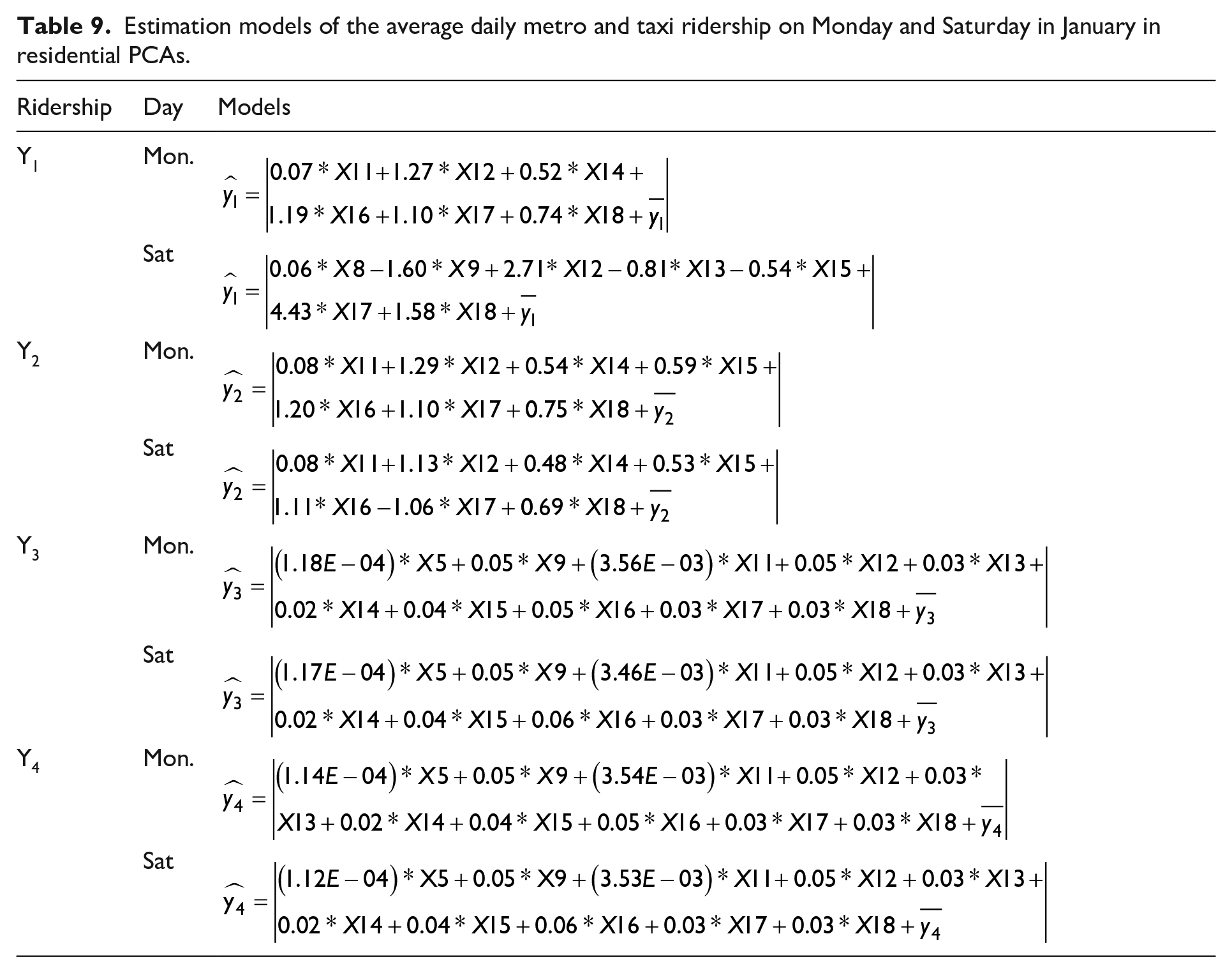
Table 10 showed the average performance of the metro and taxi ridership estimations on weekdays and weekends in work and residential PCAs, where the value column represented the actual values, and the MAE_A and MAE_T columns showed the MAE of the results estimated by all the built environment variables and TVs, respectively. Besides, the MAE% column, calculated by Equation (10), revealed the relative improvement in the accuracy of the ridership estimation.

Table 10.

Average performances of the metro and taxi ridership estimation in residential and work PCAs.

Month	PCAs	Week	Ridership
			Y₁				Y₂				Y₃				Y₄
			Value	MAE_A	MAE_T	MAE%	Value	MAE_A	MAE_T	MAE%	Value	MAE_A	MAE_T	MAE%	Value	MAE_A	MAE_T	MAE%
Jan	Work	Weekdays	597.33	855.24	705.93	–17.46	627.99	930.53	782.80	–15.88	13.02	31.36	26.18	–16.52	12.71	28.88	23.98	–16.96
	Work	Weekends	551.24	908.42	742.84	–18.23	561.49	1001.38	807.12	–19.40	13.06	30.88	26.11	–15.46	12.23	28.64	24.51	–14.43
	Residential	Weekdays	434.88	915.64	663.16	–27.57	412.52	839.19	625.24	–25.49	26.98	29.29	23.14	–20.99	25.15	27.96	22.04	–21.17
	Residential	Weekends	359.75	773.64	645.56	–16.56	334.61	679.01	561.74	–17.27	26.49	27.51	21.89	–20.43	24.81	26.08	20.67	–20.73
Apr	Work	Weekdays	638.60	940.88	785.72	–16.49	649.68	1022.84	849.71	–16.93	8.32	22.04	17.69	–19.77	8.45	20.96	17.45	–16.74
	Work	Weekends	576.10	1027.86	825.33	–19.70	571.92	1117.67	863.45	–22.75	8.73	21.54	17.78	–17.47	8.74	20.82	17.37	–16.55
	Residential	Weekdays	521.51	1071.38	734.76	–31.42	494.97	1052.43	729.46	–30.69	19.67	21.68	16.36	–24.54	18.10	19.38	15.32	–20.92
	Residential	Weekends	421.49	916.73	748.43	–18.36	396.07	897.15	791.26	–11.80	20.02	19.66	15.72	–20.08	17.91	18.14	14.05	–22.55
Jun	Work	Weekdays	597.60	846.54	718.85	–15.08	657.53	925.37	773.80	–16.38	6.73	15.77	13.17	–16.48	6.76	15.20	12.60	–17.08
	Work	Weekends	572.95	940.35	766.95	–18.44	608.39	1260.08	874.15	–30.63	6.21	15.03	13.00	–13.47	6.15	14.33	12.63	–11.85
	Residential	Weekdays	520.97	1010.51	679.43	–32.76	498.04	982.48	709.69	–27.77	14.47	15.44	12.09	–21.68	13.68	14.61	11.57	–20.82
	Residential	Weekends	444.81	897.74	727.91	–18.92	413.64	907.22	788.06	–13.13	14.15	14.47	11.44	–20.91	13.74	13.68	10.84	–20.78

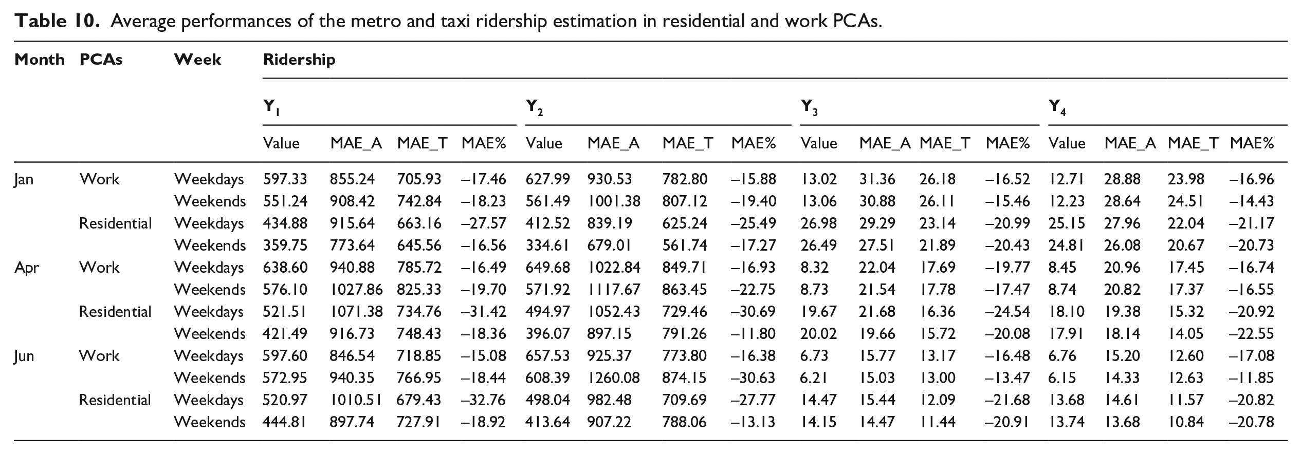
The improvement in estimation accuracy was affected by transportation types and PCA categories. From the aspect of transportation types, in residential and work PCAs, the average accuracy improvement for the metro ridership estimation based on TVs on weekdays and weekends was greater than that for the taxi ridership estimation. As shown in Table 10, the average improvement for the metro ridership (Y₁ and Y₂) prediction in January, April, and June was 19.73%, 21.02%, and 21.64% respectively, while that for the taxi ridership (Y₃ and Y₄) prediction was 18.33%, 19.83%, and 17.88%. Additionally, from the aspect of PCA categories, more accurate results were achieved for both ridership in residential PCAs. In residential PCAs, all the average improvement for the metro and taxi ridership were 22.65% and 21.30%, which was greater than those in work ones (18.95% and 16.06%). Besides, in each category of PCAs, the MAE% of the metro or taxi ridership estimation were similar in each month, which meant the accuracy improvement was not significantly related to the weather. Therefore, the improvement of estimating the metro and taxi ridership in different categories of PCAs were different, with the more obvious in residential PCAs. Besides, it was inferred that the ridership estimation error based on TVs was smaller than that based on all the built environment variables, with an average decrease of about 20% and 18% for the metro and taxi one respectively.

Conclusion

This study adopted PLSR to explore the importance magnitude of each built environment variable for the metro and taxi ridership in residential and work PCAs and the change in transferability magnitude with time, and then evaluated the estimation performance with TVs. The main conclusions drawn from this study were as follows: first, the importance magnitude of the built environment variables varied over time. The magnitude variation tendencies were mainly affected by PCA categories and traffic modes, and were generally similar in different seasons. Most of land use variables (about 85%) had a key impact on the metro and taxi ridership, while only around 18% of variables non-land use variables had important influence on the ridership. In residential PCAs, the vital built environment variables for the metro and taxi ridership were X17 (accommodation service POIs) and X15 (serviced apartment POIs), respectively. Besides, they were X10 (tourist attraction POIs) and X17 for the metro ridership, and X18 (scientific and education service POIs) for the taxi ridership in work PCAs. Notably, in residential PCAs, X8 (distance to the city center) and X5 (population size) had important influence on the metro and taxi ridership respectively, although the overall VIP values of non-land use variables were small. Additionally, in non-land use category of work PCAs, X5 was the most important factor for the metro and taxi ridership.

Second, in more than half of the time, nearly 80% land use variables were highly transferable, while around 85% non-land use variables showed low transferability magnitude. Highly important variables were generally highly transferable. In residential PCAs, the total number of hours when the built environment variables were transferable for the taxi ridership was greater than that for the metro ridership, while they were similar in work PCAs. Additionally, in work PCAs, the transferable time for the metro and taxi ridership was more than that in residential PCAs, especially for metro ridership.

Third, the estimation accuracy based on TVs was 20% for the metro ridership and 18% for the taxi one respectively higher than that based on all the built environment variables, even though the ridership varied in different categories of PCAs.

Based on the analysis of this study, some policy implications could be summarized as follows:

The VIP variation tendencies of X12 (financial insurance service POIs) and X14 (corporate enterprise POIs) for metro ridership also had obvious characteristics of peak hours in the morning and evening on weekends, instead of only on weekdays. This implied that in such PCAs, the metro management department should also pay attention to the ridership change on weekends during the peak hours and imply the ridership control measures in time.

Land use variables were the main factors that influencing changes of public transit ridership, which suggested there is no need to pay too much attention to non-land use variables, such as bus stops, in PCAs.

Predicting public transit ridership based on the TVs achieved more accurate results than those based on all variables. In order to reduce error, planners could use this method or idea proposed in this study to estimate when planning a new metro station in cities.

This study focused on the metro and taxi ridership in Wuhan, China. However, due to the data limitation, low-carbon traffic modes, such as shared bikes and electric vehicles, are not considered in this study. With the booming of sharing economy, such traffic modes will bring significant influence on the traffic and economic development. Therefore, it is important to include them in future analysis, which will help to understand the interaction between built environment and public transit ridership more comprehensively. Additionally, the importance and transferability magnitude of the built environment for public transit ridership in other cities should also be explored in order to verify the validity if the data is available.

Footnotes

Appendix A

Table A6.

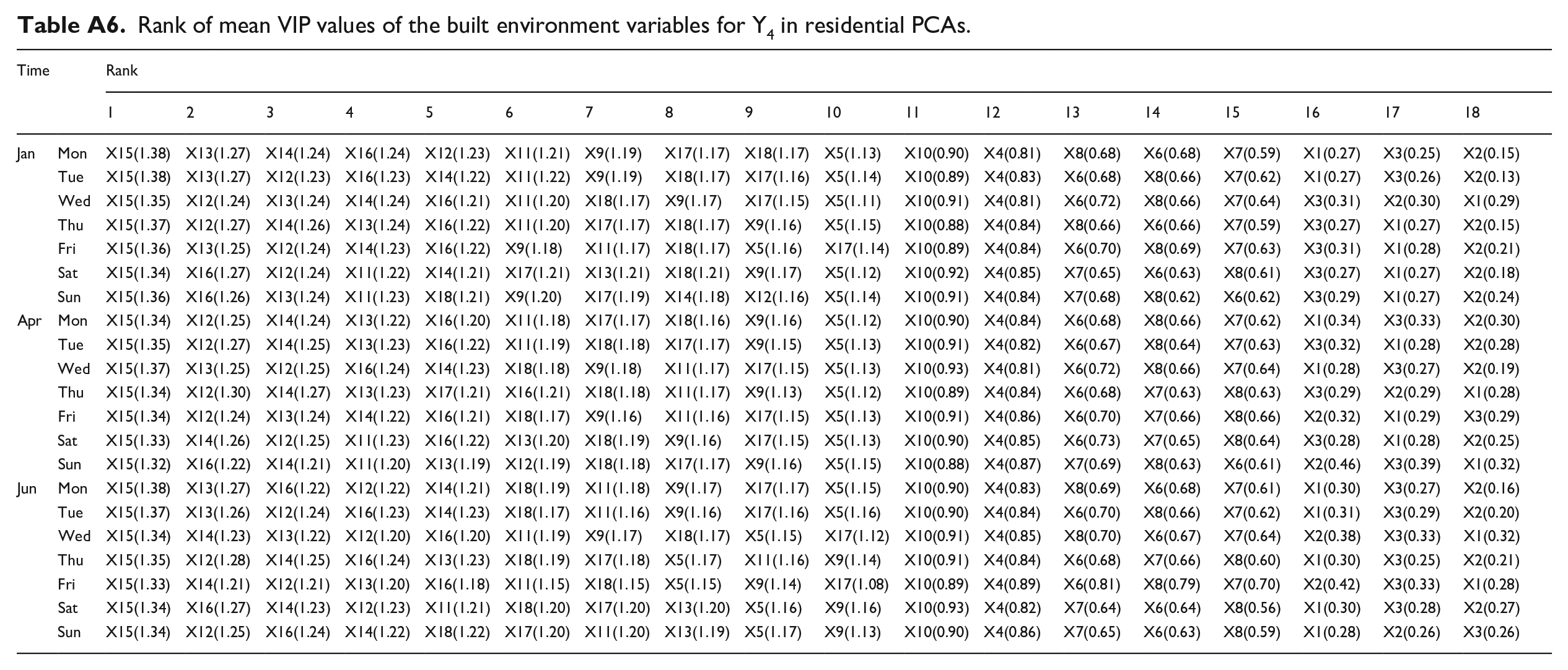
Rank of mean VIP values of the built environment variables for Y₄ in residential PCAs.

Time		Rank
Time		1	2	3	4	5	6	7	8	9	10	11	12	13	14	15	16	17	18
Jan	Mon	X15(1.38)	X13(1.27)	X14(1.24)	X16(1.24)	X12(1.23)	X11(1.21)	X9(1.19)	X17(1.17)	X18(1.17)	X5(1.13)	X10(0.90)	X4(0.81)	X8(0.68)	X6(0.68)	X7(0.59)	X1(0.27)	X3(0.25)	X2(0.15)
	Tue	X15(1.38)	X13(1.27)	X12(1.23)	X16(1.23)	X14(1.22)	X11(1.22)	X9(1.19)	X18(1.17)	X17(1.16)	X5(1.14)	X10(0.89)	X4(0.83)	X6(0.68)	X8(0.66)	X7(0.62)	X1(0.27)	X3(0.26)	X2(0.13)
	Wed	X15(1.35)	X12(1.24)	X13(1.24)	X14(1.24)	X16(1.21)	X11(1.20)	X18(1.17)	X9(1.17)	X17(1.15)	X5(1.11)	X10(0.91)	X4(0.81)	X6(0.72)	X8(0.66)	X7(0.64)	X3(0.31)	X2(0.30)	X1(0.29)
	Thu	X15(1.37)	X12(1.27)	X14(1.26)	X13(1.24)	X16(1.22)	X11(1.20)	X17(1.17)	X18(1.17)	X9(1.16)	X5(1.15)	X10(0.88)	X4(0.84)	X8(0.66)	X6(0.66)	X7(0.59)	X3(0.27)	X1(0.27)	X2(0.15)
	Fri	X15(1.36)	X13(1.25)	X12(1.24)	X14(1.23)	X16(1.22)	X9(1.18)	X11(1.17)	X18(1.17)	X5(1.16)	X17(1.14)	X10(0.89)	X4(0.84)	X6(0.70)	X8(0.69)	X7(0.63)	X3(0.31)	X1(0.28)	X2(0.21)
	Sat	X15(1.34)	X16(1.27)	X12(1.24)	X11(1.22)	X14(1.21)	X17(1.21)	X13(1.21)	X18(1.21)	X9(1.17)	X5(1.12)	X10(0.92)	X4(0.85)	X7(0.65)	X6(0.63)	X8(0.61)	X3(0.27)	X1(0.27)	X2(0.18)
	Sun	X15(1.36)	X16(1.26)	X13(1.24)	X11(1.23)	X18(1.21)	X9(1.20)	X17(1.19)	X14(1.18)	X12(1.16)	X5(1.14)	X10(0.91)	X4(0.84)	X7(0.68)	X8(0.62)	X6(0.62)	X3(0.29)	X1(0.27)	X2(0.24)
Apr	Mon	X15(1.34)	X12(1.25)	X14(1.24)	X13(1.22)	X16(1.20)	X11(1.18)	X17(1.17)	X18(1.16)	X9(1.16)	X5(1.12)	X10(0.90)	X4(0.84)	X6(0.68)	X8(0.66)	X7(0.62)	X1(0.34)	X3(0.33)	X2(0.30)
	Tue	X15(1.35)	X12(1.27)	X14(1.25)	X13(1.23)	X16(1.22)	X11(1.19)	X18(1.18)	X17(1.17)	X9(1.15)	X5(1.13)	X10(0.91)	X4(0.82)	X6(0.67)	X8(0.64)	X7(0.63)	X3(0.32)	X1(0.28)	X2(0.28)
	Wed	X15(1.37)	X13(1.25)	X12(1.25)	X16(1.24)	X14(1.23)	X18(1.18)	X9(1.18)	X11(1.17)	X17(1.15)	X5(1.13)	X10(0.93)	X4(0.81)	X6(0.72)	X8(0.66)	X7(0.64)	X1(0.28)	X3(0.27)	X2(0.19)
	Thu	X15(1.34)	X12(1.30)	X14(1.27)	X13(1.23)	X17(1.21)	X16(1.21)	X18(1.18)	X11(1.17)	X9(1.13)	X5(1.12)	X10(0.89)	X4(0.84)	X6(0.68)	X7(0.63)	X8(0.63)	X3(0.29)	X2(0.29)	X1(0.28)
	Fri	X15(1.34)	X12(1.24)	X13(1.24)	X14(1.22)	X16(1.21)	X18(1.17)	X9(1.16)	X11(1.16)	X17(1.15)	X5(1.13)	X10(0.91)	X4(0.86)	X6(0.70)	X7(0.66)	X8(0.66)	X2(0.32)	X1(0.29)	X3(0.29)
	Sat	X15(1.33)	X14(1.26)	X12(1.25)	X11(1.23)	X16(1.22)	X13(1.20)	X18(1.19)	X9(1.16)	X17(1.15)	X5(1.13)	X10(0.90)	X4(0.85)	X6(0.73)	X7(0.65)	X8(0.64)	X3(0.28)	X1(0.28)	X2(0.25)
	Sun	X15(1.32)	X16(1.22)	X14(1.21)	X11(1.20)	X13(1.19)	X12(1.19)	X18(1.18)	X17(1.17)	X9(1.16)	X5(1.15)	X10(0.88)	X4(0.87)	X7(0.69)	X8(0.63)	X6(0.61)	X2(0.46)	X3(0.39)	X1(0.32)
Jun	Mon	X15(1.38)	X13(1.27)	X16(1.22)	X12(1.22)	X14(1.21)	X18(1.19)	X11(1.18)	X9(1.17)	X17(1.17)	X5(1.15)	X10(0.90)	X4(0.83)	X8(0.69)	X6(0.68)	X7(0.61)	X1(0.30)	X3(0.27)	X2(0.16)
	Tue	X15(1.37)	X13(1.26)	X12(1.24)	X16(1.23)	X14(1.23)	X18(1.17)	X11(1.16)	X9(1.16)	X17(1.16)	X5(1.16)	X10(0.90)	X4(0.84)	X6(0.70)	X8(0.66)	X7(0.62)	X1(0.31)	X3(0.29)	X2(0.20)
	Wed	X15(1.34)	X14(1.23)	X13(1.22)	X12(1.20)	X16(1.20)	X11(1.19)	X9(1.17)	X18(1.17)	X5(1.15)	X17(1.12)	X10(0.91)	X4(0.85)	X8(0.70)	X6(0.67)	X7(0.64)	X2(0.38)	X3(0.33)	X1(0.32)
	Thu	X15(1.35)	X12(1.28)	X14(1.25)	X16(1.24)	X13(1.23)	X18(1.19)	X17(1.18)	X5(1.17)	X11(1.16)	X9(1.14)	X10(0.91)	X4(0.84)	X6(0.68)	X7(0.66)	X8(0.60)	X1(0.30)	X3(0.25)	X2(0.21)
	Fri	X15(1.33)	X14(1.21)	X12(1.21)	X13(1.20)	X16(1.18)	X11(1.15)	X18(1.15)	X5(1.15)	X9(1.14)	X17(1.08)	X10(0.89)	X4(0.89)	X6(0.81)	X8(0.79)	X7(0.70)	X2(0.42)	X3(0.33)	X1(0.28)
	Sat	X15(1.34)	X16(1.27)	X14(1.23)	X12(1.23)	X11(1.21)	X18(1.20)	X17(1.20)	X13(1.20)	X5(1.16)	X9(1.16)	X10(0.93)	X4(0.82)	X7(0.64)	X6(0.64)	X8(0.56)	X1(0.30)	X3(0.28)	X2(0.27)
	Sun	X15(1.34)	X12(1.25)	X16(1.24)	X14(1.22)	X18(1.22)	X17(1.20)	X11(1.20)	X13(1.19)	X5(1.17)	X9(1.13)	X10(0.90)	X4(0.86)	X7(0.65)	X6(0.63)	X8(0.59)	X1(0.28)	X2(0.26)	X3(0.26)

Acknowledgements

The authors are grateful to the two anonymous reviewers for their comments.

Authorship contribution statement

Zhixiang Fang: conceptualization, supervision, methodology, writing – review and editing. Lupan Zhang: data curation, methodology, formal analysis, writing – original draft. Meng Zheng: investigation, validation, writing – review and editing.

Declaration of conflicting interests

The author(s) declared no potential conflicts of interest with respect to the research, authorship, and/or publication of this article.

Funding

The author(s) disclosed receipt of the following financial support for the research, authorship, and/or publication of this article: The research was supported in part by the National Natural Science Foundation of China (Grants 41771473).

Zhixiang Fang is currently a Professor with the State Key Laboratory of Information Engineering in Surveying, Mapping and Remote Sensing, Wuhan University. His research interests include transport geography, big data for human behavior modeling, space-time GIS, and intelligent navigation.

Lupan Zhang is currently a masters student with the State Key Laboratory of Information Engineering in Surveying, Mapping and Remote Sensing, Wuhan University. His research interests include transport geography, smart cities, GIS, and intelligent navigation.

Meng Zheng received the M.E. degree from Wuhan University in 2011. He is currently a Senior Engineer and the Director of Research Department with the Wuhan Transportation Development Strategy Institute. His research interests include tour-based model, traffic simulation, urban spatial analysis, and smart cities.

References

Tong

Liu

Chan

EHW

(2019) Understanding the impact of built environment on metro ridership using open source in Shanghai. Cities 93: 177–187.

Blainey

Mulley

(2013) Using geographically weighted regression to forecast rail demand in the Sydney region. Australasian Transport Research Forum, ATRF 2013 – Proceedings, 1–16.

Bowman

Ben-Akiva

(2001) Activity-based disaggregate travel demand model system with activity schedules. Transportation Research Part A: Policy and Practice 35(1): 1–28.

Cardozo

García-Palomares

Gutiérrez

(2012) Application of geographically weighted regression to the direct forecasting of transit ridership at station-level. Applied Geography 34: 548–558.

Cervero

(2006) Alternative approaches to modeling the travel-demand impacts of smart growth. Journal of the American Planning Association 72(3): 285–295.

Chakour

Eluru

(2016) Examining the influence of stop level infrastructure and built environment on bus ridership in Montreal. Journal of Transport Geography 51: 205–217.

Chakraborty

Mishra

(2013) Land use and transit ridership connections: Implications for state-level planning agencies. Land Use Policy 30(1): 458–469.

Chen

Wang

Zhang

(2019) Discovering the spatio-temporal impacts of built environment on metro ridership using smart card data. Cities 95: 102359.

Chen

Cheng

(2022) What factors influence ridership of station-based bike sharing and free-floating bike sharing at rail transit stations? International Journal of Sustainable Transportation 16(4): 357–373.

10.

Choi

Lee

Kim

Sohn

(2012) An analysis of Metro ridership at the station-to-station level in Seoul. Transportation 39(3): 705–722.

11.

Chu

(2004) Ridership models at the stop level. National Center for Transit Research, Florida Department of Transportation, Report No. BC137-31.

12.

Currie

Ahern

Delbosc

(2011) Exploring the drivers of light rail ridership: An empirical route level analysis of selected Australian, North American and European systems. Transportation 38(3): 545–560.

13.

Ding

Cao

Liu

(2019) How does the station-area built environment influence Metrorail ridership? Using gradient boosting decision trees to identify non-linear thresholds. Journal of Transport Geography 77(April): 70–78.

14.

Fotheringham

Crespo

Yao

(2015) Geographical and Temporal Weighted Regression (GTWR). Geographical Analysis 47(4): 431–452.

15.

Fotheringham

Yang

Kang

(2017) Multiscale Geographically Weighted Regression (MGWR). Annals of the American Association of Geographers 107(6): 1247–1265.

16.

Gan

Yang

Feng

Timmermans

HJP

(2020) Examining the relationship between built environment and metro ridership at station-to-station level. Transportation Research Part D: Transport and Environment 82: 102332.

17.

GOLD

(1998) Creating the Charter of Athens. The Town Planning Review 69(3): 225–247.

18.

Guo

Huang

(2020) Mass Rapid Transit Ridership Forecast Based on Direct Ridership Models: A Case Study in Wuhan, China. Journal of Advanced Transportation 2020: 7538508.

19.

Gutiérrez

Cardozo

García-Palomares

(2011) Transit ridership forecasting at station level: An approach based on distance-decay weighted regression. Journal of Transport Geography 19(6): 1081–1092.

20.

Jun

Choi

Jeong

Kwon

Kim

(2015) Land use characteristics of subway catchment areas and their influence on subway ridership in Seoul. Journal of Transport Geography 48: 30–40.

21.

Kepaptsoglou

Stathopoulos

Karlaftis

(2017) Ridership estimation of a new LRT system: Direct demand model approach. Journal of Transport Geography 58: 146–156.

22.

Kim

Ahn

Choi

Kim

(2016) Sustainable mobility: Longitudinal analysis of built environment on transit ridership. Sustainability 8(10): 1–14.

23.

Kuby

Barranda

Upchurch

(2004) Factors influencing light-rail station boardings in the United States. Transportation Research Part A: Policy and Practice 38(3): 223–247.

24.

Lee

Hong

(2013) Urban structural hierarchy and the relationship between the ridership of the Seoul Metropolitan Subway and the land-use pattern of the station areas. Cities 35: 69–77.

25.

Cai

Jiang

Huang

(2019) Exploring urban taxi ridership and local associated factors using GPS data and geographically weighted regression. Cities 87(129): 68–86.

26.

Lyu

Liu

Tan

Gao

Huang

(2020) The varying patterns of rail transit ridership and their relationships with fine-scale built environment factors: Big data analytics from Guangzhou. Cities 99: 102580.

27.

Lyu

Liu

Yang

(2020) Exploring multi-scale spatial relationship between built environment and public bicycle ridership: A case study in Nanjing. Journal of Transport and Land Use 13(1): 447–467.

28.

Zhang

Ding

Wang

(2018) A geographically and temporally weighted regression model to explore the spatiotemporal influence of built environment on transit ridership. Computers, Environment and Urban Systems 70: 113–124.

29.

Marshall

Grady

(2006) Sketch transit modeling based on 2000 census data. Transportation Research Record 1986(1): 182–189.

30.

McNally

(2007) The Four-Step Model. In Hensher

Button

(eds) Handbook of Transport Modelling. Bingley: Emerald Group Publishing Limited, pp. 35–53.

31.

Mehmood

Liland

Snipen

Sæbø

(2012) A review of variable selection methods in Partial Least Squares Regression. Chemometrics and Intelligent Laboratory Systems 118: 62–69.

32.

Mevik

Wehrens

(2007) The pls package: Principal component and partial least squares regression i R Journal of Statistical Software 18(2): 1–23.

33.

Mukherjee

Sengupta

Sikdar

(2015) Selection of sustainable processes using sustainability footprint method: A case study of methanol production from carbon dioxide. In Fengqi

(ed) Sustainability of Products, Processes and Supply Chains Theory and Applications. Computer Aided Chemical Engineering, Vol. 36. Amsterdam: Elsevier, 311–329.

34.

Ong

Chen

Tsai

Chuang

(2021) Prediction of tea theanine content using near-infrared spectroscopy and flower pollination algorithm. Spectrochimica Acta - Part A: Molecular and Biomolecular Spectroscopy 255: 119657.

35.

Qian

Ukkusuri

(2015) Spatial variation of the urban taxi ridership using GPS data. Applied Geography 59: 31–42.

36.

Qiao

Wang

(2018) A deep belief network with PLSR for nonlinear system modeling. Neural Networks 104: 68–79.

37.

Shiftan

Suhrbier

(2002) The analysis of travel and emission impacts of travel demand management strategies using activity-based models. Transportation 29(2): 145–168.

38.

Sohn

Shim

(2010) Factors generating boardings at Metro stations in the Seoul metropolitan area. Cities 27(5): 358–368.

39.

Sung

Choi

Lee

Cheon

(2014) Exploring the impacts of land use by service coverage and station-level accessibility on rail transit ridership. Journal of Transport Geography 36: 134–140.

40.

Suo

Huang

Zhang

Duan

Shan

(2018) Soil moisture dynamics and dominant controls at di ff erent spatial scales over semiarid and semi-humid areas. Journal of Hydrology 562: 635–647.

41.

Thompson

Brown

Bhattacharya

(2012) What really matters for increasing transit ridership: Understanding the determinants of transit ridership demand in Broward County, Florida. Urban Studies 49(15): 3327–3345.

42.

Cao

Yue

Zhou

(2018) Spatial variations in urban public ridership derived from GPS trajectories and smart card data. Journal of Transport Geography 69(3688): 45–57.

43.

Walters

Cervero

(2003) Forecasting transit demand in a fast growing corridor: the direct-ridership model approach. Fehrs and Peers Associates.

44.

Yan

Liu

Zhao

(2020) Using machine learning for direct demand modeling of ridesourcing services in Chicago. Journal of Transport Geography 83: 102661.

45.

Yang

Fang

Shaw

Zhao

Yin

Zhang

Lin

(2016) Understanding spatiotemporal patterns of human convergence and divergence using mobile phone location data. ISPRS International Journal of Geo-Information 5(10): 177.

46.

Zhang

Wang

(2014) Transit ridership estimation with network Kriging: A case study of Second Avenue Subway, NYC Journal of Transport Geography 41: 107–115.

47.

Zhao

Deng

Song

Zhu

(2013) What influences Metro station ridership in China? Insights from Nanjing. Cities 35: 114–124.

48.

Zhao

Deng

Song

(2014a) Ridership and effectiveness of bikesharing: The effects of urban features and system characteristics on daily use and turnover rate of public bikes in China. Transport Policy 35: 253–264.

49.

Zhao

Deng

Song

Zhu

(2014b) Analysis of Metro ridership at station level and station-to-station level in Nanjing: An approach based on direct demand models. Transportation 41(1): 133–155.

50.

Zhu

Chen

Wang

Deng

(2019) Spatio-temporal analysis of rail station ridership determinants in the built environment. Transportation 46(6): 2269–2289.

Transferability analysis of built environment variables for public transit ridership estimation in Wuhan,China

Abstract

Keywords

Highlights

Introduction

Literature review

Study area and data

Study area

Data description

Methods

Categories of PCAs

Built environment and public transit ridership variables

Regression modeling of the built environment and public transit ridership variables

The importance magnitude of built environment variables

Public transit ridership estimation model and evaluation

Result and discussion

Analyzing the importance magnitude of the built environment variables on regression modeling of the metro and taxi ridership

Analysis of TVs for the metro and taxi ridership

Comparative analysis of the estimation results of the metro and taxi ridership in PCAs

Conclusion

Footnotes

Appendix A

Acknowledgements

Authorship contribution statement

Declaration of conflicting interests

Funding

References