Sage Journals: Discover world-class research

Abstract

This study is intended for researchers (and doctoral students) interested in learning more on the use of machine learning methods in non-investment crowdfunding (i.e., reward- and donation-based). In particular, the study illustrates the insights that machine learning methods could provide on non-investment crowdfunding, for example, through data and information visualization, the ranking of features importance, and prediction assessment metrics. Specifically, I use four machine learning methods (gradient boosted decision trees, random forests, shallow neural networks, and support vector machines). As the literature shows, machine learning methods outperform classical regression models when the underlying relations are nonlinear. As such, the study offers some insights on the nonlinear relationships that could exist between the explanatory variables and the likelihood of success for art projects (e.g., threshold and Goldilocks effects). The study also offers some guidance to art project creators.

Keywords

rewards-based crowdfunding machine learning arts projects threshold effects Goldilocks effects

1. Introduction

This study is intended for researchers and doctoral students interested in learning more on the use of machine learning methods in non-investment crowdfunding (i.e., reward- and donation-based). Crowdfunding has grown tremendously in the last decade as a source of alternative finance. For example, in 2020, $100.86 billion was raised worldwide in debt crowdfunding, US$8.4 B in non-investment crowdfunding, and US$4.41 B in equity crowdfunding (Statista, 2022). At the same time, academic research on crowdfunding has also grown (e.g., Deng et al., 2022; Kaartemo, 2017; Shneor and Vik, 2020; Shneor et al., 2020). The vast majority of studies on non-investment crowdfunding use parametric regression tools (e.g., Molick, 2014; Colombo et al., 2015; Butticè et al., 2017; Bi et al., 2017; Lin and Boh, 2021; Usman et al., 2020; Shneor et al., 2021; Li et al., 2022; Elitzur et al., 2023a)¹. A number of studies use machine learning methods to study noninvestment crowdfunding (Duan et al., 2020, Peng et al., 2021; Elitzur & Solodoha, 2021;²Elitzur, Katz, et al., 2023; Oduro et al., 2022; Wang et al., 2021, 2022; Zhong et al., 2022)^3,⁴. Woods et al. (2020) apply an interesting machine learning model to investigate the spatio-temporal dynamics of successful non-investment crowdfunding campaigns and demonstrate that geography matters, as well as the time of the location. Research shows that machine learning models outperform classical regression models when dealing with nonlinear relationships (Elitzur, Katz, et al., 2023; Liang et al., 2022; Rasekhschaffe and Jones, 2019). Such nonlinear relationships have been demonstrated in the context of non-investment crowdfunding (Elitzur et al., 2023a, 2023b) and, as such, machine learning methods should be better in analyzing them than classical regression models, commonly utilized in crowdfunding research. For example, Elitzur et al. (2023a) show overchoice effects with respect to the number of reward options. Overchoice refers to well documented phenomena where providing a consumer with choice increases participation up to a level where excessive choice occurs and adversely affects participation (Iyengar & Lepper, 2000; Gourville and Soman, 2005; Scheibehenne et al., 2010). As such, overchoice follows a nonlinear function. Elitzur et al. (2023) demonstrate threshold and Goldilocks effects in the context of crowdfunding. Threshold effects lead to changed behavior by backers once a certain threshold is reached (a “tipping point”). Goldilocks effects exist when campaign parameters need to be “just right” for backers to fund a project. Both threshold and Goldilocks effects lead to nonlinear relations between explanatory variables and the likelihood of crowdfunding success. As I demonstrate in this study, because of the nonlinearities in the relationships between explanatory variables and crowdfunding success, we should use machine learning in analyzing crowdfunding as opposed to the commonly used classical regression models.

This study contributes to the literature in four ways. First and foremost, it is provides a teaching tool on the application of machine learning methods in crowdfunding research. Second, the study provides some interesting insights on the nonlinear effects of variables on success for crowdfunding art campaigns (e.g., threshold and Goldilocks effects). Third, the study offers some insights on the effects of non-quantitative variables (specifically, text variables) on the likelihood of success of art projects. Fourth, the database that I created on arts crowdfunding projects, which contains detailed data on 14,612 Kickstarter projects that took place between March 2013 and May 2016, could be explored by researchers (whether using standard parametric regression methods or machine learning tools).

In addition, the study also offers some practical implications to project creators that can be used in the pre-campaign project design, or during the campaign itself, to optimize their likelihood of crowdfunding success.

2. Variables

2.1 General

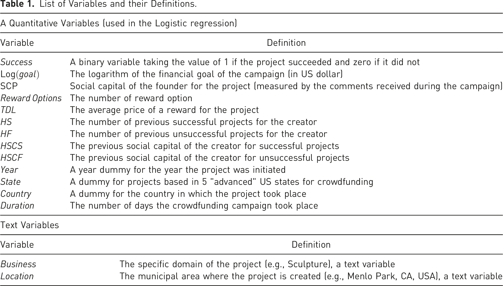
All variables are described in Table 1, where Panel A outlines the numerical data variables (those that can be used in logistic regression). In the first part of the analysis, I will use only these variables to directly demonstrate the advantages of using machine learning methods for nonlinear relationships without adding non-numerical variables⁵. In the second part of the analysis, I will add text variables (outlined in Panel B) to show the value added from the ability of machine learning methods to analyze text variables.

Table 1.

List of Variables and their Definitions.

A Quantitative Variables (used in the Logistic regression)
Variable	Definition
$S u c c e s s$	A binary variable taking the value of 1 if the project succeeded and zero if it did not
$Log (g o a l)$	The logarithm of the financial goal of the campaign (in US dollar)
SCP	Social capital of the founder for the project (measured by the comments received during the campaign)
$R e w a r d O p t i o n s$	The number of reward option
$T D L$	The average price of a reward for the project
$H S$	The number of previous successful projects for the creator
$H F$	The number of previous unsuccessful projects for the creator
$H S C S$	The previous social capital of the creator for successful projects
$H S C F$	The previous social capital of the creator for unsuccessful projects
$Y e a r$	A year dummy for the year the project was initiated
$S t a t e$	A dummy for projects based in 5 "advanced" US states for crowdfunding
Country	A dummy for the country in which the project took place
Duration	The number of days the crowdfunding campaign took place

Text Variables
Variable	Definition
$B u s i n e s s$	The specific domain of the project (e.g., Sculpture), a text variable
$L o c a t i o n$	The municipal area where the project is created (e.g., Menlo Park, CA, USA), a text variable

2.2 Dependent Variable

The dependent variable in our model, Success, is defined (and reported by Kickstarter) as achieving the stated funding goal. Success in Kickstarter is “an all or nothing” proposition (Mollick, 2014) and therefore it is a dichotomous variable, as commonly used in the literature (e.g., Colombo et al., 2015, Josephy et al., 2017; Butticè et al., 2017)⁶ that takes the value of 1 when the campaign is successful and zero when it is not.

2.3 Numerical Independent Variables

Next, I will describe the independent numerical variables and their expected logistic regression coefficients, based on the literature. The effects are more complex for the machine learning methodology because of the embedded nonlinearities and, consequently, do not have necessarily a constant coefficient. Moreover, they can potentially have zero, negative, or positive effects on Success in different regions.

TDL (Threshold Donation Level) is the average price of a Rewards Options (defined below). This variable is expected to have a negative coefficient in a logistic regression model (Elitzur et al., 2023a; Shneor et al., 2021).

SCP (Social Capital of the Project) is the social score of the founder, measured by the comments made on the campaign. We expect this variable to have a positive coefficient in a logistic regression model, i.e., it positively affects the probability of success (Butticè et al., 2017; Colombo et al., 2015; Elitzur et al., 2023a; Usman et al., 2020).

HS and HF are the previous successful campaigns of the creators and their unsuccessful ones, respectively. We expect these variables to have respectively positive and negative coefficients in the logistic regression (Butticè et al., 2017; Usman et al., 2020; Elitzur et al., 2023a).

HSCS and HSCF are the previous creators’ social score for successful campaigns and unsuccessful ones, respectively. We expect these variables to have respectively positive and negative coefficients in the logistic regression (Butticè et al., 2017; Usman et al., 2020; Elitzur et al., 2023a).

Goal is the monetary goal of the campaign. Consistent with the extant literature, we expect this variable to have a negative coefficient in logistic regression, i.e., it negatively affects the probability of success in a logistic regression model (Mollick, 2014; Colombo et al., 2015; Butticè et al., 2017; Bi et al., 2017; Usman et al., 2020; Lin and Boh, 2021; Li et al., 2022). For scaling purposes we will use the logarithm of the goal, Log (Goal).

Duration is the time period during which the campaign was active. Consistent with other studies in this area we expect this variable to have a negative coefficient in a logistic regression model, i.e., this variable negatively affects the probability of success (Mollick, 2014; Bi et al., 2017; Butticè et al., 2017; Colombo et al., 2015; Courtney et al., 2017; Li et al., 2022; Lin and Boh, 2021; Shneor et al., 2021; Skirnevskiy et al., 2017).

Rewards Options is the number of reward options. This variable is expected to have a positive coefficient as it provides more choices to backers. Consistent with the literature, we expect Rewards Options to have a positive coefficient in the logistic regression (Mollick, 2014; Courtney et al., 2017; Kuppuswamy & Bayus, 2017; Lin & Boh, 2021; Mollick, 2014; Shneor et al., 2021).

2.4 Numerical Control Variables

Year is the year of the project launch.

State is dummy variable for projects based in 5 “advanced” US states for crowdfunding (California, Florida, New York, Illinois and Massachusetts).

Country is a dummy variable for the country where the project is created.

2.5 Text Variables (used in the second stage of the machine learning analysis)

Business is the specific domain of the project (e.g., Sculpture).

Location is the municipal area where the project is created (e.g., Menlo Park, California, USA). As Woods et al. (2020) show the location is a major factor in the performance of the campaign.

3. Empirical Setting

3.1 Data Sources

Our data is a subset of the data in Elitzur et al. (2023a, 2023b), using observations on 14,612 art projects. The original dataset contains information about 108,223 projects launched from March 2013 to May 2016. Prior to modeling, the data were randomly partitioned into training, validation, and test sets; we used the standard 50/25/25 partition (Elitzur et al., 2023b, 2023c). The training set, containing 7,306 (50%) observations is used for training the system. It was then used for finetuning the system in the validation sample, which contains 3,653 (25%) observations. Once all parameters are finetuned, the model accuracy is assessed on the test sample (also known as the “holdout sample”), which emulates the expected out-of-sample performance of the model and contains 3,653 (25%) observations. The descriptive statistics and correlation matrix are shown in Table 2 and Table 3, respectively.

Table 2.

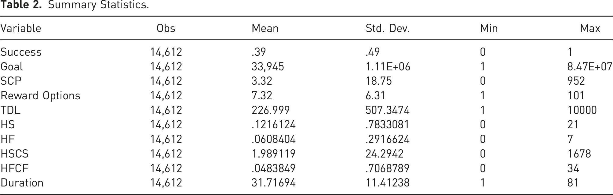
Summary Statistics.

Variable	Obs	Mean	Std. Dev.	Min	Max
Success	14,612	.39	.49	0	1
Goal	14,612	33,945	1.11E+06	1	8.47E+07
SCP	14,612	3.32	18.75	0	952
Reward Options	14,612	7.32	6.31	1	101
TDL	14,612	226.999	507.3474	1	10000
HS	14,612	.1216124	.7833081	0	21
HF	14,612	.0608404	.2916624	0	7
HSCS	14,612	1.989119	24.2942	0	1678
HFCF	14,612	.0483849	.7068789	0	34
Duration	14,612	31.71694	11.41238	1	81

Table 3.

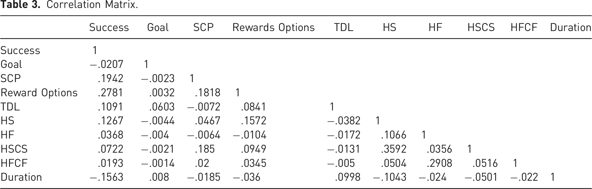
Correlation Matrix.

	Success	Goal	SCP	Rewards Options	TDL	HS	HF	HSCS	HFCF	Duration
Success	1
Goal	−.0207	1
SCP	.1942	−.0023	1
Reward Options	.2781	.0032	.1818	1
TDL	.1091	.0603	−.0072	.0841	1
HS	.1267	−.0044	.0467	.1572	−.0382	1
HF	.0368	−.004	−.0064	−.0104	−.0172	.1066	1
HSCS	.0722	−.0021	.185	.0949	−.0131	.3592	.0356	1
HFCF	.0193	−.0014	.02	.0345	−.005	.0504	.2908	.0516	1
Duration	−.1563	.008	−.0185	−.036	.0998	−.1043	−.024	−.0501	−.022	1

3.2 Regression Equation

The equation for the logistic regression is as follows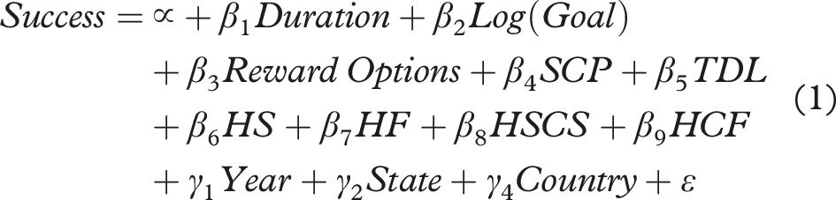

S u c c e s s = \propto + β_{1} D u r a t i o n + β_{2} Log (G o a l) + β_{3} R e w a r d O p t i o n s + β_{4} S C P + β_{5} T D L + β_{6} H S + β_{7} H F + β_{8} H S C S + β_{9} H C F + γ_{1} Y e a r + γ_{2} S t a t e + γ_{4} C o u n t r y + ε

(1)

As discussed in the Variables section, consistent with literature, we expect to have negative coefficients for $D u r a t i o n$ , $Log (G o a l)$ , $T D L$ , $H F$ , $H C F$ and positive coefficients for $S C P$ , $R e w a r d s O p t i o n s$ , $H S$ , and $H S C S$ . equation (1) will be run first for the entire sample and then just for the training dataset.

3.3 Machine Learning Methods

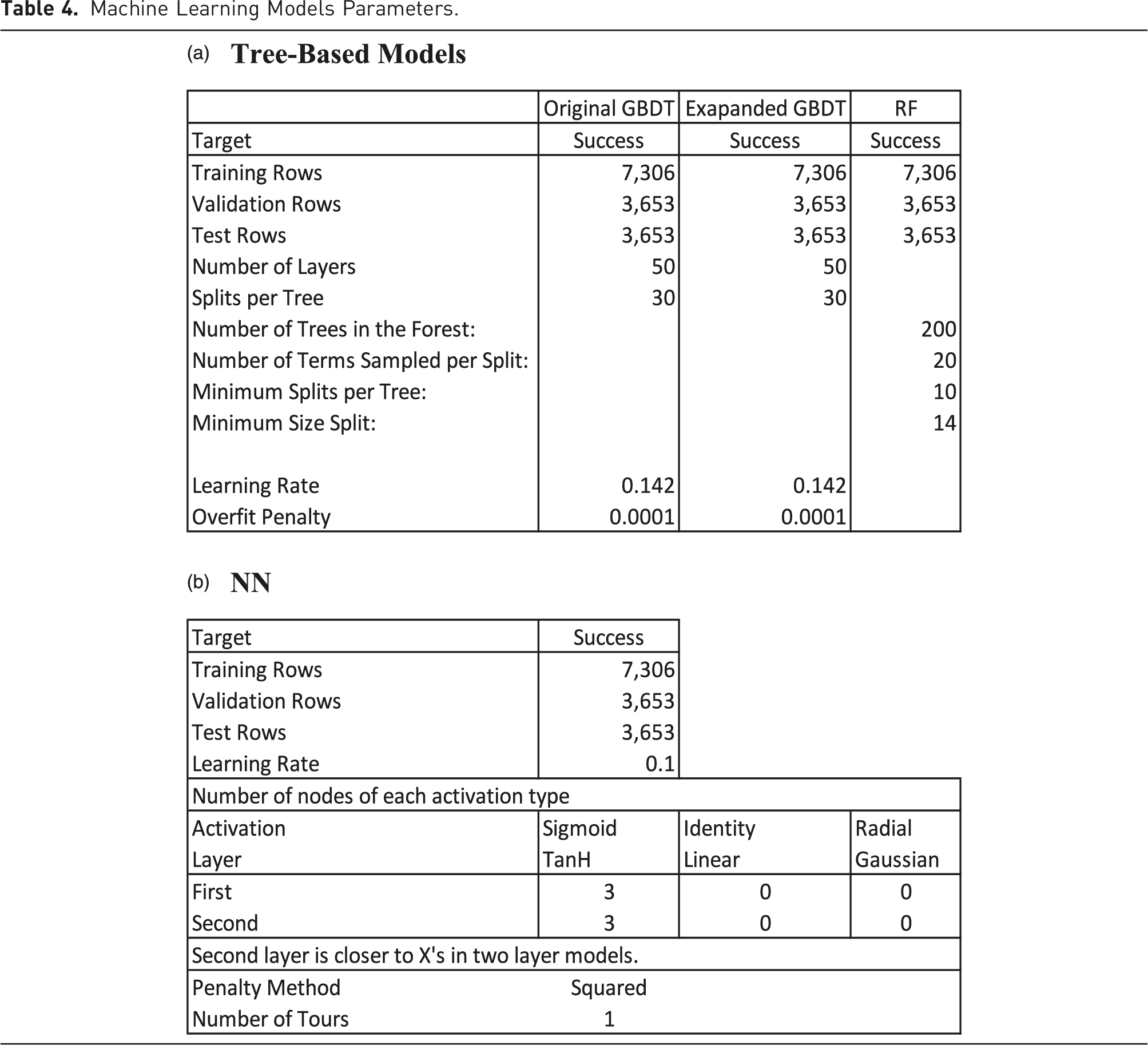
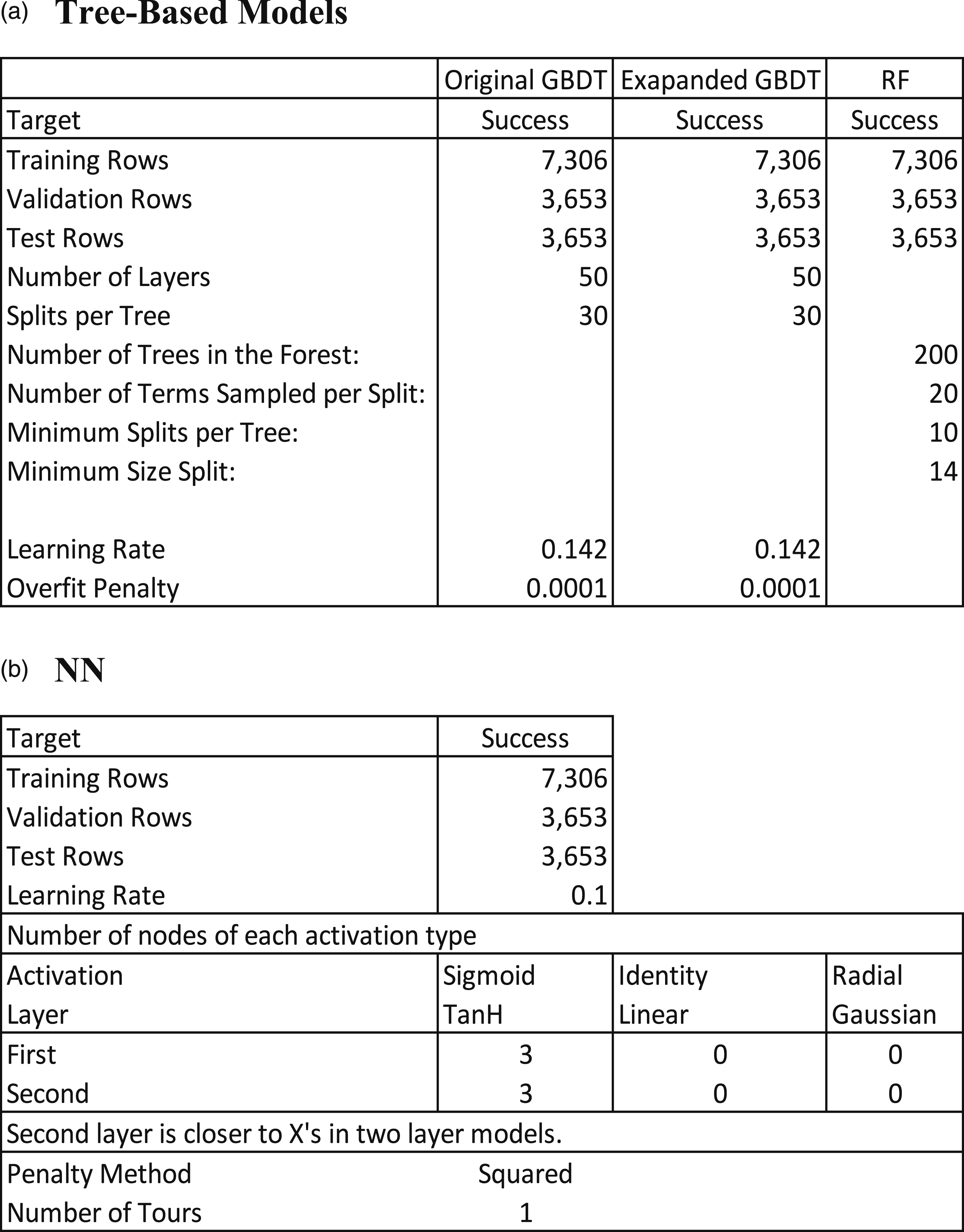
As discussed the Variables section, I will first run the machine learning algorithms using only the same variables used in equation (1) to directly demonstrate the insights added from the nonlinear relations between the independent numerical variables and $S u c c e s s$ . Next, I will add text variables to demonstrate the full potential of these tools.

As discussed in Section 3.1 Data Sources, the sample is randomly partitioned into three datasets: training (7,306 observations, 50%), validation (3,653 observations, 25%), and test (3,653 observations, 25%). It is important to note that the test dataset (also known as holdout sample) contains observations that the system does not access when formulating the model and, as such, it is used to test the predictions of the model created first based on the training dataset and then finetuned based the validation dataset. The machine learning methods that I use include the following:

(1) Gradient Boosted Decision Trees (GBDT)

(2) Random Forests (RF)

(3) Shallow Neural Networks (NN)

(4) Support vector machines (SVM)

These methods, together with Deep Learning are the ones often used in predictive analytics (e.g., Chang et al., 2022; Ma et al., 2018; Zhong et al., 2022). These methods and the theory behind them are discussed at length in Elitzur e al. (2023b, 2023c). The goal of the system is to find the best predictor of success, often referred to as the best classifier, based on the independent variables (often referred to as features in machine learning). Elitzur et al. (2023b) show that Deep Convolutional Neural Networks CNN), a form of Deep Learning, did not provide better prediction than the above methods for their sample. The explanation that they provide is that tree-based machine learning algorithms are better when it comes to tabular data, while Deep Learning approaches perform better on computer vision and natural language processing tasks such as predicting taxi demand or cancer diagnosis (e.g., Liao et al., 2018; Litjens, 2016). The reason for this is that the application of Deep Learning requires a very large sample (millions of observations) to perform better than tree-based algorithms (Najafabadi et al., 2015). The data in Elitzur et al. (2023b) contains tabular data with only 108,223 observations, explaining why tree-based machine learning models performed better than the Deep Learning approach^7,⁸. In this study I use tabular data with even a smaller sample than Elitzur et al. (2023b), 14,612 observations. As a result, I did not apply Deep CNN or other Deep Learning algorithms to this data.

I used JMP^® Pro 17.2.0 (JMP^® Pro) for the machine learning algorithms in this study⁹. The advantage of using JMP® Pro instead of Python scripts is that it is menu driven and provides significant “fire power” as I will discuss in the Results and Discussion sections. Table 4 shows the specifications used in all machine learning models.

Table 4.

Machine Learning Models Parameters.

4. Results

4.1 Regression Models

Table 5 shows the output for the regression models. Model (1) provides the regression output for the full sample while model (2) provides the output for the training dataset only. Note that all the coefficients for both models show the expected signs of the coefficients, except for HSCS (which is not significant). Except for HSCS and HSCF, all other coefficients are either significant at p < .05 (TDL in Model 1) or highly significant at p < .01 (all other coefficients). Note that the McFadden Pseudo R² is the same for both models at .303.

Table 5.

Regression Models.

		All Sample	Training Dataset
Variables	Expected Sign	(1) Success	(2) Success
Duration	−	−.0225*** (−11.02)	−.0207*** (−7.094)
LogGoal	−	−.379*** (−24.90)	−.377*** (−17.50)
Reward Options	+	.0983*** (15.48)	.110*** (13.54)
SCP	+	.452*** (10.26)	.478*** (5.670)
TDL	−	−.000817*** (−9.342)	−.000920*** (−6.873)
HS	+	.407*** (3.399)	.699*** (5.581)
HF	−	.677*** (−6.254)	−.890*** (−5.373)
HSCS	+	−.00962 (−.759)	−.00228 (−.540)
HSCF	−	−.0135 (−.132)	.0295 (.583)
Constant		2.636*** (2.582)	2.671** (2.211)
Observations		14,554	7,236
Wald Chi2		1544	803.2
P		0	0
Log pseudolikelihood		−6769	−3382
McFadden Pseudo R-squared		.303	.303
Country control		Yes	Yes
State control		Yes	Yes

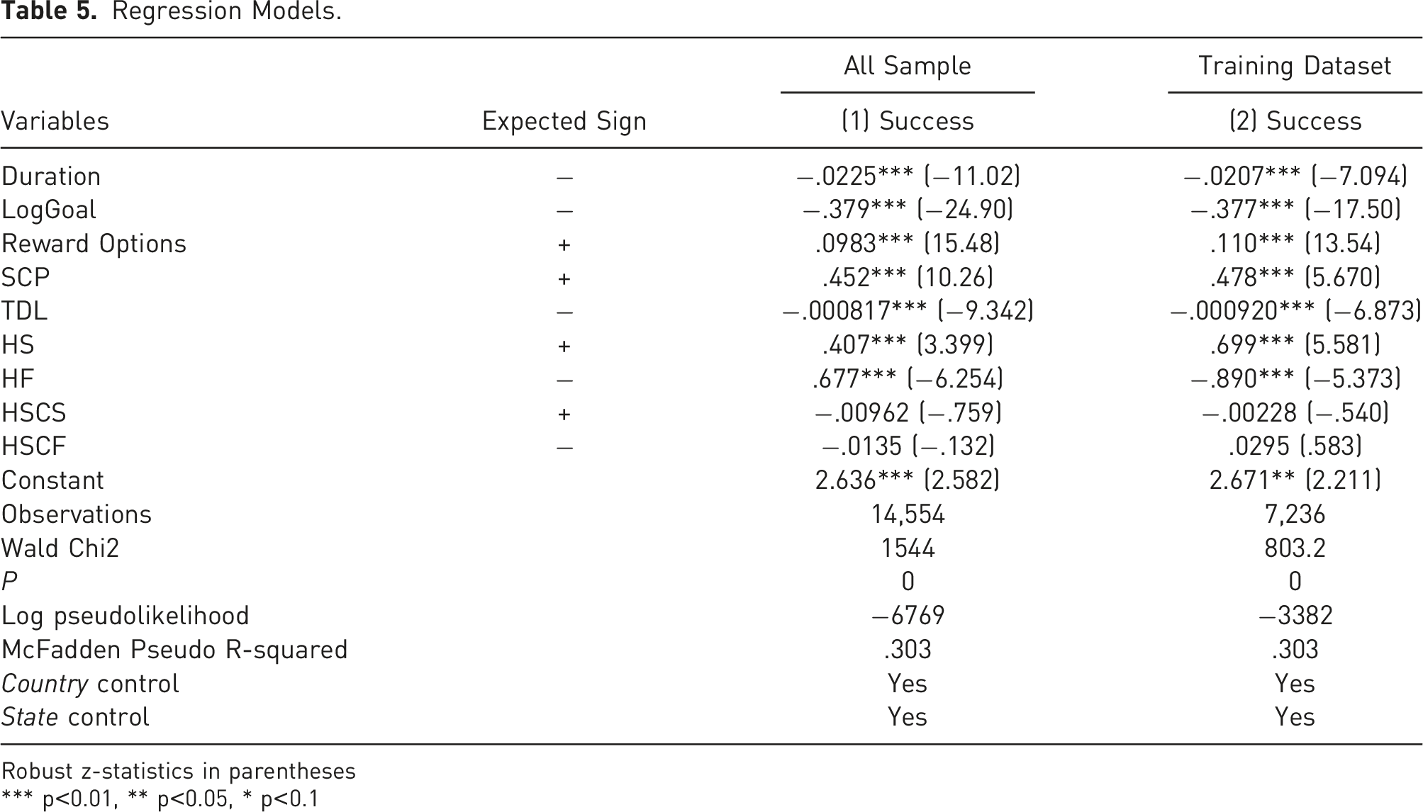
Robust z-statistics in parentheses

*** p<0.01, ** p<0.05, * p<0.1

4.2 Machine Learning Models Results Compared with The Logistic Regression model

One of the commonly used metrics to assess predictive analytics is the Receiver Operating Characteristic (ROC) curve (e.g., Flach et al., 2011, Elitzur e al., 2023b, 2023c). The metric shows the tradeoff between sensitivity (known also as recall, or true positive rate, TPR) and specificity (false positive rate, FPR). The closer the ROC curve to the top-left corner the better is the prediction of the model.

A related metric is the area under the ROC curve (AUC), measuring the aggregated classification performance of both campaign successes and failures (Flach et al., 2011). The highest possible AUC with maximum prediction ability, is 100%.

One of the criteria to assess the quality of prediction is the stability of the ROC curve and the AUC under the three datasets.

Figure 1 demonstrates the stability of the ROC curves and AUC’s under the three datasets, a criterion measuring the quality of prediction. For example, under all datasets the AUC is above 85% for all models. For example, if the AUC for GBDT, the best performing method in the test dataset (the most important one) it is 92.35% in the training set, 87.55% in the validation set and 88.72% in the test set. As expected, the AUC decreases for the test dataset relative to the training set as the predictions of the algorithms are tested on unseen data by them. It is also interesting to observe that the differences among all algorithms in the ROC curves are the largest in the training set (Figure 1(a)), get smaller in the validation dataset (Figure 1(b)) and are the smallest in the test dataset (Figure 1(c)).

Figure 1.

ROC and AUC comparisons. (a) Training dataset, (b) Validation dataset, (c) Validation dataset.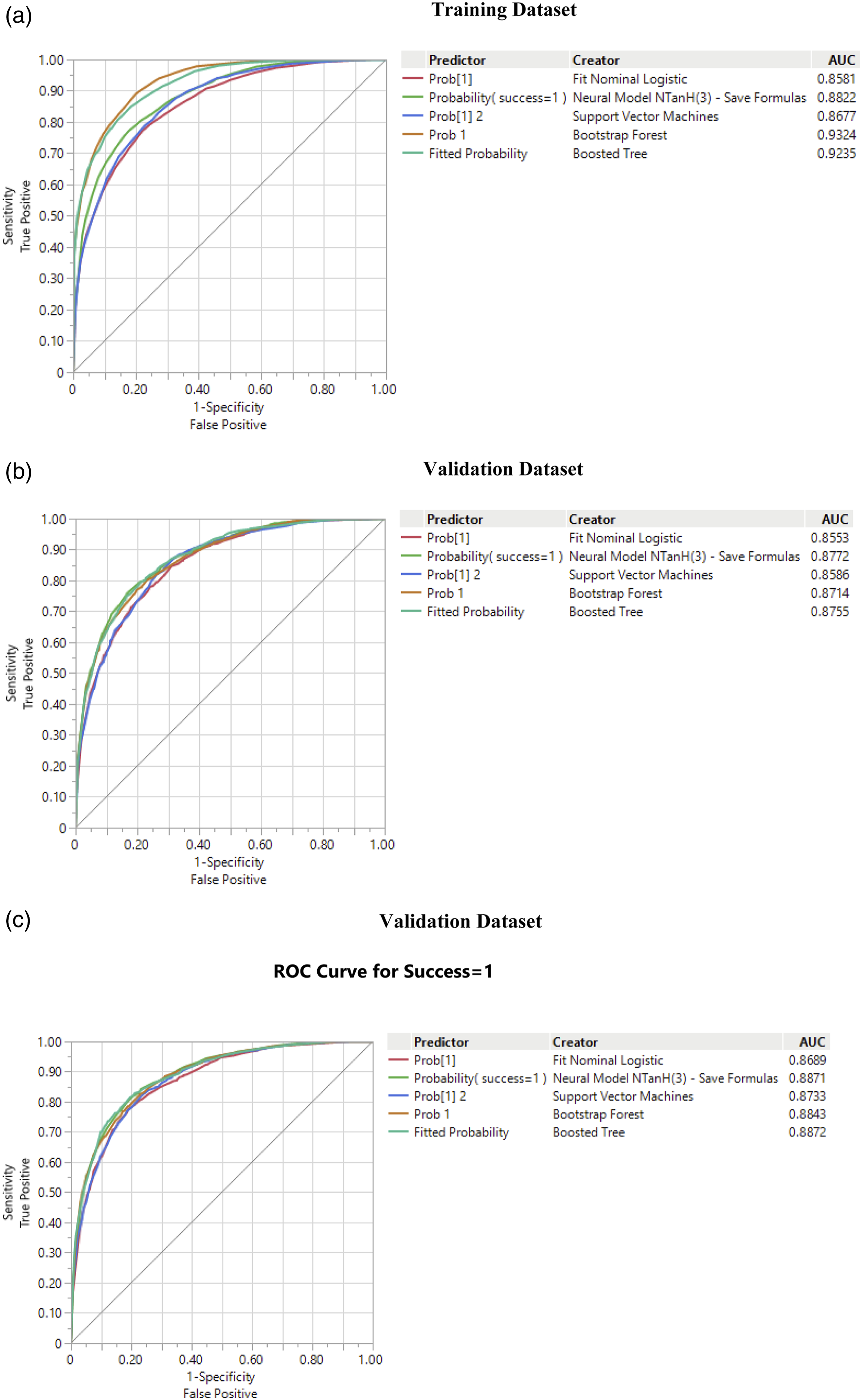

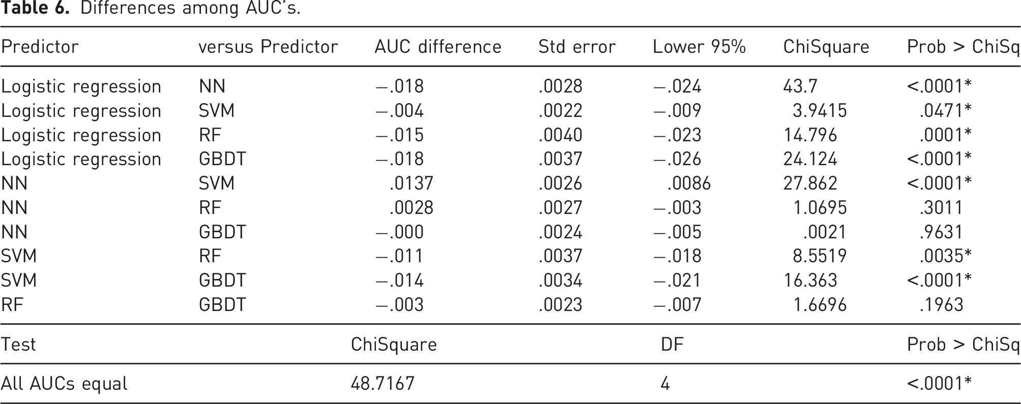
Figure 1(c) demonstrates that the best performing model is the boosted tree (GBDT), which is the closest to the upper left corner and has an AUC of about 88.72%. Next is the shallow neural network with an AUC of about 88.71, followed by Random Forest (RF) model, with an AUC of 88.43%, Support Vector Machines (SVM) with an AUC of 87.33% Last is the logistic regression model with an AUC of about 86.7%.

As Table 6 demonstrates that while all ROC curves seem close, a test that all AUCs are equal shows a 48.72 Chi-Squared statistic for the difference with p < .0001. The Table also shows that the Chi-Squared statistics of the differences among the AUC’s of NN (AUC = 88.71%), RF (AUC of 88.43%) and GBDT however GBDT (AUC = 88.72%) are not significant, implying that the three algorithms are equivalent in terms of prediction. In contrast, SVM’s and the logistic regression’s AUC’s are significantly below those of the GBDT, RF and NN (at p < .05 or p < .01), showing lesser prediction ability.

Table 6.

Differences among AUC’s.

Predictor	versus Predictor	AUC difference	Std error	Lower 95%	ChiSquare	Prob > ChiSq
Logistic regression	NN	−.018	.0028	−.024	43.7	<.0001*
Logistic regression	SVM	−.004	.0022	−.009	3.9415	.0471*
Logistic regression	RF	−.015	.0040	−.023	14.796	.0001*
Logistic regression	GBDT	−.018	.0037	−.026	24.124	<.0001*
NN	SVM	.0137	.0026	.0086	27.862	<.0001*
NN	RF	.0028	.0027	−.003	1.0695	.3011
NN	GBDT	−.000	.0024	−.005	.0021	.9631
SVM	RF	−.011	.0037	−.018	8.5519	.0035*
SVM	GBDT	−.014	.0034	−.021	16.363	<.0001*
RF	GBDT	−.003	.0023	−.007	1.6696	.1963

Test	ChiSquare	DF	Prob > ChiSq
All AUCs equal	48.7167	4	<.0001*

Another means of assessing the performance of prediction models is a confusion matrix. This matrix shows the true positives, false positives, true negatives and false negatives for all prediction models. In our case, it provides the accuracy of prediction with respect to success, failures and the type I and type II errors. As with the ROC curve, the most important matrix is the test dataset one, i.e., the one that shows how well the model performed on out-of-sample data. Table 7 provides the confusion matrices related to all models.

Table 7.

Test Dataset Confusion Matrices.

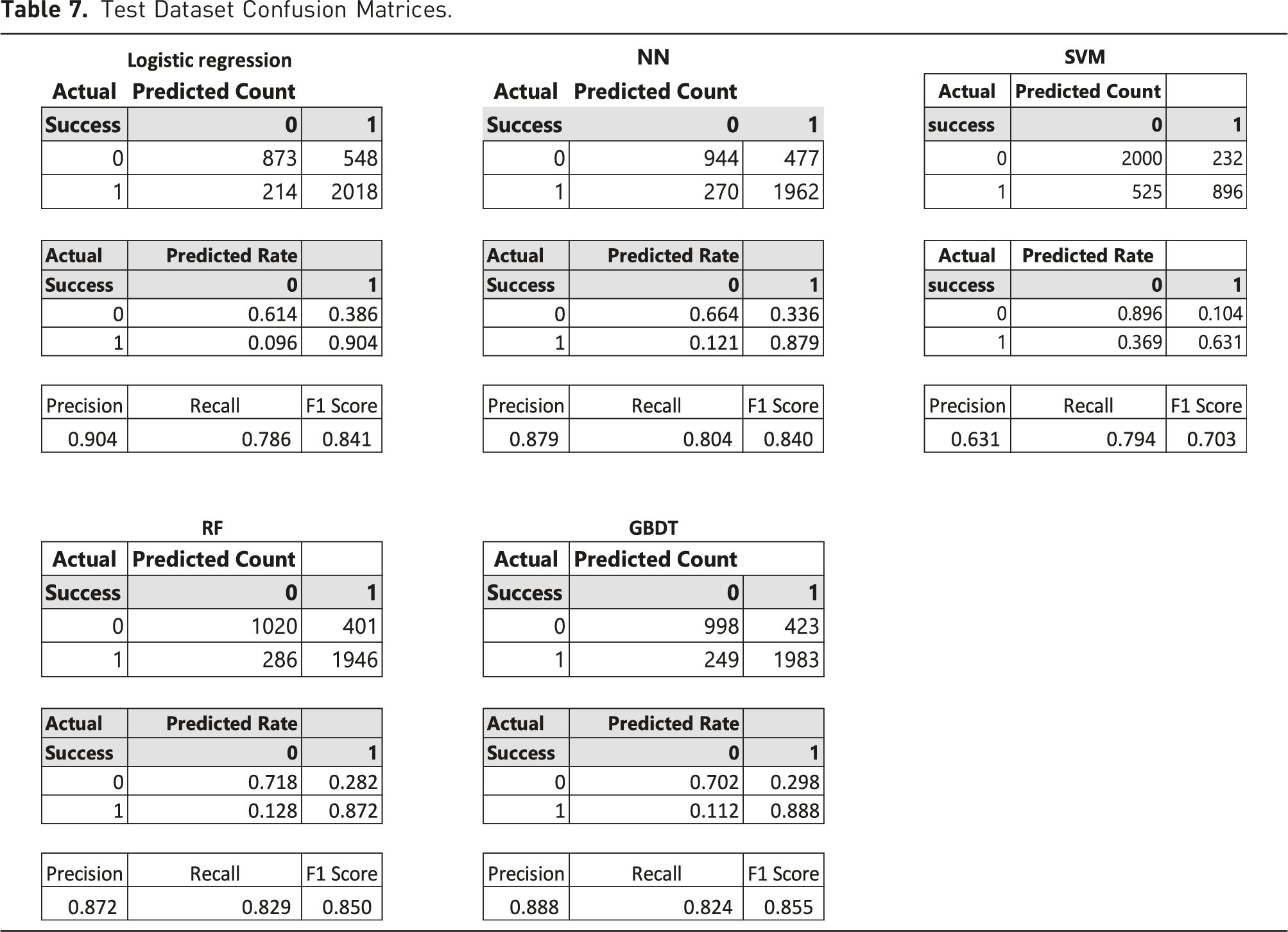
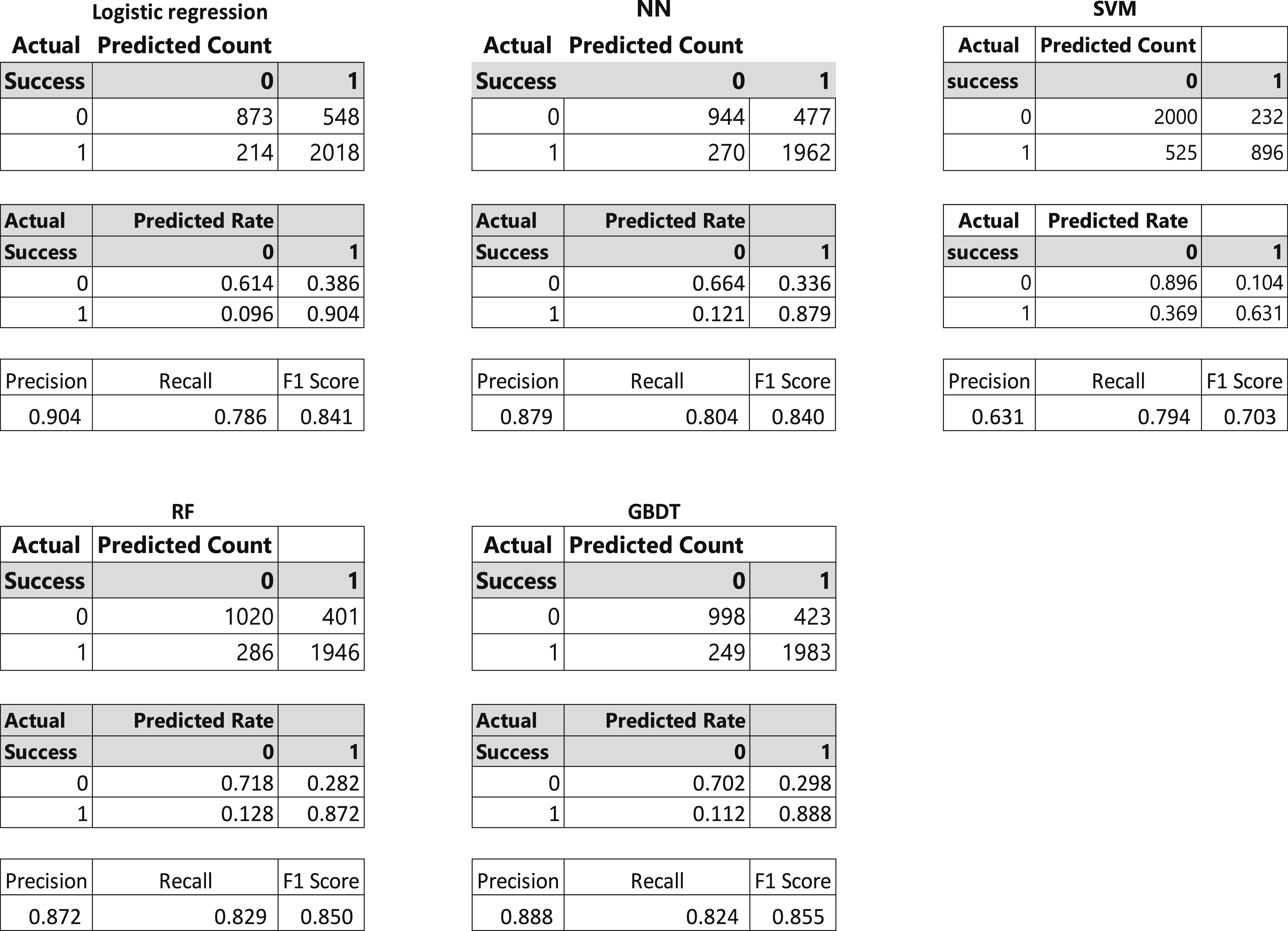
The Table shows that while the logistic regression has the highest precision with respect to predicting success (90%) it also is the worst with the prediction of failure (61%). GBDT performs the best out of the machine learning methods with 89% precision in the prediction of success and 70% in the prediction of failure. Next is NN with 88% precision in the prediction of success and 66% in the prediction of failure, followed by RF with 87% precision in the prediction of success and 72% accuracy in the prediction of failure., and SVM with 63% precision in the prediction of success and 90% in the prediction of failure. The worst performing algorithm is NN with 88% precision in the prediction of success and 66% in the prediction of failure. In terms of recall (sensitivity or true positive rate), RF performs the best (82.9%), followed by GBDT (82.4%), NN (80.4%), SVM (79.4%), and Logistic Regression (78.6%). The F1 Score is an overall measure of prediction quality balancing precision and recall (calculated as $F 1 = 2 X [\frac{P r e c i s i o n X R e c a l l}{P r e c i s i o n + R e c a l l}]$ ). Table 6 shows that GBDT has the highest F1 score (.855), followed by RF (.850), logistic regression (.841), NN (.840), and SVM (.703). As such, the F1 score shows that GBDT is the best performing classifier.

Overall measures of fit are shown in Table 8. The Table demonstrates that the GBDT model performs the best. It has the highest entropy R² (.3884)¹⁰, highest Generalized R² (.5492), lowest Mean-Log p (.4088)¹¹, lowest root average squared error (RASE of .361)¹², the lowest mean absolute deviation (.2638), the best misclassification rate (17.8%, translating to the most accurate prediction rate of 82.2%) and, as previously discussed, the highest AUC (88.72%). As such, all measures of fit demonstrate that GBDT is the best performing classifier.

Table 8.

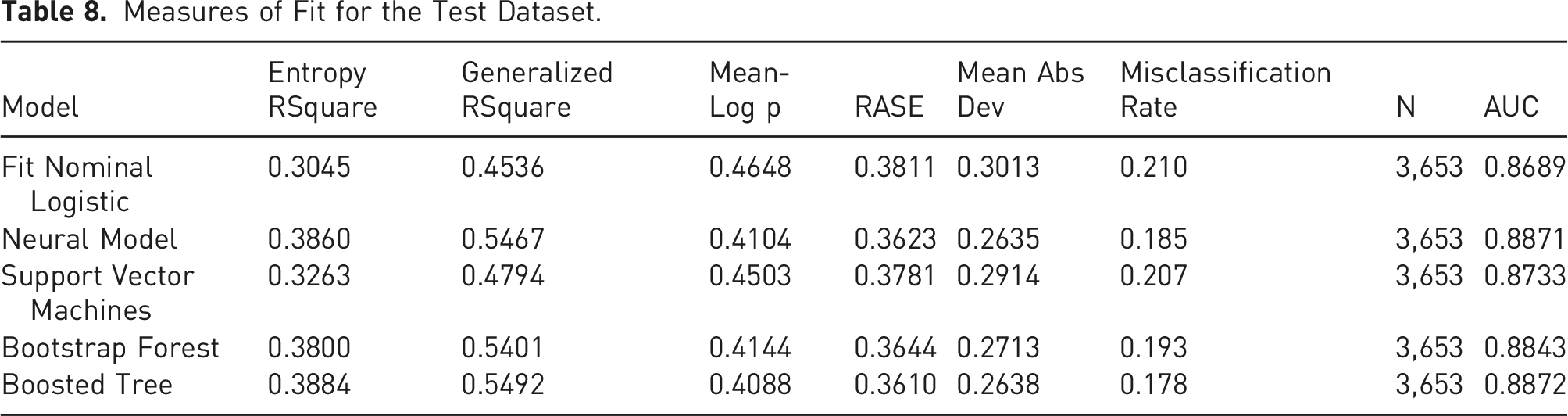
Measures of Fit for the Test Dataset.

Model	Entropy RSquare	Generalized RSquare	Mean-Log p	RASE	Mean Abs Dev	Misclassification Rate	N	AUC
Fit Nominal Logistic	0.3045	0.4536	0.4648	0.3811	0.3013	0.210	3,653	0.8689
Neural Model	0.3860	0.5467	0.4104	0.3623	0.2635	0.185	3,653	0.8871
Support Vector Machines	0.3263	0.4794	0.4503	0.3781	0.2914	0.207	3,653	0.8733
Bootstrap Forest	0.3800	0.5401	0.4144	0.3644	0.2713	0.193	3,653	0.8843
Boosted Tree	0.3884	0.5492	0.4088	0.3610	0.2638	0.178	3,653	0.8872

4.3 Variable Importance

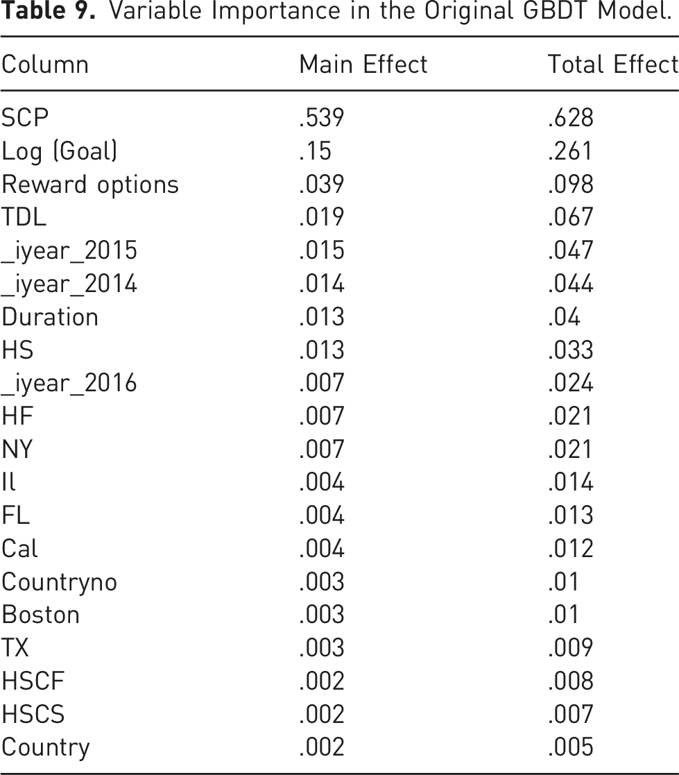
Machine learning provides insights on the effects on the outcome of each variable on its own (main effect) and in interaction with other variables (total effect). It is difficult to assess this effect in regression models as the variable effects relate not just to the size of their coefficients but also to the overall size of variables, as well as their interactions with other variables (which we do not know a priori). In contrast, machine learning models calculate the main and total effects of the variables and, moreover, automatically figure out interaction effects with other variables.

Table 9 ranks variables in order of importance for the best performing algorithm, GBDT, providing both the main and total effects. The importance of social capital of the project creator (SCP) has been demonstrated by Colombo et al. (2015) and Butticè et al. (2017). Refining this, the Table shows that SCP is the most important variable with 54% main effect and 63% total effect. The importance of the goal of the campaign are demonstrated in the extant literature (e.g., Mollick, 2014; Colombo et al., 2015; Butticè et al., 2017; Bi et al., 2017; Usman et al., 2020; Lin & Boh, 2021; Li et al., 2022). As such, the table shows that the Log (Goal) has the second most important effects on the outcome with 15% main effect and 26% total effect. Research demonstrates that the number of Reward Options is important for non-investment crowdfunding success (e.g., Courtney et al., 2017; Kuppuswamy & Bayus, 2017; Lin & Boh, 2021; Mollick, 2014; Mollick, 2014; Shneor et al., 2021). The Table refines this and shows that Rewards Options is the third most important variable for the success of art projects campaigns (4% main effect and 10% total effect). Shneor et al. (2021) and Elitzur et al. (2023b) show the importance of Threshold Donation Level (TDL). Refining this, the Table show that TDL affects the outcome with 2% main effect and 6.7% total effect. Next, we find the year of the project, Duration and HS. All other variables have less than 1% main effect¹³.

Table 9.

Variable Importance in the Original GBDT Model.

Column	Main Effect	Total Effect
SCP	.539	.628
Log (Goal)	.15	.261
Reward options	.039	.098
TDL	.019	.067
_iyear_2015	.015	.047
_iyear_2014	.014	.044
Duration	.013	.04
HS	.013	.033
_iyear_2016	.007	.024
HF	.007	.021
NY	.007	.021
Il	.004	.014
FL	.004	.013
Cal	.004	.012
Countryno	.003	.01
Boston	.003	.01
TX	.003	.009
HSCF	.002	.008
HSCS	.002	.007
Country	.002	.005

4.4 Visualization

As I previously discussed, machine learning algorithms are more effective than regression models in analyzing nonlinear relationships (e.g., Elitzur et al., 2023b). Consequently, visualization of the effects of the explanatory variables on the outcome could provide invaluable insights. For example, Elitzur et al. (2023b) demonstrate the presence of threshold and Goldilocks effects with respect to the full Kickstarter sample. Figures 2(a)-2(d) show the prediction profiler for the 4 most important variables when they are changed while the others are held constant. As such, the Figure depicts the effects of SCP, Log (Goal), Rewards Options and TDL on the likelihood of success for the best classifier, GBDT. The vertical axis is the probability of success, and the horizontal axis is the level of the explanatory variable plotted.

Figure 2.

Prediction profiler for the GBDT model. (a) SCP effects, (b) Log (Goal) effects, (c) Reward options effects, (d) TDL effects.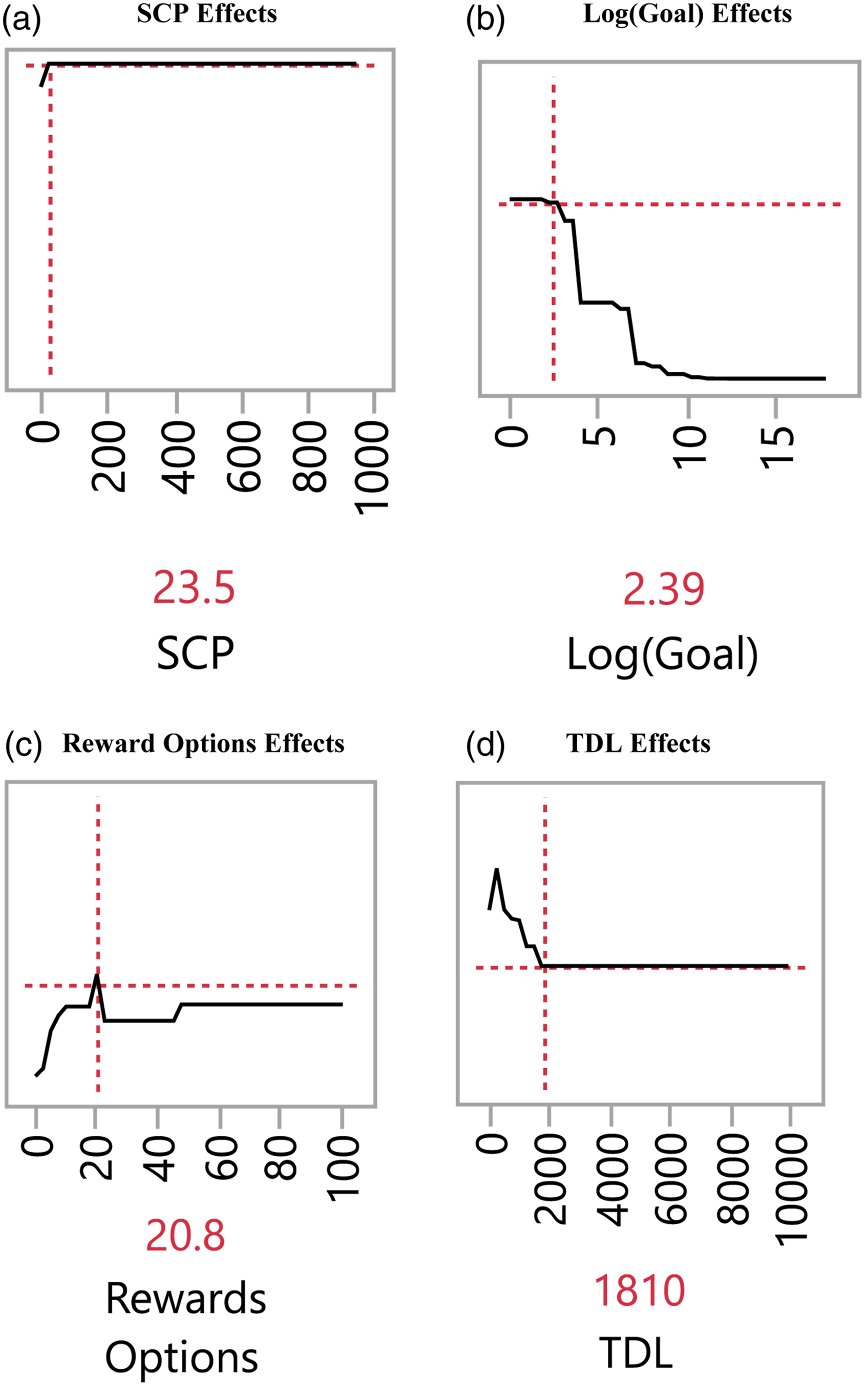

Figure 2(a) depicts the effects of SCP on the likelihood of success for art projects. It shows a threshold (tipping points) at SCP of 23.5. Note that the effects of SCP do not show a constant positive slope simplistic as the logistic regression and the literature predict (e.g., Butticè et al., 2017; Colombo et al., 2015; Usman et al., 2020).

Figure 2(b) demonstrates multiple threshold effects of the goal of the campaign (Log (Goal)) on the likelihood of success for art projects, taking a 3-step function shape. For example, the effect is flat until a threshold at Log (Goal) of 2.39 (translating to campaign goal of US$245.5). The effect then between Log (Goal) of 2.39 (US$245.5) and 3.36 (US$2,291) becomes moderately negative, followed by a negative effect with a steep slope, between Log (Goal) of 3.36 (US$2,291) and 4.53 (US$33,884), followed again by a flat region. This of course contradicts the logistic regression model’s, simplistic prediction of a constant negative positive slope. This also provides a refinement to the extant literature’s simplistic prediction of a constant negative positive slope (Mollick, 2014; Colombo et al., 2015; Butticè et al., 2017; Bi et al., 2017; Usman et al., 2020; Lin and Boh, 2021; Li et al., 2022), Figure 2(c) demonstrates the effect of the number of Reward Options on the likelihood of success for art projects. The Figure shows, consistent with Elitzur et al. (2023a), overchoice effects. Specifically, the likelihood of success increases up to a Goldilocks number of options, 21, beyond which the likelihood of success decreases. These nonlinear (threshold and Goldilocks effects) effects are in contrast with the simplistic predictions of a constant positive slope from the logistic regression, and the extant literature (Mollick, 2014; Courtney et al., 2017; Kuppuswamy & Bayus, 2017; Lin and Boh, 2021; Mollick, 2014; Shneor et al., 2021).

Figure 2(d) graphs the effects of TDL (the average price of a reward option). The Figure shows that up to a threshold TDL of US$270 the likelihood of success for an art campaign increases in TDL, then it declines up to a TDL of US$1,810 and then flattens out. The figure demonstrates a Goldilocks effect at 21, where the TDL is “just right”. These nonlinear (threshold and Goldilocks effects) effects are in contrast with the simplistic prediction of the logistic regression model (and the literature’s, e.g., Shneor et al., 2021) of a constant negative slope.

4.5 Decision Trees Graphs

In contrast with NN or Deep Learning where we cannot visualize prediction drivers, tree-based algorithms (GBDT and RF) can provide the decision trees leading to predictions. The ability to look at trees, branches, and leaves provides intuition on how the system structured trees and, moreover, provides a means to audit the models, and revise them if needed.

Depicting forests for RF or all trees for GBDT is impractical. For example, As Table 4 shows, our GBDT model has 50 layers, with 30 splits each, which would make it impossible to look at all of them at once. Moreover, even showing a whole tree is impractical (due to 30 splits in each tree). We can however look at segments of the trees. As an example, Figure 3 shows a branch and leaves from layer 30 of the model.

Figure 3.

A branch and leaves from layer 30.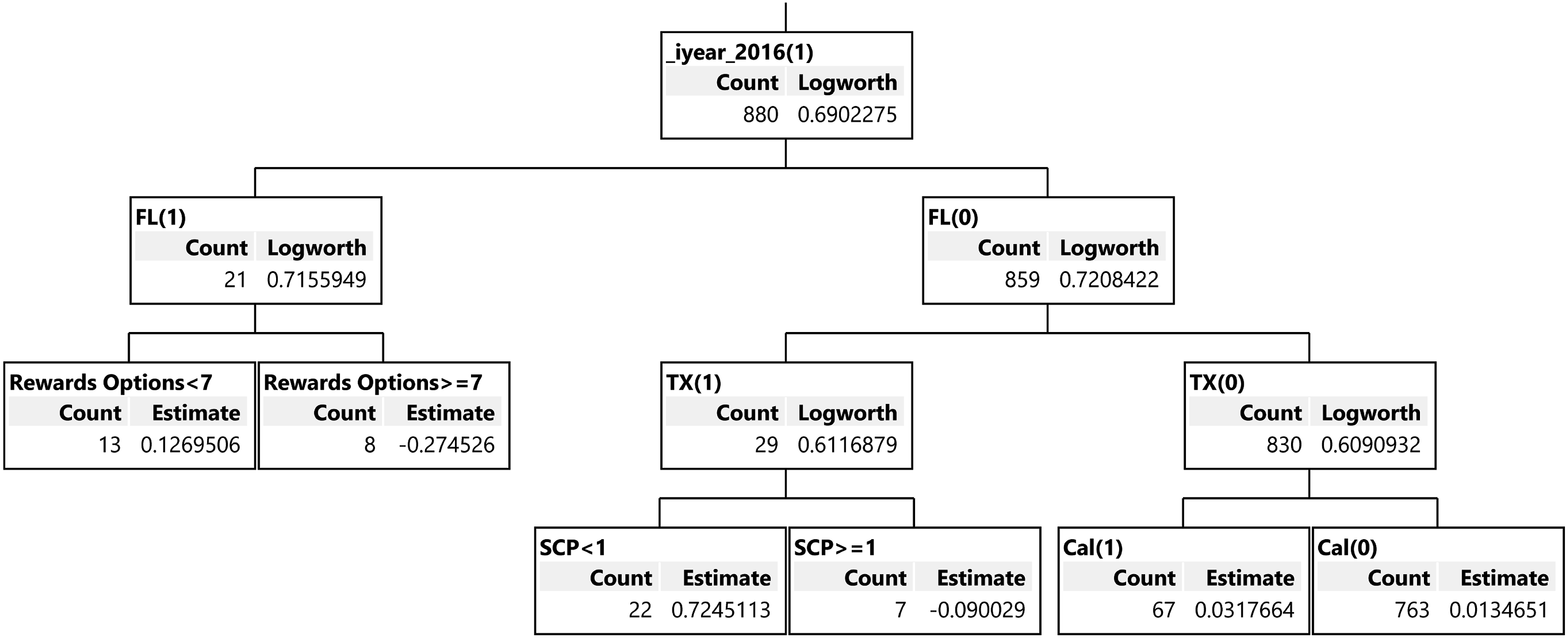

The top branch in Figure 3 shows projects from 2016 (denoted as _iyear_2016 (1)). On the second level it splits into those from Florida (left branch, denoted as FL (1)) and those outside of Florida (right branch, denoted as FL(O)). On the third level Florida projects, FL (1), are split into those with less than 7 rewards options (the leaf on the left, denoted as Rewards Options <7) and those with at least 7 reward options (the leaf on the right, denoted as Rewards Options >=7). Also, on the third level the non-Florida projects, FL (0),are split into those from outside of Texas (the leaf most to the right, denoted as TX (0)) and those from Texas (the next leaf on the left, Denoted as TX (1)). On the fourth level, the non-Texas projects, TX (0), are split into those outside of California (the leaf most to right, denoted as Cal(0)) and those from California (the next leaf to the left, denoted as Cal(1)). The Texas projects on the fourth level, TX (1), are split into projects without any SCP (the left leaf, denoted as SCP <1) and those with some SCP (the right leaf, denoted as SCP >=1).

4.6 Robustness Tests

The procedures that I used for machine learning models have some automatically built-in robustness tests. First, the random partitioning into the three sets where the system learns and finetunes itself (the training and validation datasets, respectively) and then evaluates the performance of its predictions on a dataset that the system did not previously access (the test dataset) is a robustness test to ascertain that the results are not spurious.

Second, running four alterative predictive analytics models and comparing them (logistic regression, GBDT, RF, SVM, and NN) offers another robustness test, ruling out that the results are not driven by some idiosyncratic methodological aspects of the model.

Third, I ran 5-Fold cross-validation as another means to validate the data. The advantage of K-Fold cross-validation analysis is it does not partition the data into three subsets but instead resamples the data, therefore in contrast with the training/validation/test dataset, it maintains the sample size (Shalev-Shwartz and Ben-David, 2014). The main disadvantage of K-Fold cross validation is its problem with external validity (MAQC Consortium, 2010; Rao & Fung, 2008; ) and, as such, it is used here as a robustness test rather than the main approach. The lack of external validity stems from the fact that K-Fold cross-validation is a resampling technique that uses different iterations on various parts of the data for training an algorithm and validating it. In contrast, our main approach uses a dataset, which was never seen by the algorithm, to maximize external validity¹⁴. Appendix A provides the output of the 5-Fold technique. Appendix A Panel A shows that the NN has the highest AUC (.8819). Appendix A Panel B shows that the AUC for the NN algorithm is significantly better than all other methods (at p < .01). This AUC however is worse than the under the three-set (.8872 for the GBDT and .8871 for NN). Moreover, Appendix A Panel D shows that the three-set validation method is better for all algorithms for precision, recall and the F-1score. As such, the three-set validation method (training/validation/test) provides better prediction ability than the 5-Fold validation method.

5. Expanding the Model to Include Text Variables

5.1 Text Variables Added

As discussed in the variable section the data contains two text variables that can add some insights and further prediction power: Business and Location. The analysis in this part uses GBDT, the best performing machine learning method, and assesses it with the metrics that were discussed in the Results section. As I show next, the expanded model (the one with the added text variables) significantly outperforms the original model in its predictions involving the test dataset.

5.2 ROC Curve Comparison

Figure 4 compares the ROC curves for the test dataset of the original model (in red) and the expanded model (the one with the added text variables) in blue. The Figure demonstrates that the expanded model clearly outperforms the original model, as the ROC curve for the expanded model is closer to the upper left corner than the original model.

Figure 4.

ROC comparison between GBDT models. (a) ROC curve, (b) AUC comparison.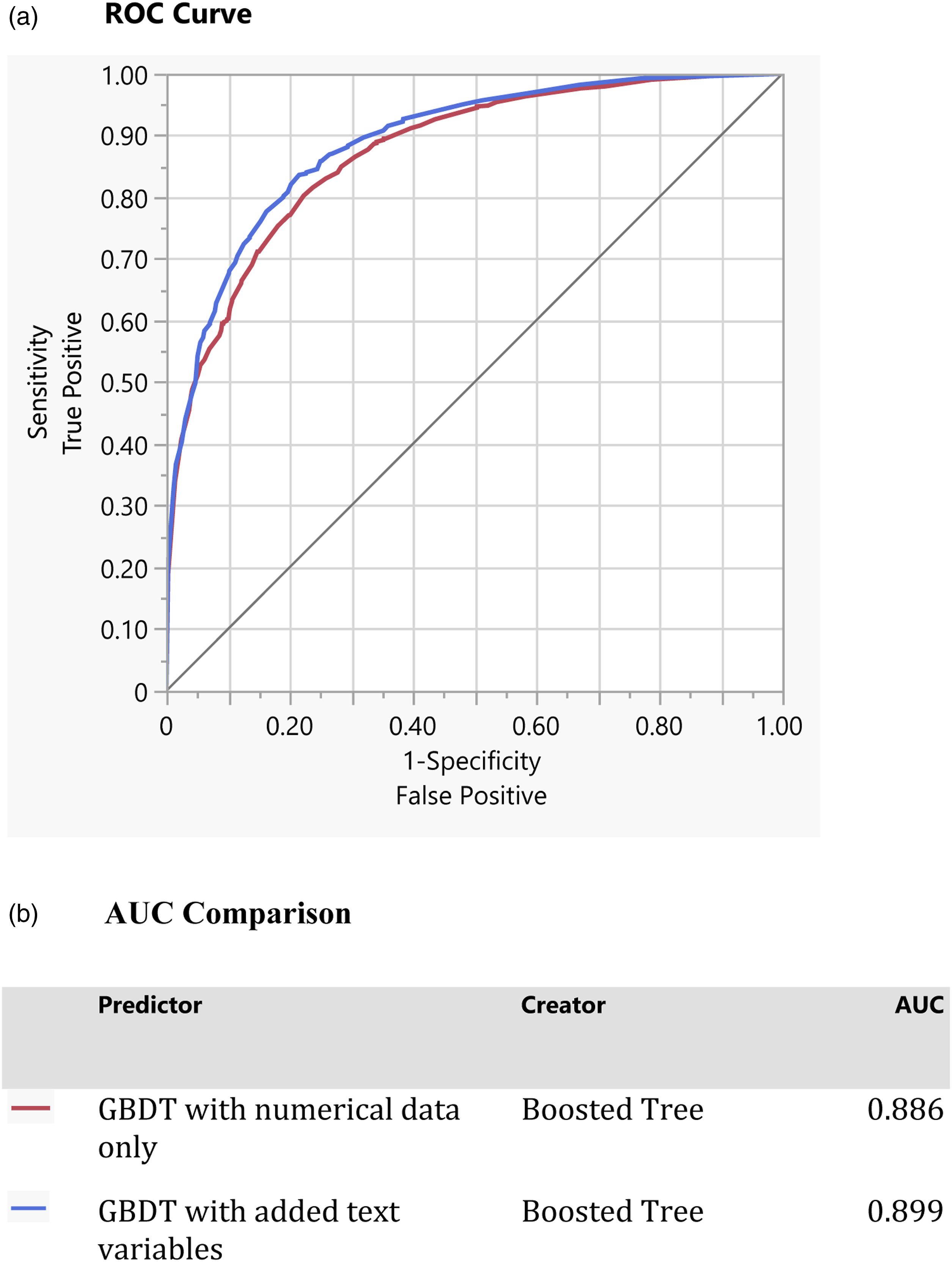

5.3 Performance Metrics Comparison

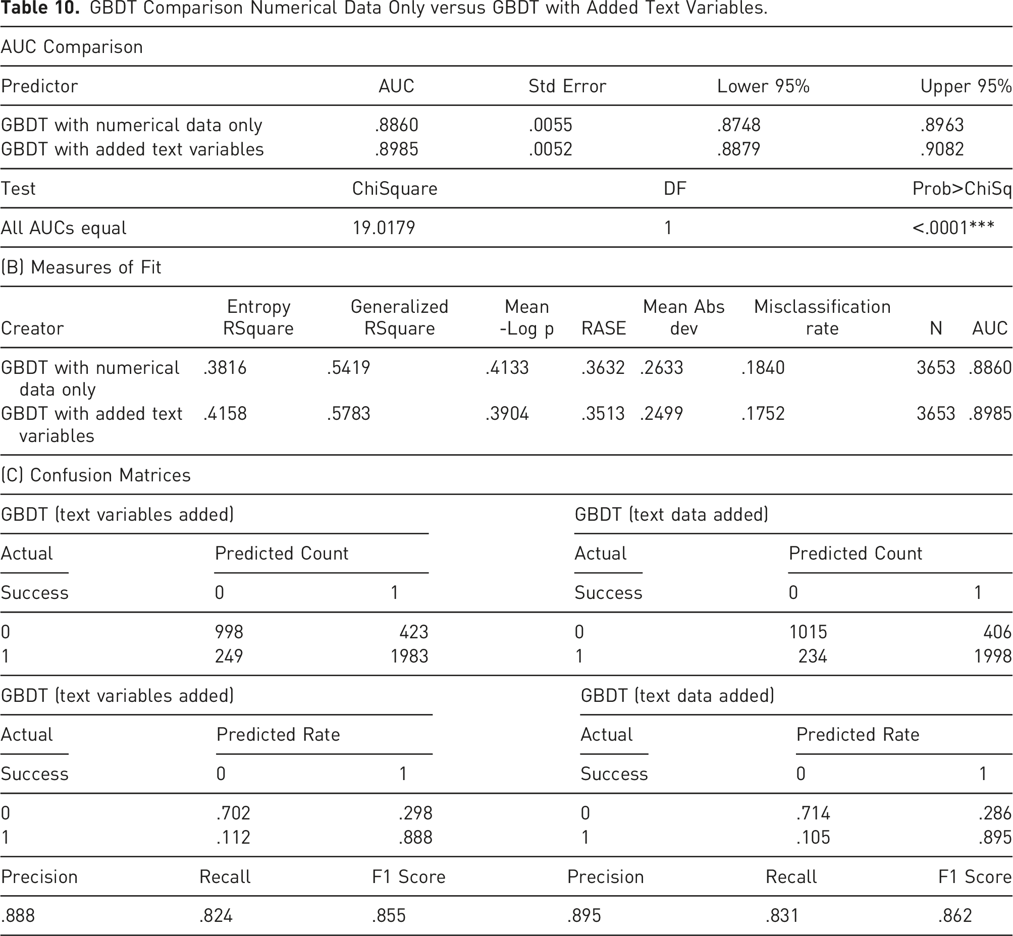
Table 9 Panel A compares the AUC of the original and expended GBDT models. It demonstrates the advantage of the expanded model by showing that the AUC for the expanded model (.899) is higher than the original model’s (.886). Table 9 Panel A shows that the difference between the two ROC curves is highly significant, having a Chi-Squared statistic of 19.02 with p < .0001.

Panel B in Table 9 demonstrates that the expanded model outperforms the original model in any measure of fit for the test dataset. It has a higher Entropy R² (41.6% vs. 38.2%), a higher Generalized R² (58% vs. 54%), a lower Mean-Log p (.39 vs. .41), a lower RASE (.35 vs. .36), a lower Mean Abs Dev (.25 vs. .26), a lower misclassification rate (17.5% vs. 18.4%), and as previously pointed out a significantly higher AUC (.899 vs. .866).

Panel C in Table 9 shows the confusion matrix for the test dataset. It demonstrates that the expanded model is more precise in both predicting success (.895 vs. .888) and failure (.714 vs. .702). Moreover, the expanded model outperforms the original model in precision (.895 vs. .888), recall (.831 vs. .824), and F1 Score (.862 vs. .855).

5.4 Importance of Variables Comparison

Table 10 shows the ranking of the variables under the expanded model versus the original model. The Table shows that both added text variables ae important. Business ranks as the third most important variable, having 8.1% main effect and 12.8 total effect. Consistent with Woods et al. (2020), Location ranks as the 11^th most important variable with 1% main effect and 2.4% total effect. The Table demonstrates that the most important variables from the original model are still important under the expanded model. For example, SCP and Log (Goal) are still respectively the most important and second most important variables, however with smaller effects than the original model.

Table 10.

GBDT Comparison Numerical Data Only versus GBDT with Added Text Variables.

AUC Comparison
Predictor	AUC	Std Error	Lower 95%	Upper 95%
GBDT with numerical data only	.8860	.0055	.8748	.8963
GBDT with added text variables	.8985	.0052	.8879	.9082

Test	ChiSquare	DF	Prob>ChiSq
All AUCs equal	19.0179	1	<.0001***

(B) Measures of Fit
Creator	Entropy RSquare	Generalized RSquare	Mean -Log p	RASE	Mean Abs dev	Misclassification rate	N	AUC
GBDT with numerical data only	.3816	.5419	.4133	.3632	.2633	.1840	3653	.8860
GBDT with added text variables	.4158	.5783	.3904	.3513	.2499	.1752	3653	.8985

(C) Confusion Matrices
GBDT (text variables added)			GBDT (text data added)
Actual	Predicted Count		Actual	Predicted Count
Success	0	1	Success	0	1
0	998	423	0	1015	406
1	249	1983	1	234	1998

GBDT (text variables added)			GBDT (text data added)
Actual	Predicted Rate		Actual	Predicted Rate
Success	0	1	Success	0	1
0	.702	.298	0	.714	.286
1	.112	.888	1	.105	.895

Precision	Recall	F1 Score	Precision	Recall	F1 Score
.888	.824	.855	.895	.831	.862

5.5 Visualization of the Added Text Variables

Figure 5 shows the Prediction Profiler for Business.¹⁵ Figure 5(a) shows that the highest likelihood of success occurs when the stated business is nonspecific (art). Figures 5(b) and 5(c) show, respectively, that the two domains with the next highest likelihood of success are Installation and Performance Art. Figure 5(d) demonstrates that do-it-yourself (DIY) projects have the lowest likelihood of success. In summary, the Figure shows that beyond the project category, which has been shown to be important in the literature (e.g., Mollick, 2014; Buttice` et al., 2017; Colombo et al., 2015) the domain of the project could profoundly affect the likelihood of success.

Figure 5.

Prediction profiler for business in the expanded GBDT Model. (a) Generic description, (b) Installation, (c) Perf. Arts FIGURE 5D - DIY.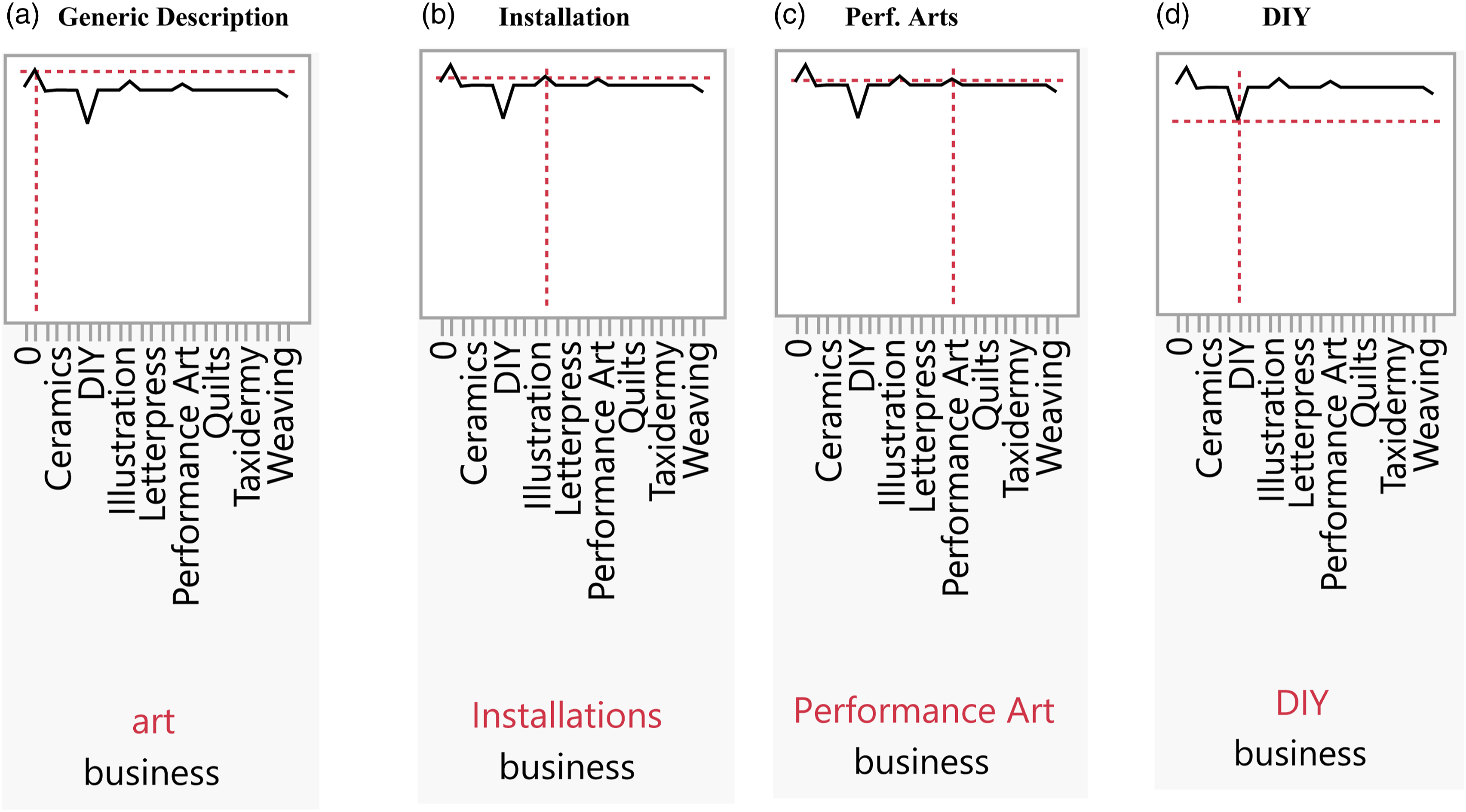

6. Discussion

6.1 Contribution to the Academic Literature

Table 11 The study is meant to be teaching tool and, as such, provides a structured guidance on machine learning methods in the context of non-investment crowdfunding. It purports to help researchers and doctoral students better understand machine learning models and related best practices. The study also offers some notion of the insights that machine learning can impart. For example, the study gives details of the conditions under which machine learning tools outperform the commonly used regression models (namely, when there are nonlinear effects of the explanatory variables on the outcome). In addition, this study provides some guidance on the prevention of overfitting, which entails random partitioning of the data into three datasets: training, validation, and test. It also explains and illustrates the tools that should be used to assess the output from these models (e.g., ROC curves, AUC, measures of fit and confusion matrices). It also illustrates the ranking of variables in terms of their impact on the outcome (on their own and in interaction with other variables). In addition, the study offers some interesting insights on data and information visualization.

Table 11.

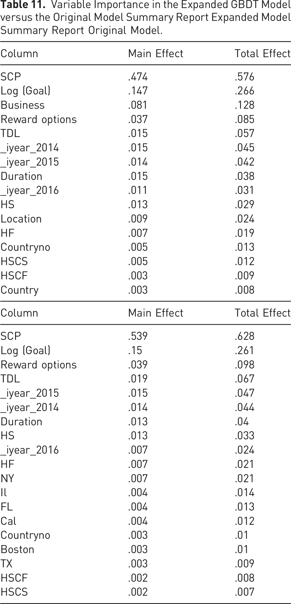
Variable Importance in the Expanded GBDT Model versus the Original Model Summary Report Expanded Model Summary Report Original Model.

Column	Main Effect	Total Effect
SCP	.474	.576
Log (Goal)	.147	.266
Business	.081	.128
Reward options	.037	.085
TDL	.015	.057
_iyear_2014	.015	.045
_iyear_2015	.014	.042
Duration	.015	.038
_iyear_2016	.011	.031
HS	.013	.029
Location	.009	.024
HF	.007	.019
Countryno	.005	.013
HSCS	.005	.012
HSCF	.003	.009
Country	.003	.008

Column	Main Effect	Total Effect
SCP	.539	.628
Log (Goal)	.15	.261
Reward options	.039	.098
TDL	.019	.067
_iyear_2015	.015	.047
_iyear_2014	.014	.044
Duration	.013	.04
HS	.013	.033
_iyear_2016	.007	.024
HF	.007	.021
NY	.007	.021
Il	.004	.014
FL	.004	.013
Cal	.004	.012
Countryno	.003	.01
Boston	.003	.01
TX	.003	.009
HSCF	.002	.008
HSCS	.002	.007

Second, the study provides some interesting insights on the nonlinear relationships between the explanatory variables and the likelihood of success for art projects. For example, the output shows the existence of threshold and Goldilocks effects, which contradicts the constant positive or negative coefficients that the literature predicts with respect to the explanatory and control variables (e.g., Butticè et al., 2017; Colombo et al., 2015; Courtney et al., 2017; Li et al., 2022; Lin & Boh, 2021; Mollick, 2014; Shneor et al., 2021; Skirnevskiy et al., 2017; Usman et al., 2020).

Third, the model imparts some insights on the effects of non-quantitative variables (text variables in this study) on the likelihood of success.

Fourth, the database used in this study will be made available to researchers and could be utilized by them to conduct research.

6.2 Practical Implication

In addition to its contribution to academic literature, this study provides some practical implications to creators of art projects. They could choose, for example, not to label the specific project domain and just use a generic “art” label, maximizing the likelihood of success, as shown in section 5.

In addition, creators of arts projects should carefully choose the optimal goal of the campaign, the number of reward options, the duration of the campaign, and the average price of reward options (TDL). In making their decisions art projects creators need to consider the fact that their decisions today also affect their future campaigns and therefore should look at this as a multiperiod game rather than a one-period one.

One of the results of this study is that creators must tap into their entire social capital striving to maximize the number of the campaign.

Last, in their decisions creators of art projects must consider the nonlinear effects of their choice on the likelihood of success (in particular, threshold and Goldilocks effects).

6.3 Limitations

This is an exploratory and pedagogical study and like all studies it suffers from some inherent limitations, some of which can be addressed in an extension to this study.

One limitation is the size of the sample. While the number of observations is large and enables robust logistic regression and tree-based machine learning modeling, it cannot be used for Deep Learning. This is a limitation that unfortunately cannot be addressed because Deep Learning models require millions of observations, a sample size that is impossible to achieve for any single platform even if we include all projects in that platform.

A second limitation, which can be addressed in an extension to this study, is that the entire sample is from one platform, Kickstarter. Kickstarter is a major non-investment platform and has been used in a myriad of studies. Nevertheless, having data from only one platform, important as it is, could potentially lead to self-selection bias due to the idiosyncrasies of the specific platform. The robustness tests that in this study potentially minimize this possibility but a better way to address this problem would be an extension to this study using data from other non-investment platforms.

A third limitation is the fact that the data relates to the period from 2013 to 2016 and, as such, things could have changed since then. Given the fact that the study is meant as a teaching tool and the data is used only to illustrate the analysis, this concern is not major. Nevertheless, this concern should be addressed in a future study.

7. Conclusion

This study aims to enhance the knowledge of crowdfunding researchers and doctoral students on the use of machine learning models. First, it provides a structured guide on the use of machine learning methods that are available for crowdfunding research and related best practices. The study also could help academics better understand what types of insights can be obtained from machine learning methods. For example, through data and information visualization. Another contribution of the study is the insights it provides on the effects of text variables on the likelihood of art projects’ success. The study also provides some interesting insights on the nonlinear relationships between the explanatory variables and the likelihood of success for art projects (e.g., threshold and Goldilocks effects).

The study also offers some practical implications to art project creators. For example, creators of arts projects could use the guidance from this study on their description of the art domain of the project, the targeted amount of the campaign, the number of reward options offered to backers, the average price of reward options, the optimal duration of the project, and how to mobilize their social capital before and during the campaign. In doing so creators need to be cognizant of the nonlinear effects of their choices on the likelihood of success, as well as the fact that their choices today affect not just current campaigns but future ones as well.

Supplemental Material

Supplemental Material for Machine Learning and Non-Investment Crowdfunding Research: A Tutorial

Supplemental Material for Machine Learning and Non-Investment Crowdfunding Research: A Primer by Ramy Elitzur in Journal of Alternative Finance

Footnotes

Declaration of Conflicting Interests

The author(s) declared no potential conflicts of interest with respect to the research, authorship, and/or publication of this article.

Funding

The author(s) received no financial support for the research, authorship, and/or publication of this article.

ORCID iD

Ramy Elitzur

Supplemental Material

Supplemental material for this article is available online.

Notes

Author Biography

Ramy Elitzur got his Ph.D. from the Stern School of Business Administration, New York University. He is a professor of accounting at the Rotman School of Management, University of Toronto. His research interests include financial reporting and auditing, venture capital, crowdfunding, entrepreneurship, machine learning, and data analytics in sports. He has published in journals such as Contemporary Accounting Research, Healthcare Management Science (part of Springer Nature journals), Journal of Business Venturing, Entreprenurship Theory and Practice, and the Journal of Business Venturing Insights.

References

Ariza-Garzón

M. -J.

Camacho-Miñano

M. -D. -M.

Segovia-Vargas

M. -J.

Arroyo

(2021). Risk-return modelling in the p2p lending market: Trends, gaps, recommendations and future directions. Electronic Commerce Research and Applications, 49(September-October), 101079.

Liu

Usman

(2017). The influence of online information on investing decisions of reward-based crowdfunding. Journal of Business Research, 71 (February), 10-18. Journal of Business Research, 71(February), 10–18. https://doi.org/10.1016/j.jbusres.2016.10.001.

Butticè

Colombo

M. G.

Wright

(2017). Serial crowdfunding, social capital, and project success. Entrepreneurship Theory and Practice, 41(2), 183–207. https://doi.org/10.1111/etap.12271

Chang

A.-H.

Yang

L.-K.

Tsaih

R.-H.

Lin

S.-K.

(2022). Machine learning and artificial neural networks to construct P2P lending credit-scoring model: A case using lending club data. Quantitative Finance and Economics, 6(2), 303–325. https://doi.org/10.3934/QFE.2022013

Chun-Yueh

(2019). Detecting the market reaction of start-ups on GISA equity crowdfunding in Taiwan by decision tree algorithm. International Journal of Performance Measurement, 9(2), 63–87.

Colombo

M. G.

Franzoni

Rossi Lamastra

(2015). Internal social capital and the attraction of early contributions in crowdfunding. Entrepreneurship Theory and Practice, 39(1), 75–100.

Courtney

Dutta

(2017). Resolving information Asymmetry: Signaling, Endorsement, and crowdfunding success. Entrepreneurship Theory and Practice, 41(2), 265–290. https://doi.org/10.1111/etap.12267

Deng

Sun

Jiang

(2022). A literature review and integrated framework for the determinants of crowdfunding success. Financial Innovation, 8(1), 41. https://doi.org/10.1186/s40854-022-00345-6

Duan

Hsieh

T. -S.

Wang

R. R.

Wang

(2020). Entrepreneurs' facial trustworthiness, gender, and crowdfunding success. Journal of Corporate Finance, 64(October), 101693. https://doi.org/10.1016/j.jcorpfin.2020.101693

10.

Elitzur

Muttath

Soberman

(2023a). Rotman School of Management, The University of Toronto. Working paper. Crowdfunding and too much choice: A recipe for disappointment.

11.

Elitzur

Katz

Muttath

Soberman

(2023b). Machine learning methods and the analysis of threshold and Goldilocks effects in reward-based crowdfunding. Rotman School of Management, The University of Toronto. Working paper.

12.

Elitzur

Krass

Zimlichman

(2023c). Machine learning for optimal test admission in the presence of resource constraints. Health Care Management Science, 26, 279–300. https://doi.org/10.1007/s10729-022-09624-1

13.

Elitzur

Solodoha

(2021). Does gender matter? Evidence from crowdfunding. Journal of Business Venturing Insights, 16, 1–12.

14.

Flach

P.A.

Hernandez-Orallo

Ferry

(2011). A coherent interpretation of AUC as a measure of aggregated classification performance. In Proceedings of the 28th International Conference on machine learning (ICML-11), pp. 657–664. Available on: https://icml.cc/2011/papers/385_icmlpaper.pdf

15.

Gourville

Soman

(2005). Overchoice and Assortment type: When and why Variety backfires. Marketing Science, 24(3), 382–395.

16.

Iyengar

S. S.

Lepper

M.R.

(2000). When choice is demotivating: Can one desire too much of a good thing? Journal of Personality and Social Psychology, 79(6), 995–1006.

17.

Jagtiani

Lemieux

(2019). The roles of alternative data and machine learning in fintech lending: Evidence from the LendingClub consumer platform. Financial Management, 48(4), 1009–1029. https://doi.org/10.1111/fima.12295

18.

Josefy

Dean

T. J.

Albert

L. S.

Fitza

M. A.

(2017). The role of community in crowdfunding success: Evidence on cultural Attributes in funding campaigns to “save the local Theater”. Entrepreneurship Theory and Practice, 41(2), 161–182.

19.

Jutasompakorn

Perdana

Balachandran

(2023). Enhancing decision making with machine learning: The case of aurora crowdlending platform. Journal of Information Technology Teaching Cases, 13(1), 58–66. https://doi.org/10.1177/20438869211060847

20.

Kaartemo

(2017). The elements of a successful crowdfunding campaign: A systematic literature review of crowdfunding performance. International Review of Entrepreneurship, 15(3), 291–318.

21.

Kim

Wattenberg

Gilmer

Cai

Wexler

Viegas

Sayres

(2018). The influence of online information on investing decisions of reward-based crowdfunding. Journal of Business Research, 71(February), 10–18. https://doi.org/10.1016/j.jbusres.2016.10.001

22.

Kim

J.-Y.

Cho

S.-B.

(2019). Towards repayment prediction in peer-to-peer social lending using deep learning. Mathematics, 7(11).

23.

Kriebel

Stitz

(2021). Credit default prediction from user-generated text in peer-to-peer lending using deep learning. European Journal of Operational Research, 302(1), 309–323. https://doi.org/10.1016/j.ejor.2021.12.024

24.

Kuppuswamy

Bayus

(2017). Does my contribution to your crowdfunding project matter? Journal of Business Venturing, 32(1), 72–89.

25.

Wang

Pan

Gao

(2022). Signaling effect in social network and charity crowdfunding: Empirical analysis of charity crowdfunding of Sina MicroBlog in China. Frontiers in Psychology, 13, 944043. https://doi.org/10.3389/fpsyg.2022.944043

26.

Liang

Frederick

D.A.

Lledo

E.L.

Rosenfield

Berardi

Linstead

Uri Maoz

(2022). Examining the utility of nonlinear machine learning approaches versus linear regression for predicting body image outcomes: The U.S. Body Project I. Body Image, 41(June), 32–45. https://doi.org/10.1016/j.bodyim.2022.01.013

27.

Liao

Zhou

Yuan

Xiong

(2018). Large-scale short-term urban taxi demand forecasting using deep learning, 2018 23rd Asia and South Pacific Design Automation Conference. ASP-DAC, pp. 428–433.

28.

Lin

Boh

W. F.

(2021). Informational cues or content? Examining project funding decisions by crowdfunders. Information & Management, 58(7), 103499. https://doi.org/10.1016/j.im.2021.103499

29.

Litjens

Sánchez

Timofeeva

(2016). Deep learning as a tool for increased accuracy and efficiency of histopathological diagnosis. Scientific Reports, 6, 26286. https://doi.org/10.1038/srep26286

30.

Sha

Wang

Yang

Niu

(2018). Study on a prediction of P2P network loan default based on the machine learning LightGBM and XGboost algorithms according to different high dimensional data cleaning. Electronic Commerce Research and Applications, 31(September-October), 24–39. https://doi.org/10.1016/j.elerap.2018.08.002

31.

MAQC Consortium . (2010). The MicroArray Quality Control (MAQC)-II study of common practices for the development and validation of microarray-based predictive models. Nature Biotechnology, 28, 827–838. https://doi.org/10.1038/nbt.1665.

32.

Mollick

E. R.

(2014). The dynamics of crowdfunding: An exploratory study. Journal of Business Venturing, 29(1), 1–16.

33.

Moscovich

Rosset

(2022). On the cross-validation bias due to unsupervised preprocessing. Journal of the Royal Statistical Society - Series B: Statistical Methodology, 84(4), 1474–1502. arXiv:1901.08974. https://doi.org/10.1111/rssb.12537

34.

Najafabadi

M. M.

Villanustre

Khoshgoftaar

T. M.

(2015). Deep learning applications and challenges in big data analytics. Journal of Big Data, 2, 1. https://doi.org/10.1186/s40537-014-0007-7

35.

Niu

Ren

(2019). Credit scoring using machine learning by combing social network information: Evidence from peer-to-peer lending. Information, 10(12).

36.

Oduro

M. S.

Huang

(2022). Predicting the entrepreneurial success of crowdfunding campaigns using model-based machine learning methods. International Journal of Crowd Science, 6(1), 7–16. https://doi.org/10.26599/IJCS.2022.9100003

37.

Peng

Zhou

Niu

Feng

(2021). Predicting fundraising performance in medical crowdfunding campaigns using machine learning. Electronics, 10(2). https://doi.org/10.3390/electronics10020143

38.

Rao

Fung

Glenn.

(2008). On the Dangers of Cross-Validation. An Experimental Evaluation. 588-596. https://doi.org/10.1137/1.9781611972788.54

39.

Rasekhschaffe

K.C.

Jones

R.C.

(2019). Machine learning for stock selection. Financial Analysts Journal, 75(3), 70–88. https://doi.org/10.1080/0015198X.2019.1596678

40.

Scheibehenne

Greifeneder

Todd

P. M.

(2010). Can there ever be too many options? A meta-Analytic review of choice overload. Journal of Consumer Research, 37(3), 409–425. https://doi.org/10.1086/651235

41.

Shalev-Shwartz

Ben-David

(2014). Understanding machine learning: From theory to algorithms. Cambridge University Press.

42.

Shneor

Liang

Flåten

B.T.

(2020). Introduction: From fundamentals to Advances in crowdfunding research and practice. In Advances in crowdfunding. Palgrave Macmillan.

43.

Shneor

Mrzygłód

Adamska-Mieruszewska

Fornalska-Skurczyńska

(2021). The role of social trust in reward crowdfunding campaigns’ design and success. Electronic Markets, 32, 1103–1118. https://doi.org/10.1007/s12525-021-00456-5

44.

Shneor

Vik

A. A.

(2020). Crowdfunding success: A systematic literature review 2010-2017. Baltic Journal of Management, 15(2), 149–182. https://doi.org/10.1108/BJM-04-2019-0148

45.

Skirnevskiy

Bendig

Brettel

(2017). The Influence of Internal Social Capital on Serial Creators’ Success in Crowdfunding. Entrepreneurship Theory and Practice, 41(2), 209–236. https://doi.org/10.1111/etap.12272.

46.

Statista . (2022). Volume of funds raised through crowdfunding worldwide in 2020, by model category. Available at: https://www.statista.com/statistics/946668/global-crowdfunding-volume-worldwide-bytype/#:∼:text=In_2020%2C_the_volume_of,through_equity%2Dbased_crowdfunding_globally

47.

Steigenberger

Wilhelm

(2018). Extending signaling theory to rhetorical signals: Evidence from crowdfunding. Organization Science, 29(3), 529–546. https://doi.org/10.1287/orsc.2017.1195

48.

Usman

S. M.

Bukhari

F. A.

You

Badulescu

Gavrilut

(2020). The effect and impact of signals on investing decisions in reward-based crowdfunding: A comparative study of China and the United Kingdom. Journal of Risk and Financial Management, 13(12). https://doi.org/10.3390/jrfm13120325

49.

Wang

Y. J.

Goh

(2021). Signaling persuasion in crowdfunding entrepreneurial narratives: The subjectivity vs objectivity debate. Computers in Human Behavior, 114(January), 106576. https://doi.org/10.1016/j.chb.2020.106576

50.

Wang

Y. J.

Goh

(2022). Linguistic information distortion on investment decision-making in the crowdfunding market. Management Decision, 60(3), 648–672. https://doi.org/10.1108/MD-09-2020-1203

51.

Woods

Huang

(2020). Predicting the success of entrepreneurial campaigns in crowdfunding: A spatio-temporal approach. Journal of Innovation and Entrepreneurship, 9(13). https://doi.org/10.1186/s13731-020-00122-8

52.

Xie

(2021). Loan default prediction of Chinese P2P market: A machine learning methodology. Scientific Reports, 11(1), 18759. https://doi.org/10.1038/s41598-021-98361-6

53.

Zhong

(2022). Success prediction of crowdfunding campaigns with project network: A machine learning approach. Journal of Electronic Commerce Research, 23(2), 99–114.

54.

Zhou

Wang

Ding

Xia

(2019). Default prediction in P2P lending from high-dimensional data based on machine learning. Physica A: Statistical Mechanics and Its Applications, 534(November), 122370. https://doi.org/10.1016/j.physa.2019.122370

Supplementary Material

Please find the following supplemental material available below.

For Open Access articles published under a Creative Commons License, all supplemental material carries the same license as the article it is associated with.

For non-Open Access articles published, all supplemental material carries a non-exclusive license, and permission requests for re-use of supplemental material or any part of supplemental material shall be sent directly to the copyright owner as specified in the copyright notice associated with the article.

0.00 MB

0.35 MB