Sage Journals: Discover world-class research

Abstract

Background: Models of collective decision-making typically assume that individuals sample information independently and decide instantaneously. In most natural and sociological settings, however, decisions occur over some timescale in which group members gather information—often from multiple sources. Information sources may persist for varying lengths of time or be viewed concurrently and identically by multiple group members. These tendencies introduce spatio-temporal correlations in gathered information with poorly understood consequences.

Research Design: Here, we develop a collective decision-making model in which individuals’ access and switch between two conflicting cues that differ in their spatio-temporal properties.

Results: Our model reveals that spatially and temporally correlated cues can profoundly affect collective decisions. Specifically, we observe that spatially correlated cues are dominant when individuals rarely switch between sources of information. Temporally correlated cues, on the other hand, have the strongest impact when individuals frequently switch between information sources. We also discuss how much the usage of independent information must be increased to counter the impact of correlation.

Conclusions: The present model represents a first step toward more accurately capturing the complex mechanisms underlying collective decision-making in natural systems and reveals multiple ways in which the properties of environmental cues can impact collective behavior.

Keywords

Collective decision-making spatio-temporal correlations wisdom of crowds drift-diffusion collective intelligence

Significance Statement

Collective decision-making describes interrelated processes by which individuals gather information from the environment and jointly reach a conclusion. It is ubiquitous across social species, from slime molds and fish schools to flocks of birds, and human societies.

Information gathered from the environment often exhibits some degree of structure in space or time—generating correlations between cues aggregated within or across individuals. Here, we extend common theoretical models of collective decision-making to examine how this structure and sampling strategies impact the accuracy of collective decisions.

In particular, we model information sources (or cues) which exhibit temporal correlations (provide the same information over multiple time steps) or spatial correlations (provide the same information to multiple individuals) and compare different sampling strategies where individuals rarely or frequently switch between information sources.

We find that cues which exhibit temporal correlation impact the collective decision most strongly when individuals frequently switch between information sources, whereas spatially correlated cues have the strongest impact when individuals mostly attend to a single cue.

Our work highlights some of the complexities which arise in more realistic decision environments and could potentially be applied to the study of collective animal behavior or the decision behavior of humans in online environments where we expect multiple and possibly correlated information sources to be the norm rather than the exception.

Introduction

Collective decision-making is ubiquitous across social species: from slime mold colonies to fish schools to human societies, individual decisions are not made in isolation but influence and are influenced by the opinions and decisions of others.

In many cases, animal groups reach a consensus when making decisions, often to maintain group cohesion and retain the benefits of group-living (Krause et al., 2002; Sumpter, 2010). A large and growing body of research has demonstrated empirically that accuracy can be improved when decisions are made collectively, for many social species and decision contexts. For example, larger fish schools are better able to avoid potential predators (Ward et al., 2008, 2011) or migrate more accurately (Berdahl et al., 2016), ant colonies are better able to identify the superior of two potential nest sites of similar quality (Sasaki and Pratt 2011; Sasaki et al., 2013), and human groups can make better decisions across a range of estimation tasks (Galton, 1907; King et al., 2012; Wolf et al., 2013), particularly in the context of medical diagnoses (Kurvers et al., 2015, 2016; Wolf et al., 2015).

However, the theoretical models that inform predictions about the behavior of organisms, and the outcome of collective decision-making processes, often remain simplistic compared to the complexity and variety of the ecological contexts in which actual decisions are made (De Condorcet, 1785; King and Cowlishaw, 2007).

Previous work has often focused on one-shot decision processes, whereas in natural settings the acquisition of information occurs across some nonzero temporal scale, ranging from millisecond responses when evading potential predators (Sosna et al., 2019) to long-timescale processes such as migration (Berdahl et al., 2018). Additionally, sources of information can dissipate at some time scale, limiting how quickly individuals can acquire information. While temporal integration of information has been studied previously, often through the use of drift-diffusion models (e.g., Bitzer et al., 2014; Tump et al., 2020; Tajima et al., 2016), these models typically assume a single information source providing independent information to all individuals in the group.

Naturally occurring information cues, by contrast, may be highly correlated in space, such as a loud noise that all of the individuals in a group can hear, or correlated in time, such as an odor plume that persists for some amount of time (Torney et al., 2009). Still other cues may be correlated in both space and time, such as the air temperature across a particular day.

Previous work has studied the impact of correlated information in one-shot decision scenarios. It has been shown that when there is a mixture of both independent information (some individuals in the group observe private information from the environment) and spatially correlated information (some individuals all observe the same information), the correlated information can have an outsized influence on the resulting collective decision (Kao and Couzin, 2014). In particular, spatial correlation can break the “wisdom of crowds” effect (higher collective accuracy with increasing group size) and lead to accuracy being maximized at relatively small group sizes. Similar effects can be observed when correlations are produced via social influence within the group itself, rather than being a property of external cues (Mann, 2021; Vicente-Page et al., 2018). Some recent studies have demonstrated ways in which groups might overcome the impact of spatially correlated information on collective decision-making, including utilizing stalemates (Winklmayr et al., 2020) or creating internal structure within the group (Kao and Couzin, 2019).

These previous studies have mostly focused on correlations in space, since in such models multiple individuals in the group, located at different positions in space, perceive the same information. Correlations in time, on the other hand, have received much less attention but are likely to be just as relevant in natural environments. Temporal correlations of information (i.e., the temporal persistence of a piece of information) on their own, or in combination with spatial correlations, may therefore impact the optimal strategy that individuals in groups should use to acquire information from the environment and make collective decisions.

In the following, we introduce a model that aims to explore some of these complexities by moving the collective decision process to the temporal domain and measuring the impact of competing information sources while explicitly considering spatio-temporal correlations in these sources. The model presented here can be considered a discrete time version of a drift-diffusion process and extends previous models of collective decision-making under spatially correlated information (such as Kao et al., 2014; Winklmayr et al., 2020) into the time domain. After a description of the model, we will study the role of cue bias in collective decisions in the presence of two uncorrelated information sources. We will then examine the impact of spatio-temporal correlations in the information sources on the collective decision and discuss measures that human or non-human animal groups could undertake in order to counter correlated information.

Methods

Model

We assume a group of N agents with opinion states ${o_{j} (t)}_{j = 1}^{N}$ . The opinion states are initialized at o_j (t₀) = 0 and at each time increment dt they are updated by increments/decrements of dx = (±1)dt as the agents perceive information from the environment. We will refer to the interval size dt as the step size of the decision dynamics. When an agent’s opinion reaches one of the symmetric decision thresholds ±θ, we consider that agent to have made a decision, which remains fixed for the rest of the simulation (i.e., the thresholds are absorbing boundaries). This process of individual integration of information is illustrated in Figure 1.

Figure 1.

Examples of cues providing uncorrelated (a), spatially (b), and temporally correlated (c) information. Top row: Each square represents one bit of information received by agent i at time t. Black squares represent a cue value of −1, white squares represent a cue value of 1. Bottom row: Evolution of the decision states of N = 5 agents attending to a cue with reliability r = 0.7.

Once all agents have reached one of the two absorbing boundaries, the collective decision is computed through simple majority rule across all individual decisions. The individuals do not interact with each other during the accumulation of information (unlike, say, Tump et al., 2020). We set θ = 1 throughout the following analysis and typically use dt = 0.1, although we discuss the effect of other values of dt (see Figure 2 (a) and (b)). Note that if dt ≥θ, this model simplifies to a one-shot decision process, identical to Kao and Couzin (2014).

Figure 2.

An overview of model properties: (a) Probability of a single individual deciding in favor of cue A’s preferred option as a function of cue reliability. Blue dashed lines represent results from simulations using dt = 0.1 and different lengths of temporal cue correlation s. Grey solid lines represent analytic results for an uncorrelated cue with different step sizes dt. (b) Expected decision time for a single individual as a function of reliability for two values of the step size dt. (c) An individual’s probability of experiencing a switch away from its current cue within the expected decision time as a function of switching rate for different values of the current cue’s bias. (d) Distribution of the usage of cue A for different values of the switching rate. If not otherwise specified we used: N = 101, r_A = 0.7, r_B = 0.3, and ρ = ρ_AB = ρ_BA.

We further assume that the agents receive information from the environment via two sources (or cues): A and B. The cues produce signals which are sampled from a Bernoulli distribution with values in {−1, +1}. Each cue is characterized by a single parameter r, such that P(A = 1) = r_A and P(B = 1) = r_B. We call r the cue’s reliability, d = sign (r−1/2) the cue’s preferred direction, and b = |r−1/2| the cue’s bias. For example, if r_A = 0.6 and r_B = 0.3, then cue A has a preferred direction of 1 and a bias of 0.1, while cue B has a preferred direction of −1 and a bias of 0.2.

Reaching a boundary

When an agent strictly attends to only one of the cues, the probability of that agent reaching the upper boundary can be calculated as follows:

\hat{r} = {\begin{array}{c} \frac{1}{{(\frac{1 - r}{r})}^{\frac{θ}{d t}} + 1}, & if r \neq 1 / 2 \\ 1 / 2, & if r = 1 / 2 \end{array}

(1)

where r is the reliability of the cue that is being attended to. This is the solution for the well-known gambler’s ruin problem (Feller, 1957), adapted for symmetric absorbing boundaries. The expected time until either boundary is reached is given by

E (T) = {\begin{array}{c} \frac{θ}{d t (1 - 2 r)} [1 - 2 \frac{1}{1 + {(\frac{1 - r}{r})}^{\frac{θ}{d t}}}], & if r \neq 1 / 2 \\ {(\frac{θ}{d t})}^{2}, & if r = 1 / 2 . \end{array}

(2)

From equations (1) and (2) it is clear that for fixed step-size dt and threshold θ, both the probability to reach a boundary and the time until the boundary is reached are determined solely by the reliability r. See Figure 2(a) and (b) for illustrations of equations (1) and (2).

Correlations

The samples produced by cues A and B may be uncorrelated, correlated in either space or time, or correlated in both space and time (Figure 1). If a cue produces (temporally or spatially) correlated signals, we will sometimes speak of a “(temporally or spatially) correlated cue.” When we speak of an “uncorrelated cue,” we mean that samples observed by different agents at time t or by the same agent at times t₁ and t₂ are independent and identically distributed (i.i.d.). A cue that is correlated in space will produce i.i.d. samples in time but display identical information to all agents at any given time t. A cue that is correlated in time displays the same information to a particular individual generally for longer than one time step but samples are i.i.d across individuals at any given time point t. The time between sample updates of a temporally correlated cue follows an exponential distribution with mean waiting time s, which corresponds to the correlation time of the cue. If the correlation time is long enough, such that an individual’s decision is based only on the integration of single persistent cue value, we again effectively recover a one-shot decision process. We can further combine the definitions of spatial and temporal correlation to produce cues that are simultaneously correlated in both space and time. Examples of agents attending to uncorrelated, spatially correlated, and temporally correlated cues are illustrated in Figure 1.

Attending to cues

At any given time t, any individual may attend to only one cue (cue A or cue B) and update its opinion according to the sample currently displayed by that cue. For example, if at time t an agent i attends to cue A and that cue displays a 1 (−1) to the agent, then the agent updates its opinion as o_i(t) = o_i (t−1) ± dt.

However, individuals may switch between cues according to a dichotomous Markov process (see, e.g., Potoyan and Wolynes, 2015). The probability of a switch from cue A to cue B per time step can be expressed as p_AB = ρ_ABdt (for sufficiently small values of ρ and dt such that ρdt ≪ 1). The probability of a switch from cue B to cue A is similarly set by p_BA. The parameters ρ_AB and ρ_BA are called the switching rates. In the limit of unrestricted integration time (i.e., infinite decision thresholds), the fraction of samples that an individual receives from cue A is

p_{A} = \frac{ρ_{B A}}{ρ_{B A} + ρ_{A B}} .

(3)

The calculation for cue B is analogous. We say that agents have a preference for cue A if ρ_BA > ρ_AB. The magnitude of the rates determines the time scale of the switching process, that is, how many switches take place in a given time interval regardless of cue preference. We therefore also refer to this value as switching speed. For example, we may compare two scenarios, one in which (ρ_AB,ρ_BA) = (1,1.5) and another in which $(ρ_{A B}^{'}, ρ_{B A}^{'}) = (3, 4.5)$ . In both cases, agents will, in the limit, attend to cue A with probability p_A = 0.6, but in the second case agents will switch between cues much more frequently.

While in the limit of infinite integration time the switching behavior will be solely determined by the rates ρ_AB and ρ_BA, the absorbing boundaries present in the current description of the model will impact the integration time, and by extension, the number of switches that an individual can experience. In particular, when an individual is attending to (an uncorrelated) cue A with reliability r_A, the probability of experiencing a switch away from that cue within the expected integration time $E (T; r)$ can be calculated as follows:

P (s w i t c h_{A \to B}) = 1 - {(1 - ρ_{A B} d t)}^{\frac{E (T; r_{A})}{d t}} .

(4)

This means that if a cue is more biased, the individual will decide more quickly and is less likely to experience a switch to the other cue. If, on the other hand, a cue has low bias, the agent will take more time to decide and is, in the meantime, more likely to experience a switch to the other cue. These results are illustrated in Figure 2(c).

Measures

In order to investigate the effect of bias, switching, and correlations in the information sources on collective decision-making, we generally use cue A as a point of reference and always assume that it is uncorrelated in both space and time, while cue B is correlated in some manner (in space, time, or both). Furthermore, we set the preferred directions of the two cues to be opposing (i.e., cue A will have a preferred direction of +1, while cue B will have a preferred direction of −1). By doing this, we effectively pit the two cues against each other and measure which cue “wins” by observing the direction of the final collective decision.

Since cue A is our point of reference, we are particularly interested in the probability of the majority reaching the preferred boundary of A, that is, the upper boundary (θ = 1). We call this probability P(A), but will also refer to it as collective accuracy or simply accuracy, which captures the notion that we consider the uncorrelated cue A to provide “better” information. By this we mean that an uncorrelated source will generally provide more bits of information and groups attending to an uncorrelated source can leverage the wisdom of crowds.

In particular, we measure collective accuracy as a function of switching rates and as a function of group size, to capture both the “external” effect of competing information sources and the “internal” effect of majority voting. If the interpretation of cues is reversed (i.e., B is considered “correct”), one can simply calculate P(B) = 1−P(A).

Additionally, we also aim to quantify how much information each cue provides to the group. To this end, we count how many samples the group receives from either cue until the collective decision has been reached and refer to the fraction of samples stemming from cue A as the usage of A. While for unrestricted integration time, the fraction of samples stemming from A can be calculated using equation (3), the presence of absorbing boundaries, bias and correlations will strongly impact how much either cue is used.

For the interpretation of the usage measure, it is important to keep in mind that the distribution of samples changes as individuals switch between cues (see Figure 2(d)). At low switching rates, each individual will attend almost exclusively to either cue A or cue B. In that case the distribution of cue usage across individuals is bimodal and a usage value of, for example, 0.6 is interpreted as 60% of individuals exclusively attending to cue A. As switching rates increase, each individual will receive a mixture of samples from both cues. This is reflected in the usage distribution following a normal distribution. In that case, a usage value of 0.6 is interpreted as each individual attending to cue A for an average 60% of its integration time.

Results

In the following section we will first discuss the effects of information mixing, beginning with two uncorrelated sources. We then continue to look at the mixing of an uncorrelated cue with a temporally correlated, a spatially correlated, and finally a cue that is both temporally and spatially correlated. In all cases, we set r_A = 0.7 and r_B ∈ {0.2, 0.3, 0.4} to understand how the relative bias of the two cues affects the results. Whenever group size is not explicitly studied as a parameter, we will assume N = 101. For the below results, we assume that the individuals have no preference for either cue, which means that at t₀, individuals are equally likely to attend to either cue, and over the course of the trial, the switching rates remain equal ρ = ρ_AB = ρ_BA. Therefore, the only free parameter is the switching speed. We will, however, explicitly discuss unequal cue preferences at the end of the results section.

The main results are summarized in Figure 3, with the columns corresponding to our three measures: collective accuracy as a function of switching rate (left), usage of cue A as a function of switching rate (middle), and collective accuracy as a function of group size (right) for “low” (less than half of the group experiences a switch) and “high” (more than half of the group experiences a switch) values of the switching rate ρ. For a more detailed summary of the switching statistics, please refer to Table 1 in the appendix.

Figure 3.

Impact of temporal and spatial correlation on individual accuracy, cue usage, and collective accuracy in a scenario of two competing cues: From top to bottom we show the effects of mixing between cue A and cue B when cue A is uncorrelated and B is (a) uncorrelated, (b) temporally correlated, (c) spatially correlated, and (d) temporally and spatially correlated. The left panel shows accuracy of a group of N = 101 individuals as a function of switching speed, the middle panel shows the average fraction of samples stemming from cue A, and the right panel shows accuracy versus group size for low and high switching rates. In all cases, we use r_A = 0.7 and r_B = ∈{0.2, 0.3, 0.4} and equal switching rates ρ_AB = ρ_BA. For rows (b)–(d), the results for two uncorrelated cues are shown as reference (light colors). (a) (left) As switching speed increases, the accuracy is dominated by the more biased cue. (middle) As switching speed increases, the more biased cue is used for larger fractions of the integration time. (right) Accuracy versus group size for two different examples of switching speeds; (b) (left) as switching speed increases, collective accuracy drops to zero for all bias ratios; (middle) as switching rates increase, the usage of cue A decreases (almost) independent of bias ratio. (right) Collective accuracy goes from wisdom of crowds at low rates to madness of crowds at high rates. (c) Similar behavior as in (a) but the spatial correlation reduces the impact of bias on accuracy. (d) (left) combination of two correlation types leads to dominance of the correlated cue even at moderate switching rates, but the collective accuracy saturates at r_B. (middle) The cue usage is determined by the temporal correlation (similar to (b)). (right) The dominace of the correlated cue prevents wisdom of crowds for both high and low switching rates.

The rows of Figure 3 indicate the different correlation types of cue B: uncorrelated (a), temporally correlated (b), spatially correlated (c), and both temporally and spatially correlated (d).

Mixing of two uncorrelated cues

For two uncorrelated cues and vanishingly small switching rates, fixed fractions of agents attend to either cue. In that case, the majority decision is determined solely by the transformed reliabilities ${\hat{r}}_{A}$ , ${\hat{r}}_{B}$ and the ratio of agents attending to the two information sources.

The leftmost panel of Figure 3(a) provides an overview of the impact of switching speed for two uncorrelated cues. Since the agents have no preference for either cue, in the absence of switching the group is equally likely to decide for either option. As the switching rate increases, the group is more likely to decide in favor of the more biased cue.

The role of bias is also illustrated in the middle panel showing the usage of cue A where we find that the group received comparatively more samples from whichever cue is more biased. This is a consequence of equation (4): firstly, because individuals attending to the more biased cue are highly likely to reach the cue’s preferred boundary and secondly because individuals attending to the other, less biased, cue are likely to experience a switch in the direction of the more biased cue. In total, this leads to the group receiving more information from the biased cue and being more likely to decide in favor of that cue’s preferred direction.

Finally, the right panel of Figure 3(a) shows the effect of group size on collective accuracy for low and high values of switching speed. Since, in this case, both cues are uncorrelated, we always see the “wisdom of crowds,” that is, a monotonic increase (or decrease) in the collective accuracy as a function of group size, depending on which cue is more biased. However, how quickly accuracy increases (or decreases) depends on the switching rate.

The case of two uncorrelated cues serves as a control when comparing the effect of temporal and spatial correlations in the following sections and is indicated in lighter colors in the background of rows (b)–(d).

Mixing with a temporally correlated cue

To study the impact of temporal correlations, we first look at the most extreme scenario where cue B is perfectly correlated in time, that is, a sample drawn from cue B will show the same value throughout the entire duration of a trial.

The leftmost panel of Figure 3(b) shows the effect of switching between an uncorrelated and a (perfectly) temporally correlated cue. When no switching takes place, the collective decision is completely dominated by cue A, but as the individuals switch cues more frequently, the collective decision becomes increasingly dominated by cue B.

The behavior at low rates is explained relatively easily: individuals attending to cue A with r_A = 0.7 are highly likely to reach the upper boundary $({\hat{r}}_{A} = 0.9998)$ . Additionally, r_B > 0 implies that a nonzero fraction of individuals attending to cue B will receive a constant sample of +1 and thus deterministically reach the upper boundary. Together, this amounts to the majority of the group typically reaching the preferred boundary of cue A. This effect increases with larger group sizes, which is why we observe the wisdom of crowds at low switching rates for all three bias ratios (third panel of Figure 3(b)).

As switching rates increase, the temporally correlated information will be distributed among increasingly large fractions of the group. Those individuals attending to cue B will be driven to the boundary faster and be less likely to experience a switch to cue A, while individuals attending to A will be slower in their decision process and thus be more likely to experience a switch away from A (see Figure 2(b) and (c)). This observation is reflected in the effective cue usage as shown in the second panel of Figure 3(b), where we see that the usage of cue A decreases as switching rates increase and even falls below the most extreme levels observed in the uncorrelated examples. Again, the effect increases with larger group sizes, which is why collective accuracy decreases with group size at high switching rates for all three bias ratios (fourth panel of Figure 3(b)).

Scaling the temporal correlation

While the extreme case of perfect temporal correlation serves well to illustrate the mechanism behind the dominance of temporally correlated information, in nature informational cues might express a more moderate level of temporal correlation. We therefore next studied the effect of intermediate temporal correlations, set by the average inter-update time s of cue B.

Figure 4 shows the effect of different values of s on collective accuracy. For simplicity, we limit ourselves here to cues with equal bias (r_A = 0.7, r_B = 0.3). Compared to the case of two uncorrelated cues shown in Figure 3(a) (right panel), where no group size effect is observed at equal bias, here we find a steady increase in collective accuracy with increasing temporal correlation at low switching rates Figure 4(a)). The explanation behind the increase is the same as in the extreme case of perfect temporal correlation: the individuals reaching the lower boundary are outweighed by the combination of individuals attending to cue A and those receiving samples of +1 from cue B. The longer the correlation time of B, the closer the result resembles that of perfect temporal correlation.

Figure 4.

Impact of intermediate temporal correlation on collective accuracy: Accuracy versus group size for cues with equal bias (r_A = 0.7, r_B = 0.3) at low (ρ = ρ_AB = ρ_BA = 0.1 (a)) and high (ρ = 1 (b)) switching rates. Cue A is uncorrelated, and the temporal correlation of cue B is scaled by the inter-update time s, with s = 1 indicating no correlation and s = ∞ indicating perfect temporal correlation. (a) At low switching rates and high temporal correlation, collective accuracy increases with group size. (b) The opposite effect is observed at high switching rates and high temporal correlation. When cue B does not exhibit strong temporal correlation, the group size has little effect on collective accuracy for either switching speed.

At higher switching rates, cue B increasingly dominates as the temporal correlation increases. In Figure 4(b), we see that cue A weakly dominates when the temporal correlation is low, but the collective decision switches to cue B at greater correlations. While the mechanics remain the same, at higher switching rates the switching rate interferes with the correlation time, such that only at perfect correlation does cue B clearly dominate the collective decision.

Scaling the switching speed

Since in the case of perfect temporal correlation the switching speed exhibits such a powerful impact on collective accuracy, we continue to study the impact of intermediate values of $ρ$ in Figure 5. When both cues are uncorrelated, and exhibit equal bias, switching at either rate has little effect on collective accuracy (Figure 5(a)). However, in the extreme case of perfect temporal correlation (Figure 5(b)), we observe a transition around ρ = 0.5: lower values of ρ lead to a wisdom of crowds effect, whereas at higher values of ρ, collective accuracy is seen to decrease with group size. While the processes governing the positive and negative effects of switching have been described above, the transition at ρ = 0.5 simply stems from the fact that at this value on average more than half of the group members will experience a switch (see inset in Figure 5(a)).

Figure 5.

Impact of intermediate values of switching rate (or speed) on collective accuracy: Accuracy versus group size for cues with equal bias (r_A = 0.7, r_B = 0.3). (a) When cue B is uncorrelated (s = 1), the switching rate does not impact collective accuracy. (b) At perfect temporal correlation, we observe a transition around a switching rate of ρ = ρ_AB = ρ_BA = 0.5: lower values of ρ lead to wisdom of crowds, whereas at higher values of ρ collective accuracy is seen to decrease with group size. (Inset) Fraction of the group experiencing a switch as a function of ρ.

Mixing with a spatially correlated cue

Figure 3(c) shows the results for mixing with a spatially correlated cue, where the samples are i.i.d. in time but identical across individuals. The results appear to be similar to the case of two uncorrelated cues; however, especially at low switching rates, we find the effect of bias to be less powerful. At low switching rates, the individuals attending to cue B will all receive identical information and thus perform a cohesive random walk, such that with probability ${\hat{r}}_{B}$ the entire subgroup will reach the upper boundary (and with probability $1 - {\hat{r}}_{B}$ the lower boundary). In a sense the subgroup acts as a single individual and benefits less from group size, a phenomenon that has been studied in Kao and Couzin (2019). The role of effective group-size reduction is particularly visible at low reliabilities, which is why the result for r_B = 0.4 (blue) of Figure 3(c) is further from the uncorrelated reference case than the result for r_B = 0.2 (orange). At higher switching rates, samples from cue B will be distributed across the entire group, thus reducing the effect of spatial correlation. In the leftmost column of Figure 3(c), this is reflected in the lines approaching the results for two uncorrelated cues.

Spatial correlation does not affect the usage of a cue, which is why the middle panel in Figure 3(c) is not different from the uncorrelated case.

At low switching rates, accuracy does not increase as steeply with group size. This due to the spatially correlated cue effectively reducing group size, which implies that larger groups are necessary to achieve the same accuracy values as in the uncorrelated case.

Mixing recovers the wisdom of crowds

In one-shot decision processes, it has been shown that spatial correlation can break the wisdom of crowds—in other words, when a certain fraction of the group receives identical albeit (relatively) reliable information, collective accuracy does not increase with group size but instead peaks at intermediate group sizes (Kao and Couzin, 2014). When cues are mixed over the span of the integration period, the impact of spatial correlation can be broken, making accuracy again a smooth function of group size. In Figure 6, the parameters are chosen to match an example from Kao and Couzin (2014): cue A is uncorrelated with r_A = 0.51 $({\hat{r}}_{A} \approx 0.7)$ , while cue B is spatially correlated with r_B = 0.495 $({\hat{r}}_{B} \approx 0.45)$ . Additionally, individuals express a preference for cue A such that ρ_BA = 1.5ρ_AB. When no mixing takes place, the problem is equivalent to a one-shot decision process with the transformed reliabilities ${\hat{r}}_{A}$ and ${\hat{r}}_{B}$ , and we observe the characteristic peak at intermediate group sizes. However, when the switching rates are increased, we find that collective accuracy smoothly increases with group size.

Figure 6.

Impact of cue switching on the effects of spatial correlation. We reproduce an example from Kao and Couzin, (2014) using r_A = 0.51, $({\hat{r}}_{A} \approx 0.7)$ , r_B = 0.495, and $({\hat{r}}_{B} \approx 0.45)$ and assume cue B to be spatially correlated. Agents have a preference for cue A, such that they initially attend to A with p_A = 0.6 and also switch preferentially toward A with ρ_BA = 1.5ρ_AB. Integration without cue switching leads to the observation of maximum accuracy at intermediate group sizes (dark green line). When switching between cues is allowed, the decrease in accuracy for large groups disappears (light green line).

Both temporal and spatial correlation

When cue B is both temporally and spatially correlated, it will display the same sample over long time periods to all the agents attending to it. In the most extreme case of perfect temporal correlation, this means that the group will only receive one single bit of information from cue B.

The leftmost panel of Figure 3(d) shows that collective accuracy decreases already at moderate switching rates and quickly approaches the correlated cue’s reliability r_B.

The dominance of cue B can be explained by the temporal correlation, as confirmed by the similarity of the middle panels in Figures 3(b) and (d). However, unlike the case of pure temporal correlation, the group cannot profit from B’s variability at low switching rates and we cannot observe the wisdom of crowds in this regime (third panel of Figure 3(d)).

Conversely, at high switching rates, the lack of variability in B leads to a less extreme decline in accuracy compared to pure temporal correlation. While the rightmost panel of Figure 3(b) (pure temporal correlation) shows a “reversed wisdom of crowds,” that is, a steady decline in collective accuracy as group size increases, the same Figure 3(d) shows that in the case of both spatial and temporal correlation, the collective accuracy does not fall below r_B.

In sum, the effective decrease in group size that stems from spatial correlation counters the “positive” effects of temporal correlations. Cue B will thus completely dominate the collective decision, even at moderate switching rates, such that both the wisdom of crowds and the reverse wisdom of crowds disappear, and the accuracy of an infinitely large group simply matches the reliability r_B of cue B.

Overcoming correlation by cue switching

So far we have seen that not only bias but also correlations in space and time can determine which of two cues will drive a collective decision. In particular, we have shown that switching between cues can increase the effect of temporal correlation, or decrease the effect of spatial correlation. Instead of (or in addition to) an adaptation of the switching strategy, agents might also express asymmetric preferences for one of the cues (expressed as ρ_AB ≠ ρ_BA). Quantifying by how much the preference for the uncorrelated cue must be increased in order to counter the impact of correlation, has the added benefit of providing an implicit measure of the correlated cue’s influence on the collective decision.

Figure 7 shows an overview of collective accuracy as a function of the group’s preference for cue A expressed as $\frac{ρ_{B A}}{ρ_{A B}}$ . Columns correspond to low and high switching rates $ρ_{A B}$ , the rows correspond to different correlation types of cue B, and the colors indicate the bias of cue B, while r_A = 0.7. Keeping the cues’ preferred directions at +1 for cue A and -1 for cue B (as before), accuracy values above 1/2 indicate dominance of cue A, whereas accuracy values below 1/2 indicate dominance of cue B.

Figure 7.

Countering correlation by asymmetric cue preference: The collective accuracy of a group of N = 101 individuals as a function of preference for cue A over cue B measured as ρ_BA/ρ_AB at 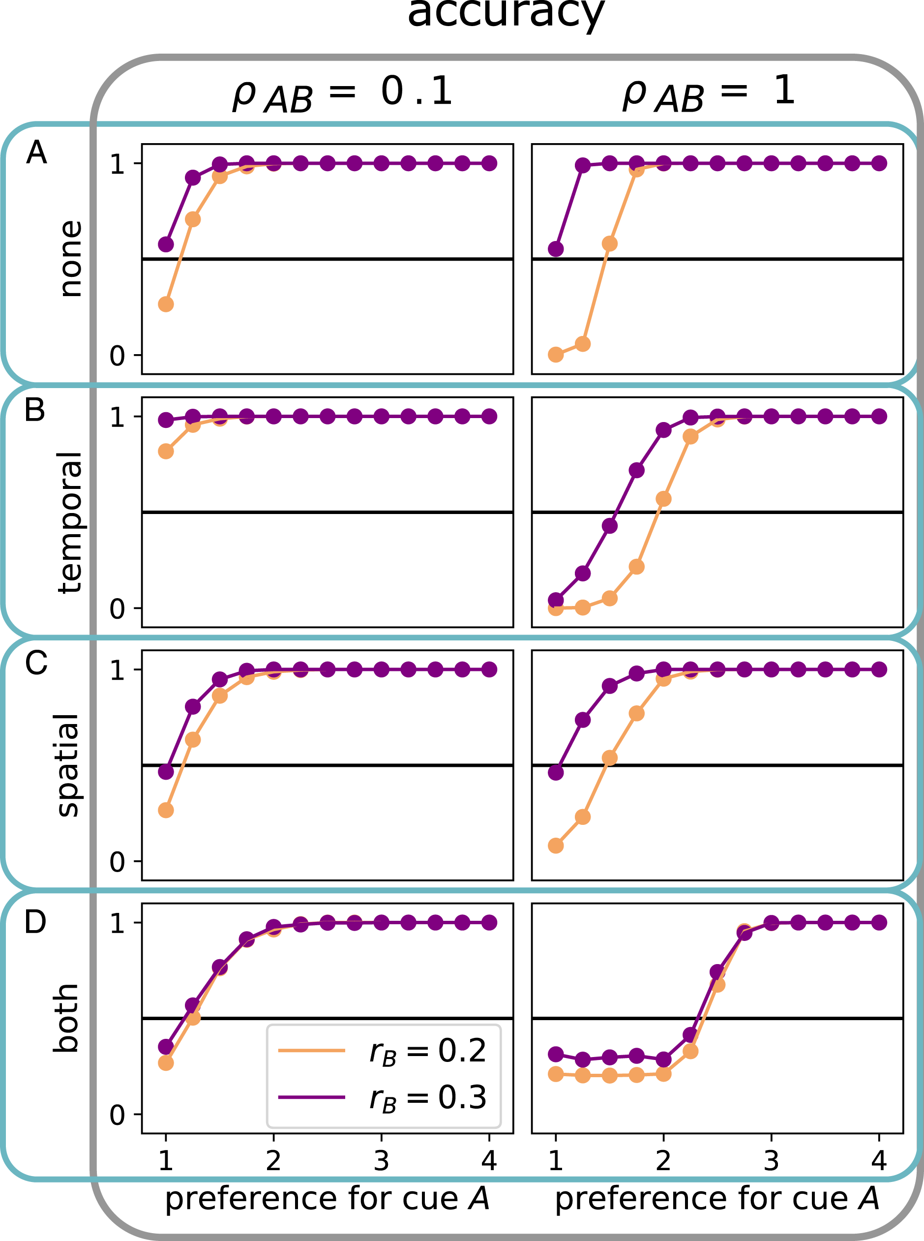$ρ_{A B} = 0.1$ (left) and ρ_AB = 1 (right). Rows correspond to different types of correlation of cue B: uncorrelated (a), temporally correlated (b), spatially correlated (c), and spatially and temporally correlated (d). In each panel, purple lines correspond to a scenario where the two cues have equal bias (r_A = 0.7, r_B = 0.3), whereas orange lines show a scenario where the correlated cue B is also more biased (r_A = 0.7, r_B = 0.2). Black horizontal lines correspond to collective accuracy of 0.5, lower values of collective accuracy indicate dominance of cue B, and higher values indicate dominance of cue A.

When biases are equal (purple curves in Figure 7), preferences are equal ( $\frac{ρ_{B A}}{ρ_{A B}} = 1$ ) and switching speed is low (left column), cue B will dominate the collective decision (i.e., collective accuracy $< 1 / 2$ ) when it is either correlated in space or both spatially and temporally correlated (left panels of rows (c) and (d) in Figure 7). When switching speed increases, cue B will dominate for all types of correlation. In particular, in the case of spatial and temporal correlation combined, the agents would need to use cue A more than twice as much to overcome the influence of cue B(right panel of Figure 7 (d)). When cue B is more biased (orange), the increase in preference for cue A necessary to compensate for cue B is greater and increases further at higher switching speeds.

Discussion

The results presented above survey the landscape of collective decision-making in the presence of multiple information sources across regimes of spatio-temporal cue correlation and relative cue strength. In particular, we studied what happens when individuals can switch their attention between two information sources and found that switching can have varying effects depending on the switching speed, the cues’ bias ratios, and whether or not either of the cues exhibits correlation.

When both cues are uncorrelated, switching can increase the impact of cue bias on the collective decision. When the information from one source exhibits temporal correlations, switching can even lead to a complete dominance over the uncorrelated information source, even if the uncorrelated source has a higher bias.

In the case of spatial correlation, the effect of switching is reversed: a spatially correlated cue exhibits its strongest impact when individuals switch between sources very little or not at all. In this case, the subgroup attending to the spatially correlated information source acts as a cohesive voting bloc that can dampen the impact of uncorrelated information. Finally, when a cue is both spatially and temporally correlated, it has a marked ability to drive collective decisions, and its influence can only be overcome by a strong preference for reliable spatio-temporal independent sources of information.

From a behavioral point of view, this means that individuals can minimize the impact of a temporally correlated information source by avoiding excessive switching. The impact of a spatially correlated source, on the other hand, can be countered by frequent switching. If, however, an information source is correlated in both space and time, changes in the switching rate will not be sufficient and a group must develop a strong preference for the uncorrelated source.

While temporal integration of a single information source has been extensively studied in the context of drift-diffusion models (e.g., Ratcliff and Smith, 2015; Wagenmakers, 2009), and there is some research on one-shot decisions in the presence of more than one cue (Kao et al., 2014; Winklmayr et al., 2020), the combination of both has, to our knowledge, not yet received much attention. Nevertheless, our model can be mapped onto these other frameworks: in the presence of a single uncorrelated cue, the present model framework can be viewed as a discrete time-step version of the well-studied drift-diffusion model (e.g., Bitzer et al., 2014; Tump et al., 2020; Tajima et al., 2016). For sufficiently large increments or small decision thresholds, where a single sample from a cue is sufficient for individuals to make a decision, the framework reduces to a single-shot decision process. For smaller increments, the model can be viewed as a single-shot decision process with transformed reliabilities ${\hat{r}}_{A}$ and ${\hat{r}}_{B}$ , as long as no switching takes place. Combined with the majority rule for collective decisions, a single-shot decision scenario either reduces to the classical “wisdom of crowds” case for fully uncorrelated information sources, or to the model proposed by Kao and Couzin (2014) in the presence of spatial correlations.

While research on collective decision-making is often focused on single-shot decisions, there is vast empirical and theoretical evidence that individual and collective decision-making is a temporal process requiring the accumulation of multiple pieces of information (Sosna et al., 2019; Tump et al., 2020). For animal groups, this accumulation may occur at different time scales, depending on the species or context. For many collective decisions, the time scale of the decision-making process may be relatively short, such as selecting a direction of motion, or choosing among available food patches. The environmental cues that individuals may utilize during these decision-making bouts may include visual, olfactory, or auditory cues. For visual cues, spatial correlations may arise when near neighbors in a group have access to similar visual information, and temporal correlations may arise if the field of view that an individual has access to is similar over some time scale. Similarly, olfactory cues are subject to currents and turbulence, and therefore the information perceived by individuals in a group will have some inherent spatial or temporal scale. Different sensory modalities may have inherently different scales of correlation. For example, auditory cues may have a longer spatial scale of correlation, as the sound travels through a group.

For some species, information accumulation and decisions may take place on a longer time scale. For example, multilevel societies of guinea baboons of vulturine guineafowl (Fischer et al., 2017; Grueter et al., 2020; Papageorgiou et al., 2019) consist of subgroups that are stable throughout the course of a day, but they may interact with other subgroups occasionally during the day. In such groups, individuals within a subgroup will have highly spatially correlated information, but information will be less correlated across subgroups (Kao and Couzin, 2019).

In natural contexts, there is no reason to assume that the spatio-temporal scale of some source of information is indicative of it being consistently well-aligned with a group’s needs and interests. Yet our results highlight multiple ways that correlations can overwhelm independent sources of information. As a consequence, decision-making rules within collectives will require taking into account not just the relative utility of two pieces of information but also their temporal and spatial characteristics.

The extent to which animals may be able to learn about correlations is not known. A theoretical model showed that it is indeed possible for individuals to collectively learn about the correlation of a cue, even when an individual cannot directly perceive the correlation (Kao et al., 2014), but this assumes that the correlation is fixed for a particular cue across multiple decision bouts. It is likely that the spatial and temporal correlation of a cue will vary across moments and days to some extent. For example, the spatial and temporal correlation of an olfactory cue will depend on the hydro- or aerodynamics of the medium on a given day. However, as we noted above, there may be, on average, consistent differences in the degree of correlation of different sensory modalities. In addition, as shown in the Supplementary Information, uncorrelated yet highly reliable signals may be difficult to distinguish from highly temporally correlated (while possibly unreliable) signals.

If it is difficult for individuals to learn about the particular levels of correlation for different environmental cues, attention switching may be a cognitively easier behavioral strategy for individuals to implement. Tuning the rate of attention switching requires an individual to know only that some temporal or spatial correlation exists in the cues, but not necessarily which cue is correlated. When attention switching is high, an individual will attend to multiple relevant cues in rapid succession, whereas when attention switching is low, an individual will fixate on a single cue for an extended period of time (a kind of “division-of-labor” approach to information gathering (Marshall et al., 2009). While little work to date has studied how social animals in a group distribute their attention across multiple environmental cues, our model suggests that the rate of attention switching may have an adaptive function in animal groups and poses specific predictions that can be tested experimentally.

One could also ask more generally about the optimality of different (collective) decision strategies in an (evolutionary) game theoretical sense. While, for example, the biased diffusion model for individual integration of evidence corresponds to optimal Bayesian updating under certain conditions (Bogacz et al., 2006), this may not be in general the case in the presence of highly correlated signals or decision-making in groups. Furthermore, the role of individual versus collective utility and the relation between optimal strategies at the individual versus collective level require further exploration. In general, for non-negligible individual-level selection, one has to expect the existence of social dilemmas where (individual-level) evolutionary stable strategies will differ from group-level optima (see, e.g., Cooney (2019), Klamser and Romanczuk (2021), Cooney et al. (2022)). While we recognize the importance of these questions, their adequate treatment goes beyond the scope of this work and should be addressed in future research.

In humans, the framing of this work has important implications for how we design and use digital communication technology (Bak-Coleman et al., 2021). Models of spatio-temporal correlations may be critical to understanding decision-making in online environments where switching between various sources is the norm rather than the exception. Disinformation campaigns are able to push a consistent narrative which may allow them to overwhelm more accurate yet evolving sources of information. We expect disinformation campaigns to be both spatially correlated (e.g., by utilizing a large army of automated bots) and temporally correlated (i.e., by broadcasting a consistent message across a long time span). As our model shows, such information sources are particularly difficult to combat. Moreover, the use of machine-learning and algorithmic recommendations have the potential to also induce spatio-temporal correlations in information, resulting in profound yet difficult to measure effects on democratic processes. The suggestion from our model that attention switching can improve collective decisions may have implications for how algorithms could be developed that increase, or decrease, switching across different information sources, in order to promote better collective societal decisions.

While our model highlights the importance of incorporating spatio-temporal features of cues, it remains an idealization. Application to a specific sociological or ecological context will require adjusting or extending features of the model. For instance, some contexts may not feature absorbing boundaries that prevent an individual from changing their mind in the future. Moreover, while the current work focuses on temporal and spatial correlations, one could also consider social interactions as a source of correlation. One possibility would be for individuals to observe others who have already decided and experience a drift toward them (Tump et al., 2020, 2021). Another extension would be to explicitly consider the relative value of options A and B for the individuals (e.g., Pais et al., 2013)—this could be achieved via cue preferences, cue bias, or increment size. A similar approach could be used to incorporate the agents’ confidence in one source over the other. Finally, one could also model the effects of more than two competing information sources.

Collectives—from animal groups to human institutions—often share information and make decisions in the face of uncertainty. Collective wisdom, or the ability to make more accurate decisions as a group, is an often-cited benefit of deciding collectively. Our results highlight how correlations across space and time can fundamentally alter collective decisions, requiring their consideration when evaluating collective intelligence in real-world contexts.

Supplemental Material

Supplemental Material - Collective decision strategies in the presence of spatio-temporal correlations

Supplemental Material for Collective decision strategies in the presence of spatio-temporal correlations by Claudia Winklmayr, Albert B Kao, Joseph B Bak-Coleman, and Pawel Romanczuk in Collective Intelligence.

Footnotes

Declaration of Conflicting Interests

The author(s) declared no potential conflicts of interest with respect to the research, authorship, and/or publication of this article.

Funding

The author(s) disclosed receipt of the following financial support for the research, authorship, and/or publication of this article: P.R acknowledges funding by the German Research Foundation via the Emmy Noether program, RO 4766/2-1, and under Germany’s Excellence Strategy EXC 2002/1 “Science of Intelligence” project 390523135. J.B-C. acknowledges funding from the John S. and James L. Knight Foundation, the UW Center for an Informed Public, the University of Washington eScience Institute, and Craig Newmark Philanthropies. A.B.K. acknowledges support from a Baird Scholarship and an Omidyar Fellowship from the Santa Fe Institute.

ORCID iDs

Claudia Winklmayr

Albert B Kao

Supplemental Material

Supplemental material for this article is available online.

References

Bak-Coleman

Alfano

Barfuss

, et al. (2021) Stewardship of global collective behavior. Proceedings of the National Academy of Sciences 118(27): e2025764118.

Berdahl

Westley

Levin

, et al. (2016) A collective navigation hypothesis for homeward migration in anadromous salmonids. Fish and Fisheries 17(2): 525–542.

Berdahl

Kao

Flack

, et al. (2018) Collective animal navigation and migratory culture: from theoretical models to empirical evidence. Philosophical Transactions of the Royal Society B: Biological Sciences 373(1746): 20170009.

Bitzer

Park

Blankenburg

, et al. (2014) Perceptual decision making: drift-diffusion model is equivalent to a Bayesian model. Frontiers in Human Neuroscience 8: 102.

Bogacz

Brown

Moehlis

, et al. (2006) The physics of optimal decision making: a formal analysis of models of performance in two-alternative forced-choice tasks. Psychological Review 113(4): 700–765.

Cooney

(2019) The replicator dynamics for multilevel selection in evolutionary games. Journal of Mathematical Biology 79(1): 101–154.

Cooney

Morris

Levin

, et al. (2022) Social dilemmas of sociality due to beneficial and costly contagion. arXiv preprint arXiv:2202.09905.

De Condorcet

(1785) Essai Sur l’Application de l’Analyse à la Probabilité Des Décisions Rendues à la Pluralité des Voix. Paris: Imprimerie Royale.

Feller

(1957) An Introduction to Probability Theory and Its Applications. New York, NY: Wiley.

10.

Fischer

Kopp

Dal Pesco

, et al. (2017) Charting the neglected west: the social system of guinea baboons. American Journal of Physical Anthropology 162: 15–31.

11.

Galton

(1907) Vox populi (the wisdom of crowds). Nature 75(7): 450–451.

12.

Grueter

Zinner

, et al. (2020) Multilevel organisation of animal sociality. Trends in Ecology & Evolution 35(9): 834–847.

13.

Kao

Couzin

(2014) Decision accuracy in complex environments is often maximized by small group sizes. Proceedings of the Royal Society B: Biological Sciences 281(1784): 20133305.

14.

Kao

Couzin

(2019) Modular structure within groups causes information loss but can improve decision accuracy. Philosophical Transactions of the Royal Society B 374(1774): 20180378.

15.

Kao

Miller

Torney

, et al. (2014) Collective learning and optimal consensus decisions in social animal groups. Plos Computational Biology 10(8): e1003762.

16.

King

Cheng

Starke

, et al. (2012) Is the true ‘wisdom of the crowd’to copy successful individuals? Biology Letters 8(2): 197–200.

17.

King

Cowlishaw

(2007) When to use social information: the advantage of large group size in individual decision making. Biology Letters 3(2): 137–139.

18.

Klamser

Romanczuk

(2021) Collective predator evasion: putting the criticality hypothesis to the test. Plos Computational Biology 17(3): e1008832.

19.

Krause

Ruxton

, et al. (2002) Living in Groups. Oxford, UK: Oxford University Press.

20.

Kurvers

Herzog

Hertwig

, et al. (2016) Boosting medical diagnostics by pooling independent judgments. Proceedings of the National Academy of Sciences 113(31): 8777–8782.

21.

Kurvers

Krause

Argenziano

, et al. (2015) Detection accuracy of collective intelligence assessments for skin cancer diagnosis. JAMA Dermatology 151(12): 1346–1353.

22.

Mann

(2021) Collective decision-making under changing social environments among agents adapted to sparse connectivity. arXiv preprint arXiv:2110.13543.

23.

Marshall

Bogacz

Dornhaus

, et al. (2009) On optimal decision-making in brains and social insect colonies. Journal of the Royal Society Interface 6(40): 1065–1074.

24.

Pais

Hogan

Schlegel

, et al. (2013) A mechanism for value-sensitive decision-making. PloS One 8(9): e73216.

25.

Papageorgiou

Christensen

Gall

, et al. (2019) The multilevel society of a small-brained bird. Current Biology 29(21): R1120–R1121.

26.

Potoyan

Wolynes

(2015) Dichotomous noise models of gene switches. The Journal of Chemical Physics 143(19): 11B612_1.

27.

Ratcliff

Smith

(2015) Modeling simple decisions and applications using a diffusion model. In: Busemeyer

Wang

Townsend

, et al. (eds), The Oxford Handbook of Computational and Mathematical Psychology. Oxford, UK: Oxford University Press, 35–62.

28.

Sasaki

Granovskiy

Mann

, et al. (2013) Ant colonies outperform individuals when a sensory discrimination task is difficult but not when it is easy. Proceedings of the National Academy of Sciences 110(34): 13769–13773.

29.

Sasaki

Pratt

(2011) Emergence of group rationality from irrational individuals. BMC Ecology 22(2): 276–281.

30.

Sosna

Twomey

Bak-Coleman

, et al. (2019) Individual and collective encoding of risk in animal groups. Proceedings of the National Academy of Sciences 116(41): 20556–20561.

31.

Sumpter

(2010) Collective Animal Behavior. Princeton, NJ: Princeton University Press.

32.

Tajima

Drugowitsch

Pouget

(2016) Optimal policy for value-based decision-making. Nature Communications 7(1): 1–12.

33.

Torney

Neufeld

Couzin

(2009) Context-dependent interaction leads to emergent search behavior in social aggregates. Proceedings of the National Academy of Sciences 106(52): 22055–22060.

34.

Tump

Pleskac

Kurvers

(2020) Wise or mad crowds? the cognitive mechanisms underlying information cascades. Science Advances 6(29): eabb0266.

35.

Tump

Wolf

Romanczuk

, et al. (2021) Avoiding costly mistakes in groups: The evolution of error management in collective decision making. PsyArXiv. DOI: 10.31234/osf.io/r4kd7.

36.

Vicente-Page

Pérez-Escudero

de Polavieja

(2018) Dynamic choices are most accurate in small groups. Theoretical Ecology 11(1): 71–81.

37.

Wagenmakers

(2009) Methodological and empirical developments for the ratcliff diffusion model of response times and accuracy. European Journal of Cognitive Psychology 21(5): 641–671.

38.

Ward

Herbert-Read

Sumpter

, et al. (2011) Fast and accurate decisions through collective vigilance in fish shoals. Proceedings of the National Academy of Sciences 108(6): 2312–2315.

39.

Ward

Sumpter

Couzin

, et al. (2008) Quorum decision-making facilitates information transfer in fish shoals. Proceedings of the National Academy of Sciences 105(19): 6948–6953.

40.

Winklmayr

Kao

Bak-Coleman

, et al. (2020) The wisdom of stalemates: consensus and clustering as filtering mechanisms for improving collective accuracy. Proceedings of the Royal Society B 287(1938): 20201802.

41.

Wolf

Krause

Carney

, et al. (2015) Collective intelligence meets medical decision-making: the collective outperforms the best radiologist. PloS One 10(8): e0134269.

42.

Wolf

Kurvers

Ward

, et al. (2013) Accurate decisions in an uncertain world: collective cognition increases true positives while decreasing false positives. Proceedings of the Royal Society B: Biological Sciences 280(1756): 20122777.

Supplementary Material

Please find the following supplemental material available below.

For Open Access articles published under a Creative Commons License, all supplemental material carries the same license as the article it is associated with.

For non-Open Access articles published, all supplemental material carries a non-exclusive license, and permission requests for re-use of supplemental material or any part of supplemental material shall be sent directly to the copyright owner as specified in the copyright notice associated with the article.

0.00 MB

0.23 MB