Sage Journals: Discover world-class research

Abstract

Time series tools are part and parcel of modern day research. Their usage in the biomedical field; specifically, in neuroscience, has not been previously quantified. A quantification of trends can tell about lacunae in the current uses and point towards future uses. We evaluated the principles and applications of few classical time series tools, such as Principal Component Analysis, Neural Networks, common Auto-regression Models, Markov Models, Hidden Markov Models, Fourier Analysis, Spectral Analysis, in addition to diverse work, generically lumped under time series category. We quantified the usage from two perspectives, one, information technology professionals’, other, researchers utilizing these tools for biomedical and neuroscience research. For understanding trends from the information technology perspective, we evaluated two of the largest open source question and answer databases of Stack Overflow and Cross Validated. We quantified the trends in their application in the biomedical domain, and specifically neuroscience, by searching literature and application usage on PubMed. While the use of all the time series tools continues to gain popularity in general biomedical and life science research, and also neuroscience, and so have been the total number of questions asked on Stack overflow and Cross Validated, the total views to questions on these are on a decrease in recent years, indicating well established texts, algorithms, and libraries, resulting in engineers not looking for what used to be common questions a few years back. The use of these tools in neuroscience clearly leaves room for improvement.

Keywords

principal component analysis time series artificial neural network auto regression markov model hidden markov model fourier analysis stack overflow cross validated pubMed neuroscience spectral analysis empirical analysis

Introduction

A time series comprises data recorded in a temporal manner. Generally, it is a succession recorded at uniformly distant positions. Time series forecasting is a technique to predict values based on historically recorded values. Conversely, time series analysis aims to obtain significant statistics from time series, which can be applied to real-world, continuous, or discrete numeric data. Time series can be used in any domain involving temporal measurements; thus, it finds application in a wide range of domains, such as statistics, weather forecasting, electroencephalography, electrocardiogram, etc.¹ In addition, time series data, which comprises numerical fields ordered chronologically, is always considered a whole instead of individual fields. Therefore, it requires specialized tools, known as time series tools, for the analysis.

In the last decade, the developments in Neuroscience involve a considerable increase in the size, dimensionality, and complexity of neural data.^2,3 Much of these data are multi-dimensional, complex, and often cross multiple levels of organizations, such as neurons, circuits, systems, whole brain, etc.^4,5 Deriving statistical inferences from these data heavily rely on the advances in time series tools. It is well established that no single tool can be chosen as the best for analysis in different situations.^6-8 Hence, an evaluation of all major approaches is needed to determine the existing state-of-the-art in the area. Here, we quantify the usage of time series tools from engineering, biomedical, and neuroscience point of view, so that researchers can understand the trends and wisely use the right tool for their applications.

Time series tools can be categorized in varied ways. Some of the possible categorizations are time and frequency domain, univariate and multivariate, parametric and non-parametric. For the initial study, we have selected 7 classical tools and categorized them based on time and frequency domain. These tools are Principal Component Analysis (PCA), Neural Networks, ARMA-ARIMA (ie, Autoregressive moving average, Autoregressive integrated moving average) Models, Markov models, Fourier analysis, and Spectral analysis.

We undertake a twofold data-driven stance to quantify the state-of-the-art practices and trends related to the utilization of these tools. Firstly, to examine the recent developments from the perspective of IT-practitioners, programmers, and statisticians, we mine knowledge from community-driven popular Q&A websites: Stack Overflow and Cross Validated. The number of questions posted, number of accepted answers, views gathered, and content of the discussion were analyzed for twelve years. Subsequently, we emphasize the application of these tools in the biomedical sector, along with neuroscience, by quantifying the vast indexed database of PubMed. In addition, we conduct a rigorous literature survey for each tool to delineate their usage patterns among researchers.

Methods

Selection of time series tools and literature survey

We select 7 time series tools and split them into time and frequency domain. The tools, namely ARMA-ARIMA, Markov model, and Hidden Markov model, are time domain tools, whereas Fourier and Spectral Analysis are frequency domain. In addition, PCA and Neural Networks are categorized as general time series tools due to their usage in both the time and frequency domain (Supplemental Figure S1).

Stack overflow and cross validated analysis

Stack Overflow (SO), founded in 2008, is the largest community-driven question and answer (Q & A) website for IT practitioners, professionals, and enthusiast programmers. It features questions on a multitude of concepts in computer programming and information technology, ranging from software engineering, data science, machine learning to statistics. The link of stack overflow is https://stackoverflow.com/, and additional summary information is available on Wikipedia https://en.wikipedia.org/wiki/Stack_Overflow.

Cross Validated (CV) is a specially oriented website of Stack Exchange, https://stats.stackexchange.com/ network that features questions related to statistics, machine learning, data analysis, data mining, and data visualization. Summary of Stack Exchange can be found at https://en.wikipedia.org/wiki/Stack_Exchange. At the time, this analysis was conducted (3rd June 2019), the corpus consists of more than 42K time series tools related questions with approximately 1000 views per question (Supplemental Table S1).

To identify time series related questions, tags of each question posted at SO and CV were analyzed. IT-practitioners asking questions on these websites tend to provide a set of tags that accurately describes their question. These tags provide categorization to each question posted on these websites. Time series-related tags across each tool were manually selected and reported in Supplemental Table S2. The questions with at least 1 time series-related tag were selected for the analysis.

Each time series tool is analyzed based on the following parameters:

1) The number of questions posted from Jan 2008 to June 2019: this parameter provides us metric to understand the interest gathered around each time series tool among IT-practitioners and how this interest has evolved in the last 12 years.

2) The number of questions with an accepted answer: this parameter provides us the metric of satisfaction of users asking time series-related questions, as users asking a question can accept an answer that accurately and correctly answers users’ queries. Higher accepted answers corresponding to a time series tool indicate the satisfaction of the user.

3) Viewership: this parameter provides us the metric of visibility of time series tools. Higher the visibility of a time series tool, higher is the ease of availability of the necessary resources related to it, ranging from the methodology of usage to solutions of errors and bugs. Mean views have also been plotted corresponding to every year, providing an overall picture for the analysis. Sometimes, the mean views are observed to be higher than the maximum in the boxplot because the mean (or average) is susceptible to extreme values. On the contrary, the boxplots are created after the removal of outliers for visual aid.

4) Additionally, the content of questions related to each time series tool was studied to gain insights. A corpus of questions was created by aggregating the title and description of each question across various time series tools. All the embedded HTML code, along with special characters and stop words, were removed from the corpus. Word Clouds of discussion for each time series tool were created, where the size of a word represents its frequency.

PubMed analysis

PubMed is a search engine that indexes biomedical and life sciences research. Analysis of time series related research indexed in PubMed was used to study the use of time series tools in biomedical research and specifically neuroscience. The title, abstract, and text word of relevant PubMed articles were analyzed to determine the presence of several time series tools. Assessment of the evolution of these tools within Neuroscience domain is conducted by identifying time series related research on PubMed with keywords “Neuroscience,” “Mental Health,” “Brain,” “Mental Illness,” “Neurology,” “Psychology,” “Depression,” “Anxiety,” “Neurodegeneration,” “Mania,” “Schizophrenia,” “Delusion,” “Alcohol,” “Alcoholism,” “Addiction,” “Aggression,” “Violence,” “Neurophysiology,” and lumped the results together. This approach will approximate the results for the Neuroscience domain as the underlying limitation of this approach is that it would not be able to identify some small fraction of papers, which might not have any of these keywords in them and yet belong to neuroscience. The search commands used to explore the results are illustrated in Supplemental Table S3. The research papers indexed on PubMed are accounted on and before 5 October, 2019.

Throughout the analysis of Stack-overflow, Cross-validated, and PubMed, we observed a sudden fall in 2019. it is due to the fact that data were not available for the complete year.

General tools for time series analysis

Principal component analysis

PCA is a well-established linear dimensionality reduction approach that has been extensively used by the researchers.⁹ It is used to convert potentially correlated variables to linearly uncorrelated principal components by the orthogonal transformation. In 1933, PCA was coined by an American statistician and an influential economist H. Hotelling,⁷ who was inspired by the principal axis theorem, given by Karl Pearson.⁶ Conventional statisticians used PCA as a dimensionality reduction tool; however, in recent developments, researchers have exploited latent properties of PCA to identify patterns within the data.

A considerable increase in time series data is observed across all domains, especially in business, medical, and scientific databases.¹⁰ Analyzing a large multi-dimensional time series is a well-established limitation. Among others, these limitations have hindered the way for determining patterns associated with stocks, identifying aberrations in an online monitoring system, recognizing non-obvious relationships between 2 time series, and hypothesis testing among time series.¹¹ In the past, large multi-dimension time series have created challenges on multiple fronts, such as clustering,¹² classification,^13,14 and mining of association rules.¹⁵ Recently, such time series pose challenges to scalable computing,¹⁶ data sharing, and reproducibility.¹⁷ Several methods were developed to speed up the analysis of large time series; however, research shows that dimensionality reduction has emerged as the most prominent method.¹⁰ Moreover, dimensionality reduction is crucial to the analysis of neural data, which are often large and multi-dimensional.¹⁸ It includes data (1) with cross multiple organizational levels (eg, neurons, circuits, and brain) or (2) involving various biological domains (eg, anatomical and functional connectivity, genetic patterns and disease states, etc.). Therefore, dimensionality reduction plays a crucial role in time series analysis.

Applications

PCA is used in Bi-plot graphic display of matrices, which is often used to represent any matrix of rank two, comprising a vector for each cell of the matrix. Vector for an element is selected so that the inner product of vectors corresponding to its row and column yields the element. Notably, the rank corresponds to the maximum count of linearly independent columns in the vector space. Subsequent to PCA analysis, bi-plots depict interunit lengths and clustered units. In addition, they delineate variances, correlation and allows the visual appraisal of large data matrices structures.¹⁹

PCA has also been used as a tool for estimation and analysis. For instance, it is used to estimate the origin of heavy metal pollution in sediments, which was conducted at Rybnik Reservoir, Southern Poland.²⁰ Moreover, PCA is utilized to analyze the timely variance of loading of trace components in bottom sediments.²⁰

PCA has medical applications as a method for the pattern analysis.²¹ A knee osteoarthritis research was administered on fifty subjects, who suffered from end-stage knee osteoarthritis; in addition, it comprises an age representative control group of 63 subjects. Gait data is represented as temporal waveforms depicting joint measurements throughout the gait cycle. Feature space comprising temporal waveforms of n subjects on p variables were constructed. These features include knee alignment variables and bone geometry data. The analysis focused on 3 gait waveform measures: the knee flexion angle, flexion moment, and adduction moment. The aim was to determine the biomechanical features of these gait measures related to knee osteoarthritis. Hypothesis testing was done to identify group differences, and discriminant analysis to (1) quantify overall group difference, and (2) establish a hierarchy of discriminatory ability among the gait waveform features. The authors analyzed this feature space by using PCA analysis, not only as a data reduction tool but also as a method for further differential analysis.^22,23 It was found that there exists a strong correlation between gait waveforms with respect to time. The study also proved that PCA can be used as a method of kinetic and kinematic analysis of gait waveforms.

Limitations

Underlying assumptions for the optimal working of PCA is that correlations in the data are linear. To address this limitation, Nonlinear Principal Component Analysis (NLPCA) was proposed that uses auto-associative neural networks.²⁴ It aims to create an identity map by learning a feedforward network such that input variables are recreated at the output layer. This neural net comprises lesser nodes as compared to the input or output layers; thus, it enables the production of a concise depiction of the variables.

Inferences from PubMed

PCA being a general purpose statistical technique, also has a style of reasoning. It is used as a ‘hypothesis generating’ tool, creating a statistical mechanics framework for biological systems modeling, without making any prior theoretical assumptions. For this very reason, it has been used in drug discovery and biomedical research.²⁵ For example, it was used as a truncation technique in the study of the classification of Mycobacteria using Raman spectra,²⁶ where the group compared classification accuracies after applying PCA and LDA (Linear discriminant analysis) with principal component selection methods across various centering and scaling options.

Multistage PCA (MSPCA) has been used for the study of abdominal electrocardiogram decomposition.²⁷ MSPCA aims to identify the variables that can be well estimated by a linear model. It involves 2 steps: top-down and down-top steps. The top-down step identifies an initial solution recursively, whereas the down-top step is introduced to penalize the maximum number of phases of the final solution.²⁸ To rephrase, dimensionality reduction is achieved by the eigenvectors with the most significant eigenvalues as a new orthonormal basis.²⁹ The electrical activity of the fetal heart has comparatively less energy; therefore, traditionally recommended component analysis fails to separate the 2 ECG signals: maternal and fetal ECGs. Thus, step-by-step extraction of abdominal ECG signal components, using multistage PCA is preferred. In addition, it has been used to create a simplistic aging equation that aims to predict the age by combining several biological factors of aging.³⁰ In one study, PCA revealed specific technical features that appeared to relate to skiers’ performance levels.³¹ In a recent modification to PCA, poorly dimensioned data can also be processed, while maintaining the data clustering capacity.³² Figure 1 looks at the trends of PCA use.

Figure 1.

Quantification of trends related to PCA. (a) Although the beginning is marked by limited PCA related questions, they gather substantial views. This suggests that the developers and researchers were looking for a platform to discuss PCA, and SO & CV facilitated them; however, the quality of discussions seemed to discourage the users, which can be observed from a huge decline in the viewership in 2011. The number of questions depicts a linearly increasing trend that can be attributed to the use of PCA in several studies as a dimensionality reduction tool.^9,33-35 One of the breakthroughs was the use of PCA in integrated dynamic analysis of the metro project.³⁶ The number of accepted answers resembles a bell-curve, that is, being constant in the period 2014-16, while following a slight decrease in 2018. (b) The boxplot shows that the mean number of views gained its highest value in 2010, that is, 35 000 views. Subsequently, a drastic fall is observed to approximately 5000 views in 2011, followed by a steady decrease. Moreover, 50% of the questions have less than 5000 views and the median value is close to quartile 1. (c) Among other generic PCA related terms, the discussion frequently mentions terms, such as data, variable, matrix, features, dimensions, and eigenvectors. Eigenvalues of the covariance represent the core of PCA. Eigenvectors help in determining the direction of the feature space, whereas the eigenvalues represent the magnitude. (d) We observe a gradual increase in the life sciences and biomedical related studies. Conversely, there are few studies on the intersection of neuroscience and PCA.

Neural network

The neural network is inspired by the nervous system.^37,38 Its theoretical framework is formulated by McCulloch³⁹ and Pitts,⁴⁰ a neuroscientist and a logician. The authors derive motivation from the core idea of a neuron, that is, a cell living within a cell network. Each neuron acquires input and produces the output after computation.

The fundamental building blocks of these networks are neurons.⁴¹ The neural network consists of interlinked neurons; each neuron comprises an activation function.⁴⁰ In a neural network, nodes represent neurons, whereas edges represent weighted neural interactions. Inputs are multiplied with the edge weight, then passed to the next layer as inputs. Generally, these networks comprise an input and output layer, along with some hidden layers.

Input to each node is calculated as follows,

F (x) = b + w 1 \cdot x 1 + w 2 \cdot x 2 + \dots + wn \cdot xn,

(1)

Yin = b + W • . X,

(2)

where Wi are the weights associated with each arc, Xi is the values at each node, and b is the bias, which is added to each layer.

After each node has received input, the activation function is applied, which further decides a node has to fire or not. There are many activation functions available such as Tanh, Sigmoid, and ReLU are (rectified linear unit) (see equations 3-5). Among them, sigmoid and relu are widely used in real-life applications. Then, the value obtained after applying the activation function is passed as the input to neurons of the different layers. This is performed for many iterations, and weights are updated after each iteration.

F (x) = 1 / (1 + e^{\land} - x)

(3)

Tanh (x) = 2 / (1 + e^{\land} (- 2 x)) - 1

(4)

F (x) = \max (0, x)

(5)

Applications

The neural network has been extensively studied, which has led to its application in diversified fields, such as business applications, forecasting, classification, pattern recognition, and time series prediction. In addition, the neural network is being utilized on a day-to-day basis in real-world business applications, such as making stock market prediction,⁴¹ which weighs many factors, for example, the rise and fall of stocks. The neural network can process the time series data, analyze its pattern, and predict stock prices. Apart from that, it is used for e-commerce fraud detection through credit cards,^42,43 money laundering detection, and telecommunication fraud,⁴⁴ that is, a neuro-fuzzy model for predicting business bankruptcy.

Deep learning is referred to as combining several layers of the neural network to perform feature engineering, along with extracting latent features from the data.⁴⁵ The deep learning technique is highly advantageous, as it can process more complex information with high accuracy but requires a large dataset for training (or learning). For instance, Dialog-Tech facilitates a system for call attribution and conversion.⁴⁶ They use the neural network to classify inbound calls into predetermined categories or assign lead quality scores based on the call transcription and the marketing channel or keyword that drove the call.⁴⁷ This process required a considerable amount of historical data for training.

The neural network finds application in classification domain, such as Internet traffic classification,⁴⁸ using Bayesian neural networks without using the source or destination port information. It works by extracting the features from packet streams consisting of 1 or more packet headers pattern classification.⁴⁹ Image classification in medical imaging and signal processing is undergoing cutting-edge development.⁵⁰ It involves the detection and classification of tumors and X-rays, along with diagnostic systems for cancer and heart diseases.⁵¹

Another application can be seen on LinkedIn that is a social networking site for professionals.⁴⁶ It uses the neural network along with text classifiers to (1) filter out the spam or abusive content from the user’s feed, (2) improve their recommendation system, and (3) search relevant products for members and customers. In addition to business forecasting, ANNs have been designed for forecasting tourism⁵² in the Balearic Islands (Spain) and monthly energy⁵³ demand using the time series data for the last 6 years. Most artificial intelligence has neural networks at the heart of operations.

Inferences from PubMed

The neural network has been used to detect diabetic retinopathy⁵⁴ from a local diabetic retinal screening program. The study achieved sensitivity and specificity closer to 80% on the international and domestic databases (New Zealand). In addition, it has been used in colorization, that is, conversion of grayscale image to a colored one, which is supposed to be a challenging task since it requires labeling scribbles on the target images manually, or curation of a diverse set of colored reference images.⁵⁵ An electrocardiogram beat classification system was implemented by BIRCNN, that is, Bidirectional Recurrent Neural Network (BIRNN) combined with Convolutional Neural Network (CNN). The morphological features were drawn out using CNN, followed by considering them in the context using BIRNN.⁵⁶

In a study, a neural network was implemented with an auto organizing radial basis function to enhance accuracy and parsimony. The authors used an adaptive version of the swarm optimization algorithm, popularly known as Adaptive Particle Swarm Optimization (APSO).⁵⁷ Fine-tuning of weights and avoidance of local optimal is achieved by using non-linear regression. In addition, APSO is used to optimize the scale and parameters of the neural network with a radial basis function. Therefore, it efficiently produces a concise model that yields high accuracy. Producing accurate surgical simulations is essential in the medical domain. The neural network was used to generate a lifelike and stable simulation of soft tissue deformation in real-time.⁵⁸ (Figure 2).

Figure 2.

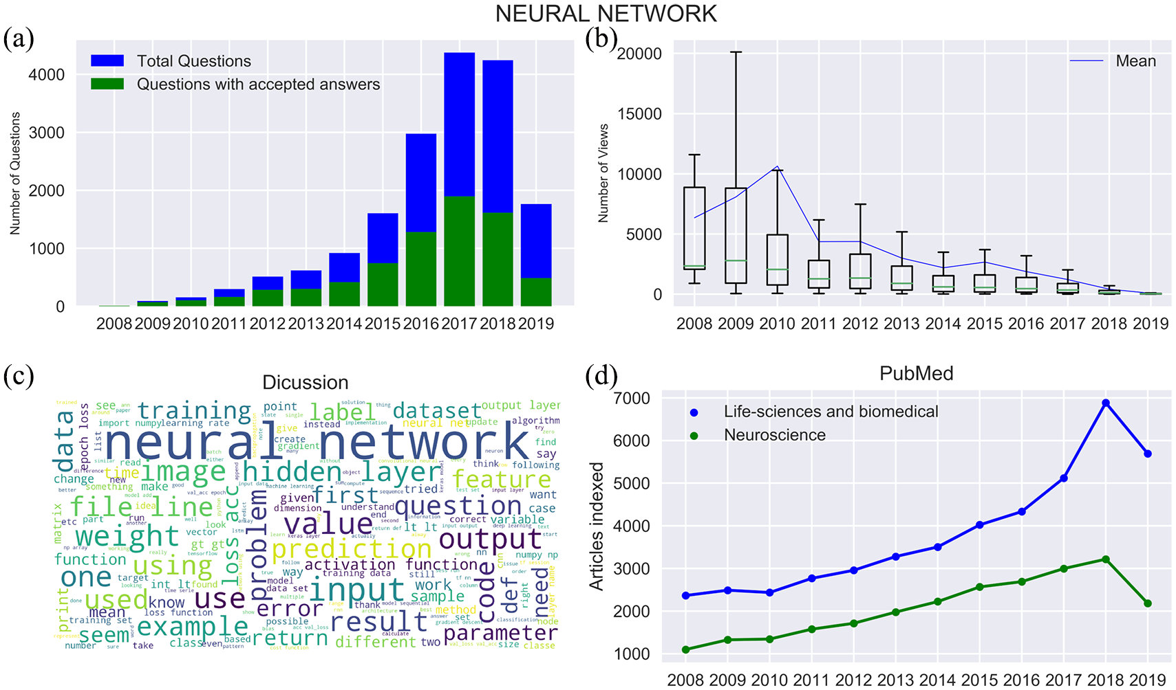
Quantification of trends related to neural networks. (a) The footprint of the neural network is visible from the beginning. The questions and accepted answers show an increasing trend. (b) A considerable amount of viewership is observed initially; however, approximately 50% of questions got less than 3K views throughout the time span. After 2009, there has been non-uniformity in the views gathered by questions as the mean views lie above the third quartile (mean value is susceptible to outliers). (c) The content of discussion frequently includes terms, such as the hidden layer, input, output, training, prediction, feature, activation function, and image. The mention of the term ‘image’ highlights the importance of CNN in the neural network domain. (d) The number of articles indexed in life sciences and biomedical resembles a polynomial growth. Approximately 7K life sciences related articles utilized the neural network in 2018, which was approximately 2200 articles in 2008. In neuroscience, the number of articles indexed has approximately increased from 1K to 3K between 2008 and 2018. The neural network is the most used time series tool in neuroscience research (also refer Figure 9).

Tools for time domain analysis

ARMA and ARIMA models

Two univariate models that represent stochastic dependence of time series data are ARMA and ARIMA models. Among others, they are useful in predictions of epidemiologic time series. They follow the “Box-Jenkins” approach.⁵⁹

ARMA model

Autoregressive (AR), when combined with the moving average (MA) model, forms the ARMA model. It was introduced by Peter Whittle in 1951⁶⁰ and has been widely used since 1970 after getting mentioned in the book by Box and Jenkins. Let us assume a continuous and equally spaced time series $z t, z t - 1, z t - 2, \dots$ with $E (z t) = 0$ . Let $a t, a t - 1, a t - 2 \dots$ be the white noise with zero mean and constant variance, where present observation can be dependent on past observations. AR Model exhibits the present observation $z t$ , that is, linearly dependent on previously recorded $z t - 1$ and white noise variable at:

zt = φ zt - 1 + at,

where ϕ is called the auto-regression parameter, as $z t$ is regressed over $z t - 1$ with order 1 as 1 observation from the past is regressed. This model is denoted by $A R (p)$ with $p$ equal to unity.

Consider a generalized AR model of order p:

z t = φ 1 z t - 1 + \cdot \cdot \cdot + φ p z t - p + a t .

(6)

MA model represents $z t$ as a linear combination of present and previous white noise:

z t = a t - θ a t - 1,

where $θ$ is a parameter. This is called the MA model of order one and is denoted by $M A (q)$ , where $q = 1$ . Consider a generalized MA model of order q:

zt = at - θ 1 at - 1 - \cdot \cdot \cdot - θ qat - q .

(7)

Thus, by combining equations 6 and 7, we obtain $A R M A (p, q)$ model (equation 8),

zt = φ 1 zt - 1 + \cdot \cdot \cdot + φ pzt - p + at - θ 1 at - 1 - \cdot \cdot \cdot - θ qat - q .

(8)

ARIMA model

Box and Jenkins⁵⁹ extended the early work of Yule and Wold^61,62 to develop the ARIMA model to include the degree of integration to which the series has been differentiated to obtain a stationary series. $A R I M A (p, q)$ is a stationary model with classical assumptions. The covariance of a stationary series depends only on the difference between 2 points with constant mean and variance.

Suppose a non-stationary time series; however, the series of its first differentiation is stationary (see equation 9), where ∇ is an ordinary differentiating operator.

wt = zt - zt - 1 = \nabla zt

(9)

Consider a series that is differentiated d times to obtain stationary status; then, the model is called integrated ARIMA model of order p, d, q, or ARIMA.

Box-Jenkins approach

ARIMA models are realized using the Box-Jenkins approach. Box-Jenkins model includes identification, estimation, and diagnostic check.

Tools like autocorrelation, partial autocorrelation, and inverse autocorrelation are used for model identification. Autocorrelation function (ACF) characterize the dependence of a stationary series. ACF denotes the correlation between $z t$ and $z t - 1$ , where $k$ represents a lag in time (see equation 10),

ρ k = cor (zt, zt + k) .

(10)

ACF is approximated by empirical ACF (see equation 11),

r k = c k / c 0, k = 0, 1, 2, \dots,

(11)

where $c k$ is empirical auto covariance.

Empirical ACF is the primary method for the determination of the ARIMA. ACF of $A R (1)$ delays exponentially. Notably, the ACF of the $M A (1)$ has non zero $ρ 1$ , whereas the $M A (2)$ has non zero $ρ 1$ and $ρ 2$ .

Model Estimation involves the estimation of model parameters (p, d, q). The tools involved in estimation are the Yule-Walker procedure, method of moments, and maximum likelihood. Out of which maximum likelihood estimation is widely used.

Empirical ACF involves checking the appropriateness of the model. When it fails to fit adequately, then the whole process of model identification is repeated, and an improved model is selected. Among the various models, a model having the fewest parameters and the least error is selected. Plots of residual can be used to diagnose the accuracy of the model.^63,64

ARMA Model selection for small samples has been discussed in detail.⁶⁵ All models were approximated by conditional maximum likelihood. Stimulation is done to select the best criteria among AIC (Akaike information criterion), AICc (AIC with correction), HQ (Hannan-Quinn), and SIC (Schwarz information criterion). A hundred estimations were generated for the determination of the ARMA model. Out of 4 criteria, AICc frequently generated the optimal model; in twenty instances, it was typically better than the other criteria.

Linear limitation

ARIMA considers a linear form of the model as among the time series values, a linear correlation is assumed with nonlinear patterns. To address this limitation, the hybrid ARIMA model was combined with the neural network by G. Peter Zhang. The results indicate that the combined model enhances the forecasting accuracy effectively.⁶⁶

Hybrid ARIMA

A hybrid methodology, that is, the combination of ARIMA and neural network, was used to (1) utilize the distinct virtues of ARIMA models and neural network; and subsequently, (2) tackle a threefold problem in prediction.⁶⁶ The threefold problem as described by Zhang is as follows—firstly, when series is produced by linear or nonlinear process, which tool is more effective at sample forecasting owning to several variables like sampling variation, model selection, and structural changes; secondly, real-world data is often a combination of linear and nonlinear parameters; and thirdly, no single method is best in every situation. Perhaps in these situations, the ARIMA model does not consider nonlinear dependencies, whereas the neural network can efficiently model both linear and nonlinear dependencies.

To observe the desired results in Zhang’s Study,⁶⁶ all ARIMA models were implemented by SAS (Statistical Analysis System) /ETS (Error, Trend, Seasonal) system, whereas neural network models were implemented by the GRG2-based training system. GEG2 is a general-purpose nonlinear optimizer. One step or single day forecast is examined. In terms of mean squared error, the percentage enhancement of the proposed model against ARIMA and neural network were 16.13% and 9.89%, respectively. ARIMA and neural network were consistently outperformed by the hybrid model across multiple time durations; however, the enhancement of the hybrid model for longer durations was not impressive.

Transfer model functions

Transfer Model Functions was developed by Box & Jenkins⁵⁹ as an important way to analyze the relationship between 2 ARIMA series. Here, one series is “response” or “output” series and other series is called “input” or “explanatory” series. For example, input series as daily concentration of carbon dioxide in an area and output series as daily temperature recording of that area.

Inferences from PubMed

China, a country known for its quick adoption of data science and artificial intelligence, found the application of ARMA combined with generalized regression neural network (GRNN) to predict hepatitis cases in Heng county.⁶⁷ The combined model was trained on historical data of hepatitis cases from 2005 to 2012, along with individual models. The combined model was proved to be the best model and supported the potential decision for checking hepatitis infections. Seasonal ARIMA was used for the detection of the dengue hemorrhagic fever⁶⁸ without any constant and Tukey’s adjustments. In addition, China used these models to forecast the PM10, that is, an air pollutant, time series using wavelet analysis.⁶⁹ A study was conducted in South Iran for the prediction of the monthly trend of scorpion stings using a mixed seasonal ARMA model. Results confirmed the association between meteorological variables, such as temperature and humidity, and scorpion stings.⁷⁰ Neural networks, along with ARMA forecasting techniques, have been used to learn from a 5-year-old daily medical linear accelerator (Linac) quality assurance (QA) data⁷¹ and is significant for continuous enhancement of the well-being of the patient. Another application is the dynamic forecasting of Zika virus outbreaks based on Google trends.⁷² Sweden used the ARMA-ARIMA model to study the association between per capita alcohol consumption and alcohol-related harm using the data from 1987 to 2015,⁷³ which showed positive and significant association (Figure 3).

Figure 3.

Quantification of trends related to ARMA-ARIMA models. (a) ARMA-ARMA models were first observed during 2010-11; subsequently, a linear increment in questions and accepted answers were observed. During this time, these models were used in many projects,^33,74 such as predicting tourism demand.⁹ The Government of China found the application of the ARMA model to analyze the axial bolt force data of foundation pit in the China Zun Tower, and fit the specific change process of bolt axial of the anchor to predict the trend of change.⁷⁵ Several research studies can be found, includes testing the effectiveness of the ARMA model in stock prediction and software development.⁷⁶ (b) ARMA-ARIMA models garnered the highest mean views per question in 2011, which decreased exponentially. In addition, the IQR followed a decreasing trend. Notably, approximately 50% of questions have views less than 2.5K. ARMA-ARIMA models were extensively used in business for predicting a quantity and understanding its past trends,⁷⁷ for example, seasonal patterns in sales,⁷⁸ estimating the effect on the newly launched product, and stock prediction.^79,80 (c) Some frequently used terms are time series, forecast, first order, parameter, parameter, and differential. All of them are related to the usage of ARMA-ARIMA models for forecasting. Generally, a non-stationary series can be transformed into a stationary using differentiation depending on the autocorrelation function for slow decay.⁸¹ (d) Life sciences and biomedical followed an increasing trend in terms of articles indexed. However, ARMA-ARIMA has not been extensively used in Neuroscience, 20 articles were indexed in 2008 and 100 in 2018.

Markov model

Markov model assumes that the upcoming states are dependent merely on the present state and not on the historical states. Generally, the above assumption facilitates reasoning that could not have been possible otherwise. In the domains of predictive modeling and probabilistic forecasting, a given system must exhibit on the Markov property. In 1906, Markov came up with a study on Markov chain delineating that under specific conditions, average outcomes of these chains converge to a fixed vector of values; thus, validating a weak law of large numbers without the independence assumption. Mathematically, this is considered as a requirement for such laws to hold.

In addition, the segmental semi-markovian model has been helpful in the problem of automatically detecting specific patterns in time series data. It provides a systematic and coherent framework for leveraging both prior knowledge and training data.⁸² The pattern of interest is modeled as a K-state segmental HMM, where each state is responsible for generating a component of overall shape using a shape-based regression function. Studies have been done on Plasma Etch process data, New York Stock Exchange data, etc. In all these cases algorithm was able to find patterns correctly.

Markov regression model

Regression analysis with the quasi-likelihood approach is done with time series data in.⁸³ “Observation-driven” models are a class of Markov models described in.⁸⁴ These models provide conditional mean and variances; in addition, the past is explicit functions of past outcomes. This class includes Markov chain and autoregressive models for continuous and categorical observation.

Inferences from PubMed

In Ontario, Canada, a study⁸⁵ used Markov modeling in assessing the monetary feasibility of a suicide prevention program. The study focused on variations in health and estimated the incremental expense per quality-adjusted life-year gained over fifty years for participants of a suicide-prevention program in comparison with no intervention. In England, a study used the Markov model coupled with decision trees to assess the monetary feasibility of ETB (P1 vital Oxford Emotional Test Battery)⁸⁶ monitoring over patients suffering from depression. Markov was also used to evaluate surgical treatment’s cost-effectiveness for the fix of anterior pelvic organ prolapse (POP) from the UK National Health Service.⁸⁷ Anterior compartment prolapse is the most common POP with a range of surgical treatment alternatives available. Markov model has been used as a decision model to evaluate disability worsening and progressive multifocal leukoencephalopathy (PML) risk in patients receiving natalizumab (NTZ), fingolimod (FGL), or glatiramer acetate (GA) over 30 years.⁸⁸ Markov models are widely used in the extraction of discrete brain states in many research work⁸⁹ (Figure 4).

Figure 4.

Quantification of trends related to Markov models. (a) We observe the presence of Markov in terms of questions and accepted answers from 2008 onwards. There has been a uniform increase in questions every year with the exception to 2014. The trend of accepted answers shows many fluctuations between 2015 and 2018. (b) In the beginning, Markov garners several views, which suggests that enthusiasts were seeking a platform for discussion. Approximately 50% of questions, 2009 onwards, have less than 1K views; however, the mean views are quite high in the beginning due to outliers. There have been cutting-edge developments^90,91 in the Markov model, especially in computational biology, including multiple sequence alignment, homology detection, protein sequences classification, and genomic annotation.⁹² (c) Prominent words include probability, chain, amp, and state. Other terms of importance are transition matrix, function, model, and sequence. The transition matrix is a probability matrix depicting the transition probability from 1 state to another. (d) The number of articles indexed in biomedical and life sciences follows an increasing trend; however, non-uniform growth is observed until 2013. The neuroscience-related research indexed less than 250 papers in 2008 and reached 250 by the end of 2018.

Hidden Markov model

Hidden Markov model (HMM) is an advanced extension to the Markov model that assumes the system is a Markov process with unobserved (ie, hidden) states. The forward and backward transitions employed in HMM and calculations of marginal probabilities were introduced by Stratonovich in 1960; they were further expanded by Baum et al.¹³⁹ Their first applications involved speech recognition.

Applications

TMHMM, that is, transmembrane HMM, is a new membrane protein topology prediction method described and validated using HMM Model.⁹³ A detailed analysis of the prediction method shows that it correctly predicts 97% to 98% of the transmembrane helices.

A human action recognition model was made using HMM. It used a bottom-up method, that is, distinguished by its ability to learn and invariability of time. Experimental results for sequential images of sports scenes depict impressive recognition rates that can be further enhanced with an increase in persons used to produce the training dataset.⁹⁴ This indicates the possibility of implementing an action recognizer that is independent of the person.

In a study, HMMs are the building blocks for most modern automatic speech recognition systems for approximating the parameters of the HMM of speech recognition⁹⁵. Parameter values are selected to maximize the mutual information between an acoustic observation sequence and its respective word sequence.⁹⁵ HMMs are used to comprehend speech patterns by comparing them with maximum likelihood estimation. Upon comparing the results of estimating parameters by maximizing the likelihood and that by maximizing mutual information, it was discovered that the training script had a significantly higher probability using maximum mutual information (10¹⁸⁹ times higher), and it even had 18% fewer recognition errors.

Removing noise from the speech is very important as it interferes with the statistical characteristics and acoustic features of the speech during recognition. A technique of signal decomposing simultaneous process⁹⁶ utilizes the capability of HMMs to model signals with dynamic variations while accommodating simultaneous processes, which includes complex interfering signals, for example, speech.

Hierarchical HMM was developed as a recursive hierarchical generalization of hidden MARKOV models.⁹⁷ They are employed to detect various strokes that denote multiple characters in cursive handwriting.

Improvement

HMMs find usage in time series forecasting, with more advanced Bayesian inference methods, that is, Markov chain Monte Carlo (MCMC) sampling, these are proven to be favorable over finding a single maximum likelihood model in terms of accuracy and stability.⁹⁸

Inferences from PubMed

HMM has been used extensively in ecology and biology for understanding the hidden patterns in the environment, nature, and sequences.⁹⁹ Since its introduction in the 1960s, it has been used to identify patterns in multiple fields ranging from DNA to protein molecules, their structure and architecture that forms the basis of life to multicellular levels, such as movement analysis in humans.¹⁰⁰ research in Cambridge used HMMs¹⁰¹ to develop a method for detecting physiological states associated with the outcome from time series physiologic measurements collected from patients admitted to Addenbrooke’s Hospital. In a study, HMMs have been used for estimating dynamic functional brain connectivity using sparse HMM,¹⁰² and Gaussian graphical model. HMM was used in detecting topics from transcripts of patient-provider conversations.¹⁰³ This could improve patient satisfaction, cost-effectiveness, and care. Infinite HMMs can be used as a powerful tool to analyze single molecule sequential data without any prior setting of stat, which is required infinite HMMs.¹⁰⁴ In another study, it has been used as an application for the early prediction of a septic shock for Intensive Care Unit (ICU) patients, this approach (1) combines highly informative sequence patterns determined by several physiological features, and (2) identifies the interaction among patterns through coupled HMMs¹⁰⁵ (Figure 5).

Figure 5.

Quantification of trends related to Hidden Markov models. (a) Although the questions are below 10 during 2008-10, they garnered the highest mean views. Subsequently, we witnessed an increment in questions; however, it was accompanied by a decline in the mean views. HMMs can be used in varied fields to recover or predict sequential data based on past activities, for example, speech recognition, part-of-speech tagging, cryptanalysis, and handwriting recognition.¹⁰⁶ We observed an increase in the accepted answers in 2012 and 2017, which can be attributed to the research works in varied fields, such as the clustering of multivariate time-series,¹⁰⁷ adverse drug reaction,¹⁰⁸ and emotion detection from textual data.¹⁰⁹ (b) Views have descended similar to the other time series tools. The IQR shows that 50% of the questions have shown less than 1K views. Although whiskers depict that approximately 25% of questions have gained approximately 5K views, IQR decreases. (c) The frequently used words are state, hidden, sequence algorithms, and observation. Concepts of HMM are similar to the Markov model, except that states are observed directly in the Markov model, whereas states are hidden in the HMM. (d) The PubMed graph shows much fluctuation for the articles indexed in life sciences and biomedical. In contrast, for neuroscience, the articles indexed follows a gradually increasing trend.

Tools for frequency domain analysis

Fourier analysis

Fourier analysis aims to represent a general function as an approximated sum of more straightforward trigonometric functions. There exist at least 2 perspectives on the application of Fourier techniques. First, perceiving Fourier analysis merely as a transformation of the data to new representation, for example, from the time to frequency domain. Second, interpreting data in terms of a model with the distinction of the deterministic and nondeterministic models.

Development of Fourier analysis commenced in 1754 when Alexis Clairaut used a variant of Discrete Fourier Transform (DFT) to compute an orbit. His work was merely a cosine-only series. In 1759, Joseph L Lagrange developed a sine only series for computing the coefficients of a trigonometric series for a vibrating string. Lagrange used a complex Fourier decomposition to study the solution of cubic roots which was marked as early development of Fourier.¹¹⁰ Further, in 1805, Gauss developed cosine and sine DFT while calculating trigonometric interpolation of asteroid orbits.

The deterministic and nondeterministic models behave differently under Fourier analysis. A deterministic model assumes that no randomness is involved in the development of future states and assumes predictability connected with the deterministic character of classical and non-quantum physical processes, for example, a nova or supernova light curve. Within deterministic models, periodic and non-periodic also behave differently under a Fourier analysis, so it is required to distinguish between the two. Integral of Fourier transform exists only if the function $f (t)$ is integral, but periodic deterministic models are not integral.

Nondeterministic models are unpredictable and have random noise, for example, radioactive decay. Definite predictions cannot be made about a non-deterministic variation $f (t)$ at time $t$ , but we can analyze probability statements of $f (t) .$ In most cases, these probability statements depend upon the past values of $f$ , that is, there is a correlation between the present and past values of $f$ .

An approach to apply Fourier transactions is described in.¹¹¹ Inequalities are the most important tools in Fourier analysis. W.H. Young extended the Parseval theorem for Fourier transform and convolution and observed that inequality for the Fourier transform could be obtained from a convolution inequality.¹¹² sform on Periodic, Stochastic, and a combination of periodic, non-periodic, and stochastic functions. Short-time Fourier transform is the output of an arbitrary bank of filters, for simplicity identical, symmetric, band-pass filters are uniformly spaced in frequency.

Fourier synthesis

The process of decomposing a function into frequency components is called Fourier analysis, while the operation of rebuilding the function from these components is known as Fourier synthesis. There are majorly 2 methods for Fourier synthesis: Filter-Bank Summation (FBS) and Overlap add (OLA) methods. The advantages, disadvantages, and applications of these methods are discussed in detail by Jont and Lawrence.¹¹³

Limitations

Practical datasets need not be uniformly spaced. Data spacing has a limiting effect on the accuracy of Fourier analysis. Deeming¹¹¹ has designed an analysis algorithm that does not depend upon data spacing and works, with both unequally and equally sized data. A systematic method was developed by Ablowitz et al.,¹¹⁴ which facilitates the identification of specific evolution class equations. It can be regarded as extended Fourier for nonlinear processes.

Inferences from PubMed

Fourier-transform infrared spectroscopy (FTIR) is a method extensively employed^115-117 in biomedical, life sciences, and neuroscience. It aims to derive an infrared spectrum of absorption or emission of a solid, liquid, and gas. An FTIR spectrometer concurrently gathers high-spectral-resolution data across a wide spectral range. This depicts a major advantage over a dispersive spectrometer, which computes intensity over a narrow range of wavelengths. Fast Fourier transform has been used in the analysis of EEG (Electroencephalography) signals during mouth breathing.¹¹⁸ Fourier had its applications in wave-front reconstruction, which effectively decreased the processing time for large telescopes with large degrees of freedom.¹¹⁹ Fourier has been used in understanding the complexities of modern optics and has been widely applied in optical information processing, imaging, holography, etc. In 1 study, FTIR was used to validate that patients who exercise regularly tend to have better proteostasis, living, along with inflammatory, oxidative stress, and vasoactive biomarkers in adults with hypertension.¹²⁰ In a different study, Fourier was used in the clock genes disruption of ICU patients.¹²¹ Often the environment of ICU and nonphotic synchronizers disrupt the cardiac rhythms of patients, which raises a question of whether critically patients have desynchronization at the molecular level after 1 week of stay in the ICU (Figure 6).

Figure 6.

Quantification of trends related to Fourier analysis. (a) Fourier analysis related discussion started in 2011; subsequently, it acquired an average of 9 to 10 questions per year and approximately 25 accepted answers throughout the timespan with vast fluctuations. (b) Similar to the questions and accepted answers, the mean views resembles a zig-zag pattern till 2015, the fluctuations are between 1K and 1.7K views. In the end, the trend is decreasing, like other tools. The mean views across questions have been uniform throughout, and mean value lies between the IQR. (c) Word cloud depicts the significance of terms, such as signal, frequency, distribution, phase, amplitude, period, and FFT (Fast Fourier Transform). Notably, an emphasis on signal processing is observed. (d) Although questions on SO and CV are low, a multitude of articles indexed is on the PUBMED. In 2008, approximately 4K life-sciences and biomedical research utilized Fourier analysis; in addition, 7K articles were observed in 2018. The graph follows an increasing trend. For neuroscience, the data delineated 500 research articles in 2008 and 1000 in 2018.

Singular spectrum analysis

Singular Spectrum Analysis (SSA) is a nonparametric spectral estimation method. The idea of SSA was planted during the conceptualization of the spectral decomposition of the covariance operator of random processes by Karhunen and Loève in the 1940s. SSA and multichannel SSA (M-SSA) were introduced by Broomhead and King^19,140 and, later by Fraedrich¹³² in context to nonlinear dynamics. Further, around the 1990s, the analogies were drawn by Ghil and Vautard^24,141,142 between the trajectory matrix of Broomhead–King, and Karhunen–Loeve decomposition, that lead to the formulation of SSA.

Applications

SSA is used in the evaluation of the Paleoclimatic time series.¹⁴¹ Authors needed a tool to analyze short and noisy records; after analyzing the available tools, they came up with SSA. SSA provided qualitative and quantitative information about the deterministic and stochastic parts of system characteristics observed in a time series, even if it is short and noisy. As described by,¹⁴¹ the other important features of SSA are: (1) it yields estimates of the statistical dimension, (2) explains main physical phenomena represented by the data, and (3) clarifies noise characteristics of the data. All of these features are exploited in the study of 4 paleoclimatic records.

Another significant study is utilizing SSA deals with the smoothing of raw kinematic signals.¹⁴³ With several examples, the study shows that SSA outperforms conventional digital filtering methods. Systematic errors were introduced as noise while recording displacement signals for the biochemical analysis. This noise gets amplified by the differentiation of displacement signals to obtain velocity and acceleration, which is undesirable. To escape this deformity, it is mandatory to smoothen these signals before differentiating them to avoid the introduction of noise.

The observed time series was decomposed by means of SSA into several additive series, such that each series represents a part of modulated signal or random noise.

Oropeza and Sacchi came up with Multichannel singular spectrum analysis (MSSA), which is used for concurrent seismic denoising and reconstruction of the data.¹⁴⁴ They used the concepts of MSSA, which required organizing spatial data at a given temporal frequency into a block Hankel matrix. Ideally, the Hankel matrix is of rank k, where k is the number of plane waves in the window of analysis. Additive noise and missing data increase the rank of the block Hankel matrix. Therefore, the rank reduction method is used as a means of noise attenuation and recovering missing traces. They presented an iterative algorithm similar to seismic data reconstruction with the method of projection onto convex sets.

Additionally, they proposed the idea of using randomized singular value decomposition to accelerate the rank reduction stage of the algorithm. They applied the MSSA reconstruction algorithm on synthetic examples to test the capabilities of this technique on 2 different samples: noise-free data and noisy data. The results showed very low reconstruction errors in both cases, which is an optimal resolution. They also examined a field dataset containing a 2D pre-stack volume that depended upon common midpoints and offsets to find the missing offsets, and simultaneously increase the signal-to-noise ratio of the seismic volume.

The study involving the application of SSA on economic data details 2 approaches for forecasting a noisy time series.¹⁴⁵ First, disregard the noise and proceed with forecasting, and second, filter the noise time series for the reduction of noise, and then proceed with forecasting. The latter has proven to be more effective.

Single-Valued Decomposition-based methods have been very successful at reducing the noise in deterministic time series. According to the research, economic and financial time series can be regarded as linearly deterministic, which implies that they can undergo modeling and forecasting. In some cases, financial time series was found to be non-linear, which means having a model that can handle both linear and non-linear time series is required. SSA satisfies all the aforementioned constraints. Therefore, SSA is a nonparametric tool that incorporates the features of conventional time series analysis, multivariate statistics, multivariate geometry, dynamical systems, and signal processing.

Inferences from PubMed

Spectral analysis was used in quantitative temporal analysis of hypoxic regions in human glioblastoma, one of the most common types of primary brain tumors.122 The authors identify the hypoxic regions of the brain affected by glioblastoma, followed by determining an optimal time for the scan. Spectral analysis has been used to monitor the brain to forecast migraine incidences.¹²³ Although migraine attacks are unpredictable, there exist neurophysiological variations in the brain approximately 24 to 48 hours prior to the migraine incidence, which can be recorded through EEG. This could help in facilitating essential pre-symptom forecasts and early intervention. In one of the studies, spectral analysis has been used to detect the generalized tonic-clonic seizures (GTCS) in daily life, using the ACM wrist band.¹²⁴ It could be helpful in providing early alerts to caregivers to prevent risks associated with GTCS. In Oman, spectral analysis was used as a non-invasive tool to distinguish the preeclamptic pregnant group from the normal.¹²⁵ The concept behind the study was that spectral analysis of the heart rate variability depicts a power reduction of the high-frequency component in preeclamptic subjects compared with the normal pregnancy. Raman Hyperspectroscopy and ANNs were used in the diagnosis of Alzheimer’s disease based on the analysis of saliva.¹²⁶ The techniques were applied to the spectral dataset to build a diagnostic algorithm (Figure 7).

Figure 7.

Quantification of trends related to Spectral analysis. (a) The presence of spectral analysis was first marked in 2009. It is observed to follows an incremental trend from 2011 onwards. Subsequently, we observe irregular fluctuations in questions between 2015 and 2018. A similar trend is observed for the questions with accepted answers. (b) From 2010 to 2012, we observed the highest mean views approximately equal to 4K for each year. Afterward, we observe that mean views have decreased substantially in the last few years. (c) Some significant terms are clustering, spectral density, frequency, FFT, spectrum, PSD (Power Spectral Density), and MATLAB. MATLAB is used by scientists and programmers for numerical computation. (d) The number of articles indexed in life sciences and biomedical had started from 2800 in 2008. It has been increasing, reaching 3700 in 2015; however, the graph of neuroscience is nearly constant at approximately 500 articles per year.

Time series analysis

Some studies in the life sciences and biomedical domain focus on the analysis of non-stationary time series for biological rhythms.¹²⁷ These studies propose methods to study characteristics of time series, such as methods to prove and determine, if time series comprises a rhythm. In addition, other applications are regenerating time series from ordinal works,¹²⁸ and RNA sequence data of Escherichia coli represents a time series, the authors present Elucidation of its sequential transcriptional activity.¹²⁹ Decoding brain patterns from reactions when subjected to neuroimaging data, for example, MEG and EEG, address research concerns related to cognition.¹³⁰ Brain decoding methods are suitable for the analysis of the fMRI data. Recently, these methods have been applied to understand unexplained observations in cognitive neuroscience.¹³⁰ In this study,¹³¹ the BOLD (blood-oxygen-level-dependent) time series was decomposed by the wavelet transformation, followed by computing the wavelet entropy. The wavelet entropy was compared with Shannon and spectral entropy by developing a model time series comprising several harmonics and non-stationary components (Figures 8 and 9).

Figure 8.

Quantification of trends related to time series. (a) We observe a steady increment in questions from 2009 to 2018, whereas the increment in accepted answers becomes stagnant in 2016-2017, they subsequently became constant. This shows an increment in their usage in the past decade. This may be attributed to the emerging data science as a promising field, which considers time series an integral part of prediction and forecasting. (b) The time series tag gains the highest mean views per question in 2010, along with that the IQR is approximately 4K. Subsequently, we observe a decrement in the number of views; however, it has bagged the highest number of accepted answers in 2018. (c) The frequently used words are data, value, model, variable, data frame, function, result, nan, period, mean, and forecast. All of these words are related to either time series modeling or forecasting. Notably, nan represents the missing data in the time series. (d) For life sciences and biomedical, we observe an increasing graph from 4.5K in 2008 to 8.5K in 2018, approximately, whereas for neuroscience, it increases from 0.2K to 1.8K, approximately.

Figure 9.

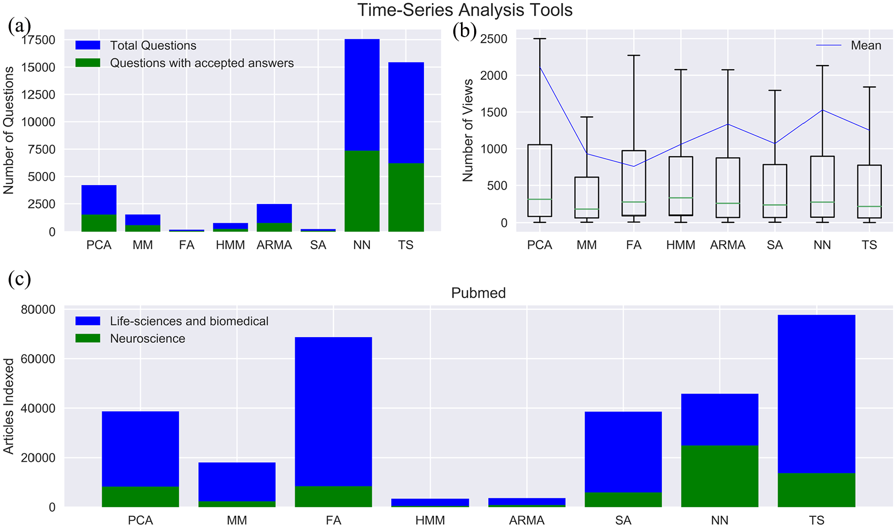
Comparison among time series tools. (a) In terms of questions asked and accepted answers, the neural network has recorded the most units, followed by PCA, ARMA-ARIMA, Markov models, HMM, Spectral, and Fourier analyses. Markov model, HMM, Spectral analysis, and Fourier series have applications in the frequency domain; thus, they exhibit significant but limited presence. Contrary to other tools, the neural network and PCA find application in different types of data and problem statements, ranging from classification to dimensionality reduction. However, an exception to this is ARMA-ARIMA models, which specifically deals with time series analysis and modeling. This may be a consequence of their straightforward concept and the vast amount of research available. Notably, almost all the tools have 40% accepted answers compared to the number of questions asked. (b) PCA has the highest number of views, followed by ARMA-ARIMA and neural networks, which has almost equal mean views; however, Fourier has the least mean views. In every time series tool, we observe that 50% of the questions have less than 300 views. The easy access to the internet and social connectivity has led to ample resources related to these topics, providing users with several alternatives. Among others, this could be the reason for a decline in mean viewership per question. (c) To our surprise, Fourier is the most used time series tool in biomedical and life science research, followed by PCA, Markov model, Neural network, and ARMA-ARIMA. Conversely, the neural network is the most used time series tool in neuroscience research, followed by PCA, Fourier, Spectral, Markov, and HMM.

Discussion

We have discussed seven classical time series tools in this work. Our focus has been the applications of these tools in biomedical, life sciences, and neuroscience. Due to the advent of internet technology and its explosive boom out in the last 2 decades, the exploitation of these tools increased globally. People all over the world, especially from China, Japan, USA, Canada, and some European countries have been early adopters of this technology. Our study quantified the use and evolution of these tools from several perspectives by analyzing the databases of SO, CV, and PubMed. It also sums up varied utilization all over the world, sharing ideas and giving a better idea of future scope.

Questions: Almost all the time series tools have marked their presence in 2008 or 2009 except ARMA-ARIMA and Fourier, which made their debut in 2011. Subsequently, an increment in the number of questions asked and accepted answers are observed. A few time series tools have shown a particular pattern or trend in their increment, whereas the trend in the rest of them was random. Most of them show a linear increment in questions asked (Figures 3 and 8), such as ARMA-ARIMA, whereas PCA and Spectral Analysis resemble a bell-curve (Figure 1). The growth in Markov and HMM has become constant after approximately 25 questions in 2012. For accepted answers, we observe that PCA, Spectral, and ARMA-ARIMA follow a rough linear increment with little or no fluctuations.

Conversely, Fourier transformation shows no trend and exhibits high fluctuations in the number of questions asked and accepted answers. Neural Network is the only time series tool that shows a polynomial growth in terms of questions asked and accepted answers. The neural network has always been a hot topic for research, and its application in various fields garnered questions over a range of 1K to 4K. Recent advancements in neural networks include a combination of CNN (Convolution Neural Network), RNN (Recurrent Neural Network) with artificial intelligence. This makes the neural network the most popular time series tool in SO and CV. The range of questions asked and accepted answers have been maximum for neural network followed by PCA and ARMA-ARIMA. In contrast, tools, such as Spectral, Markov, and HMM, gather 0 to 50 questions (Figures 5 -7).

Views: With the advent of time series tools in Q&A websites, they gain a considerable amount of high views per question and IQR. This suggests that IT-practitioners and researchers were looking for a platform to discuss these tools, and websites, such as SO and CV, facilitated them. Notably, for most of the time series tools, almost 75% of the questions have less viewership than the other 25%; thus, we observe that the mean views, that is, susceptible to extreme values, are generally above the third quartile. All the tools have witnessed a considerable decline in the mean viewership and IQR after 2011, which subsequently become negligible in the last few years. Fourier analysis, Spectral analysis, and Markov chain have very fluctuating mean viewership, whereas other tools are associated with an increment in the viewership at the beginning and a subsequent decline. Notably, a decline in mean views per question and subsequent increment in the number of questions suggest a nearly constant viewership, which is dispersed by the increment in the questions. In addition, it also suggests that the participation by the community is increasing, that is, more users are asking questions. Generally, views are in the range of 5K and 35K for PCA, which has fewer questions than the neural network; the mean viewership of the neural network lies in the range of 5K and 20K. Although some tools have fewer questions and accepted answers, they possess a considerable amount of views. For example, Spectral, HMM, and Markov have approximately 10 to 20 questions and approximately 30 to 40 accepted answers (Figures 5 -7); however, they have garnered approximately 5K as the highest mean views.

PubMed Analysis: The majority of the tools follow a non-decreasing trend in both biomedical and neuroscience domains. The increment in the use of these tools in neuroscience has not been substantial. However, the neural network shows peculiar polynomial growth in the life-science and biomedical domains. In addition, the neural network has witnessed substantial increment in terms of research indexed, especially related to neuroscience. There are a lot of research papers available regarding their applications in forecasting,^133,134 pattern and image recognition,^135,136 classification, and deep learning.⁴⁵ One such breakthrough occurred in 2011 when rectifier neurons¹³⁷ were presented as a better model for the biological neuron leading to equal or better performance. Except for HMM, all the other tools have a linearly increasing trend in biomedical and life sciences; however, the increment in neuroscience is gradual. Notably, although the tools like Spectral and Fourier analyses do not mark a significant presence in SO and CV, these tools have ample indexed papers in PubMed. It implies their considerable use in these domains. Fourier has been used in the analysis of signals from dynamic antral scintigraphy¹³⁸ for antral contraction rate estimation using empirical mode decomposition (EMD). Spectral analysis is used in the analysis of oscillations coming from the brain, which plays a key role in neural communication and computation. Often these oscillations are assumed to be sinusoidal. For example, in this study,¹³ non-sinusoidal features have been characterized, followed by providing crucial information to gain psychological features related to neural communication. In addition, PCA has abundant papers indexed; however, HMM and ARMA-ARIMA are the only tools with fewer indexed papers (Figure 9).

Most of these tools were used in combination with some other tools, not as an individual tool, especially Neural Networks and PCA, as they find application in both time and frequency domains.

Our analysis shows that a continuous rise in usage is not accompanied by a similar rise in questions with the accepted answer. Trends in the application of these tools from the biomedical and neuroscience perspective would introduce respective researchers to the current usage patterns of these resources. We hope this analysis would be useful for a wide range of professionals, ranging from IT-practitioners to Neuroscientists, in facilitating them with the right choice of tools. Also, it will guide to fill lacunae.

Supplemental Material

sj-docx-1-exn-10.1177_2633105520963045 – Supplemental material for Utilization of Time Series Tools in Life-sciences and Neuroscience

Supplemental material, sj-docx-1-exn-10.1177_2633105520963045 for Utilization of Time Series Tools in Life-sciences and Neuroscience by Harshit Gujral, Ajay Kumar Kushwaha and Sukant Khurana in Neuroscience Insights

Footnotes

Acknowledgements

Authors acknowledge sincere efforts of Akshat Garg (Jaypee Institute of Information Technology, Sector 128) for his help in the curation of this research.

Funding:

The author(s) received no financial support for the research, authorship, and/or publication of this article.

Declaration of conflicting interests:

The author(s) declared no potential conflicts of interest with respect to the research, authorship, and/or publication of this article.

Author Contributions

HG and AKK conducted the study and wrote the paper. HG scraped the data and created the visualizations. SK edited the paper. All three authors designed the study.

ORCID iDs

Harshit Gujral

Ajay Kumar Kushwaha

Sukant Khurana

Supplemental material

Supplemental material for this article is available online.

References

TC.

A review on time series data mining. Eng Appl Artif Intell. 2011;24:164-181.

Sejnowski

Churchland

Movshon

JA.

Putting big data to good use in neuroscience. Nat Neurosci. 2014;17:1440-1441.

Jorgenson

Newsome

Anderson

, et al. The BRAIN Initiative: developing technology to catalyse neuroscience discovery. Philos Trans R Soc Lond B Biol Sci. 2015;370:20140164.

Bullmore

Sporns

Complex brain networks: graph theoretical analysis of structural and functional systems. Nat Rev Neurosci. 2009;10:186-198.

Medaglia

Lynall

M-E

Bassett

DS.

Cognitive network neuroscience. J Cogn Neurosci. 2015;27:1471-1491.

Chatfield

What is the ‘best’method of forecasting?

J Appl Stat. 1988;15:19-38.

Jenkins

GM.

Some practical aspects of forecasting in organisations. J Forecast. 1982;1:3-21.

Makridakis

Anderson

Carbone

, et al. The accuracy of extrapolation (time series) methods: results of a forecasting competition. J Forecast. 1982;1:111-153.

Jolliffe

Cadima

Principal component analysis: a review and recent developments. Philos Trans A Math Phys Eng Sci. 2016;374:20150202.

10.

Keogh

Chakrabarti

Pazzani

Mehrotra

Dimensionality reduction for fast similarity search in large time series databases. Knowl Inf Syst. 2001;3:263-286.

11.

Keogh

A fast and robust method for pattern matching in time series databases. Proc WUSS. 1997;97:99.

12.

Debrégeas

Hébrail

. Interactive interpretation of Kohonen maps applied to curves. In: Agrawal

Stolorz

(eds) KDD’98: Proceedings of the Fourth International Conference on Knowledge Discovery and Data Mining. Palo Alto: AAAI Press; 1998:179-183.

13.

Keogh

Pazzani

. An enhanced representation of time series which allows fast and accurate classification, clustering and relevance feedback. In: KDD’98 Proceedings of the Fourth International Conference on Knowledge Discovery and Data Mining. New York: AAAI Press; 1998.

14.

Huang

Hegland

Data-mining massive time series astronomical data sets—a case study. In: Pacific-Asia Conference on Knowledge Discovery and Data Mining. Berlin, Heidelberg; April 1998.

15.

Das

Lin

Mannila

Renganathan

Smyth

. Rule discovery from time series. KDD.

16.

Freeman

Vladimirov

Kawashima

, et al. Mapping brain activity at scale with cluster computing. Nat Methods. 2014;11:941-950.

17.

Poldrack

Gorgolewski

KJ.

Making big data open: data sharing in neuroimaging. Nat Neurosci. 2014;17:1510-1517.

18.

Bassett

Sporns

Network neuroscience. Nat Neurosci. 2017;20:353-364.

19.

Broomhead

King

. Extracting qualitative dynamics from experimental data. Physica D. 1986a;20:217-236.

20.

Loska

Wiechuła

Application of principal component analysis for the estimation of source of heavy metal contamination in surface sediments from the Rybnik Reservoir. Chemosphere. 2003;51:723-733.

21.

Deluzio

Wyss

Zee

Costigan

Serbie

. Principal component models of knee kinematics and kinetics: normal vs. pathological gait patterns. Hum Mov Sci. 1997;16:201-17.

22.

Deluzio

Astephen

JL.

Biochemical features of gait waveform data associated with knee osteoarthritis: an application of principal component analysis. Gait Posture. 2007;25:86-93.

23.

Deluzio

Wyss

Costigan

Sorbie

Zee

Gait assessment in unicompartmental knee arthroplasty patients: principal component modelling of gait waveforms and clinical status. Hum Mov Sci. 1999;18:701-711.

24.

Ghil

Vautard

Interdecadal oscillations and the warming trend in global temperature time series. Nature. 1991;350:324-327.

25.

Giuliani

The application of principal component analysis to drug discovery and biomedical data. Drug Discov Today. 2017;22:1069-1076.

26.

Hanson

Sieverts

Vargis

Effect of principal component analysis centering and scaling on classification of mycobacteria from Raman spectra. Appl Spectrosc. 2017;71:1249-1255.

27.

Petrolis

Gintautas

Krisciukaitis

Multistage principal component analysis based method for abdominal ECG decomposition. Physiol Meas. 2015;36:329-340.

28.

Camacho

Picó Marco

JA.

Monitorización de procesos por lotes mediante PCA multifase. Rev Iberoam Autom In. 2010;3:78-91.

29.

Misra

Yue

Qin

Ling

Multivariate process monitoring and fault diagnosis by multi-scale PCA. Comput Chem Eng. 2002;26:1281-1293.

30.

Jia

Zhang

Jia

Zhang

Chen

Construction formula of biological age using the principal component analysis. Biomed Res Int. 2016;2016:4697017.

31.

Gløersen

Myklebust

Hallén

Federolf

. Technique analysis in elite athletes using principal component analysis. J Sports Sci. 2018;36:229-237.

32.

Palese

LL.

A random version of principal component analysis in data clustering. Comput Biol Chem. 2018;73:57-64.

33.

Jolliffe

IT.

Principal Component Analysis. 2nd ed. New York, NY: Springer-Verlag; 2002.

34.

Qin

Lei

Meng

. Research on forecasting the cost of residential construction based on PCA and LS-SVM. In: Proceedings of the International Conference on Electronics, Mechanics, Culture and Medicine (EMCM 2015). 2016; Atlantis Press. doi:10.2991/emcm-15.2016.17.

35.

Mazziotta

Pareto

. Composite index construction by PCA? No, thanks. 52 Riunione Scientifica SIEDS; May 2015; Ancona, Italy.

36.

Zhao

Liu

. The research of integrated dynamic analysis of metro project objectives based on PCA. In: Chen

Shen

Jiang

, eds. Applied Mechanics and Materials. Trans Tech Publications; 2014:2577-2580.

37.

Zurada

JM.

Introduction to Artificial Neural Systems (Vol. 8). St. Paul: West Publishing Company; 1992.

38.

Hassoun

. Fundamentals of Artificial Neural Networks. Cambridge, MA: MIT Press.

39.

Arbib

MA.

Warren McCulloch’s search for the logic of the nervous system. Perspect Biol Med. 2000;43:193-216.

40.

McCulloch

Pitts

A logical calculus of the ideas immanent in nervous activity. Bull Math Biophys. 1943;5:115-133.

41.

Jain

Mao

Mohiuddin

KM.

Artificial neural networks: a tutorial. Computer. 1996;29:31-44.

42.

Kim

Lee

WB.

Stock market prediction using neural networks with optimal feature transformation. Neural Comput Appl. 2004;13:255-260.

43.

Ngai

Wong

Chen

Sun

The application of data mining techniques in financial fraud detection: a classification framework and an academic review of literature. Decis Support Syst. 2011;50:559-569.

44.

Estévez

Held

Perez

CA.

Subscription fraud prevention in telecommunications using fuzzy rules and neural networks. Expert Syst Appl. 2006;31:337-344.

45.

LeCun

Bengio

Hinton

Deep learning. Nature. 2015;521:436-444.

46.

Morphy

. What is a neural network and how are businesses using them? https://www.cmswire.com/digital-experience/what-is-a-neural-network-and-how-are-businesses-using-it/. 2018.

47.

Hinton

Deng

, et al. Deep neural networks for acoustic modeling in speech recognition: the shared views of four research groups. IEEE Signal Process Mag. 2012;29:82-97.

48.

Auld

Moore

Gull

SF.

Bayesian neural networks for internet traffic classification. IEEE Trans Neural Netw Learn Syst. 2007;18:223-239.

49.

Lippmann

RP.

Pattern classification using neural networks. IEEE Commun Mag. 1989;27:47-50.

50.

Tajbakhsh

Shin

Gurudu

, et al. Convolutional neural networks for medical image analysis: full training or fine tuning? IEEE Trans Med Imaging. 2016;35:1299-1312.

51.

Khan

Wei

Ringner

, et al. Classification and diagnostic prediction of cancers using gene expression profiling and artificial neural networks. Nat Med. 2001;7:673-679.

52.

Palmer

Montano

Sesé

Designing an neural network for forecasting tourism time series. Tour Manag. 2006;27:781-790.

53.

Abdel-Aal

RE.

Univariate modeling and forecasting of monthly energy demand time series using abductive and neural networks. Comput Ind Eng. 2008;54:903-917.

54.

Ramachandran

Hong

Sime

Wilson

GA.

Diabetic retinopathy screening using deep neural network. Clin Exp Ophthalmol. 2018;46:412-416.

55.

Cheng

Yang

Sheng

. Colorization using neural network ensemble. IEEE Trans Image Process 26:5491-5505.

56.

Xie

Wang

Zhang

, et al. Bidirectional Recurrent Neural Network and Convolutional Neural Network (BiRCNN) for ECG beat classification. In: 2018 40th Annual International Conference of the IEEE Engineering in Medicine and Biology Society (EMBC). IEEE: Honolulu, HI; 2018:2555-2558.

57.

Han

Hou

Qiao

JF.

An adaptive-PSO-based self-organizing RBF neural network. IEEE Trans Neural Netw Learn Syst. 2016;29:104-117.

58.

Zhang

Zhong

Smith

Cellular neural network modelling of soft tissue dynamics for surgical simulation. Technol Health Care. 2017;25:337-344.

59.

Box

GEP

Jenkins

. Time Series Analysis: Forecasting and Control, Revised ed. San Francisco, CA: Holden-Day.

60.

Whittle

Hypothesis Testing in Time Series Analysis. New York, NY: Hafner Publishing Company; 1951.

61.

Yule

GU.

Why do we sometimes get nonsense-correlations between time series? a study in sampling and the nature of time series. J R Stat Soc. 1926;89:1-64.

62.

Wold

A Study in the Analysis of Stationary Time Series. [Doctoral thesis]. Stockholm: Almgrist & Wiksell; 1938.

63.

Box

GEP

Pierce

DA.

Distribution of residual autocorrelations in autoregressive-integrated moving average time series models. J Am Stat Assoc. 1970; 65:1509-1526.

64.

McLeod

WK.

Diagnostic checking ARMA time series models using squared-residual autocorrelations. J Time Ser Anal. 1983;4:269-273.

65.

Hurvich

Tsai

C-L.

Regression and time series model selection in small samples. Biometrika. 2015;76:297-307.

66.

Zhang

GP.

Time series forecasting using a hybrid ARMA and neural network model. Neurocomputing. 2001;50:159-175.

67.

Wei

Jiang

Liang

, et al. Application of a combined model with autoregressive integrated moving average (ARIMA) and generalized regression neural network (GRNN) in forecasting hepatitis incidence in Heng County, China. PLoS One. 2016;11:e0156768.

68.

Mekparyup

Saithanu

Combining seasonal ARIMA model and adjusted Tukey’s control chart with interpretation rules for monitoring epidemic of dengue hemorrhagic fever. Glob J Pure Appl Math. 2015;11:2151-2154.

69.

Zhang

Wang

Qin

Wang

Forecasting of particulate matter time series using wavelet analysis and wavelet-ARMA/ARIMA model in Taiyuan, China. J Air Waste Manage Assoc. 2017;67:776-788.

70.

Ebrahimi

Hamdami

Moemenbellah-Fard

Jahromi

. Predictive determinants of scorpion stings in a tropical zone of south Iran: use of mixed seasonal autoregressive moving average model. J Venom Anim Toxins Incl Trop Dis. 2017;23:39.

71.

Chan

MF.

Predictive time-series modeling using neural networks for Linac beam symmetry: an empirical study. Ann N Y Acad Sci. 2017;1387:84-94.

72.

Teng

Xie

, et al. Dynamic forecasting of Zika epidemics using Google Trends. PLoS One. 2017;12:e0165085.

73.

Liu

Hoi

Zhao

Sun

. Online ARIMA algorithms for time series prediction. In: AAAI-16: Proceedings of Thirtieth AAAI Conference on Artificial Intelligence; February 12-17, 2016; AAAI Press: Phoenix, Arizona.

74.

Petrevska

Predicting tourism demand by ARIMA models. Economic research-Ekonomska istraživanja. 2017;30:939-950.

75.

Heng

WANG

Zhang

Yang

. The application of ARIMA model in the project of China Zun Tower. DEStech Trans Eng Technol Res. 2017; (icmme).

76.

Mondal

Shit

Goswami

Study of effectiveness of time series modeling (ARIMA) in forecasting stock prices. Int J Comput Sci Eng Appl. 2014;4:13-29.

77.

Chujai

Kerdprasop

. Time Series Analysis of Household Electric Consumption with ARMA and ARMA Models. In: Proceedings of the International MultiConference of Engineers and Computer Scientists (IMECS). Hong Kong; 13-15 March 2013.

78.

Iwok

IA.

Handling seasonal autoregressive integrated moving average model with correlated residuals. Am J Math Stat. 2017;7:1-6.

79.

Oleg Grachev (2017). Application of Time Series Models (ARMA, GARCH, and ARMA-GARCH) for Stock Market Forecasting. [Dissertation/Thesis]. Northern Illinois University; 2017.

80.

Ariyo

Adewumi

Ayo

CK.

Stock price prediction using the ARIMA model. UKSim-AMSS 16th International Conference on Computer Modelling and Simulation; March 26-28, 2014; Cambridge.

81.

Dickey

Pantula

SG.

Determining the order of differencing in autoregressive processes. J Bus Econ Stat. 1987;5:455-461.

82.

Smyth

. Deformable MARKOV model templates for time series pattern matching. In: Proceedings of the Sixth ACM SIGKDD International Conference on Knowledge Discovery and Data Mining; 2000; New York, NY.

83.

Zeger

Qaqish

MARKOV regression models for time series: a quasi-likelihood approach. Biometrics. 1988;44:1019-1031.

84.

Cox

. The Analysis of Binary Data. 2nd ed. London: Chapman and Hall.

85.

Lebenbaum

Cheng

de Oliveira , et al. Evaluating the cost effectiveness of a suicide prevention campaign implemented in Ontario, Canada. Appl Health Econ Health Policy. 2020;18:189-201.

86.

Simon

Harmer

Kingslake

Dawson

Dourish

Goodwin

GM.

Value of monitoring negative emotional bias in primary care in England for personalised antidepressant treatment: a modelling study. Evid Based Ment Health. 2019;22:145-152.

87.

Slade

Daly

Mavranezouli

, et al. Primary surgical management of anterior pelvic organ prolapse: a systematic review, network meta-analysis and cost-effectiveness analysis. BJOG. 2019;127:18-26.

88.

Bargiela

Bianchi

Westover

, et al. Selection of first-line therapy in multiple sclerosis using risk-benefit decision analysis. Neurology. 2017;88:677-684.

89.

Liegeois

Laumann

Snyder

Zhou

Yeo

BT.

Interpreting temporal fluctuations in resting-state functional connectivity MRI. Neuroimage. 2017:163:437-455.

90.

Zhou

Wang

Zhong

Tan

A Markov chain based demand prediction model for stations in bike sharing systems. Math Probl Eng. 2018;2018:8028714.

91.

Touron

Modeling rainfalls using a seasonal hidden Markov model. arXiv preprint arXiv:1710.08112. 2017.

92.

Choo

Tong

Zhang

Recent applications of hidden Markov models in computational biology. Genomics Proteomics Bioinformatics. 2004;2:84-96.

93.

Krogh

Larsson

von Heijne

, et al. Predicting transmembrane protein topology with a hidden MARKOV Model: application to complete genomes. J Mol Biol. 2001;305:567-580.

94.

Yamato

Ohya

Ishii

Recognizing human action in time-sequential images using hidden Markov model. In: Proceedings 1992 IEEE Computer Society Conference on Computer Vision and Pattern Recognition. 15-18 June, 1992; Champaign, IL: IEEE.

95.

Bahi

Brown

de Souza

Mercer

. Maximum Mutual Information Estimation of Hidden Markov Model Parameters for Speech Recognition. In: ICASSP ’86. IEEE International Conference on Acoustics, Speech, and Signal Processing. 7-11 April, 1986; Tokyo: IEEE.

96.

Varga

Moore

. Hidden Markov model decomposition of speech and noise. In: International Conference on Acoustics, Speech, and Signal Processing. 3-6 April, 1990; Albuquerque, NM: IEEE.

97.

Fine

Singer

Tishby

The hierarchical hidden MARKOV model: analysis and applications. Mach Learn. 1998;32:41-62.

98.

Rybert Sipos

Parallel stratified MCMC sampling of AR-HMMs for stochastic time series prediction/Ed. CH Skiadas. In: Proceedings of the 4th Stochastic Modeling Techniques and Data Analysis International Conference with Demographics Workshop (SMTDA 2016). Valletta, Malta: University of Malta; 2016:361-364.

99.

Vogl

Futschik

. Hidden Markov models in biology. In: Data Mining Techniques for the Life Sciences. New York: Humana Press; 2010:241-253.

100.

Vijayabaskar

. Introduction to hidden Markov models and its applications in biology. In: Hidden Markov Models. New York: Humana Press; 2017:1-12.

101.

Asgari

Adams

Kasprowicz

Czosnyka

Smielewski

Ercole

Feasibility of hidden Markov models for the description of time-varying physiologic state after severe traumatic brain injury. Crit Care Med. 2019;47: e880-e885.

102.

Zhang

Cai

Zhang

, et al. Estimating Dynamic Functional Brain cConnectivity with a Sparse Hidden Markov Model. IEEE Trans Med Imaging. 2019;39:488-498.

103.

Park

Kotzias

Kuo

, et al. Detecting conversation topics in primary care office visits from transcripts of patient-provider interactions. JAMA. 2019;26:1493-1504.

104.

Sgouralis

Pressé

An introduction to infinite HMMS for single-molecule data analysis. Biophys J. 2017;112:2021-2029.

105.

Ghosh

Cao

Ramamohanarao

Septic shock prediction for ICU patients via coupled HMM walking on sequential contrast patterns. J Biomed Inform. 2017;66:19-31.

106.

Domingos

. The Master Algorithm: How the quest for the Ultimate Learning Machine will Remake Our World. New York: Basic Books; 2015.

107.

Ghassempour

Girosi

Maeder

Clustering multivariate time series using hidden Markov models. Int J Environ Res Public Health. 2014;11:2741-2763.

108.

Sampathkumar

Chen

Luo

Mining adverse drug reactions from online healthcare forums using hidden Markov model. BMC Med Inform Decis Mak. 2014;14:91.

109.

Cao

. A high-order hidden Markov model for emotion detection from textual data. In: Pacific Rim Knowledge Acquisition Workshop. Springer, Berlin, Heidelberg; 2012:94-105.

110.

Lagrange

JL.

Réflexions sur la résolution algébrique des équations. New York: Basic Books; 1770.

111.

Deeming

TJ.

Fourier analysis with unequally-spaced data. Astrophys Space Sci. 1975;36:137-158.

112.

Beckner

Inequalities in Fourier analysis. Ann Math. 1975;102:159-182.

113.

Allen

Rabiner

LR.

A unified approach to short-time Fourier analysis and synthesis. Proc IEEE. 1977;65:1558-1564.

114.

Ablowitz

Kaup

Newell

Segur

The inverse scattering transform-Fourier analysis for nonlinear problems. Stud Appl Math. 1974;53:249-315.

115.

El Hady

WEA

Mohamed

Soliman

OAEA

EL-Sabbagh

HM.

In vitro–in vivo evaluation of chitosan-PLGA nanoparticles for potentiated gastric retention and anti-ulcer activity of diosmin. Int J Nanomed. 2019;14:7191.

116.

Yokel

Hancock

Cherian

, et al. Simulated biological fluid exposure changes Nanoceria’s surface properties but not its biological response. Eur J Pharm Biopharm. 2019;144:252-265.

117.

Lupaescu

Humelnicu

Petre

Ciobanu

Drochioiu

Direct evidence for binding of aluminum to NAP anti-amyloid peptide and its analogs. Eur J Mass Spectrom. 2020;26:106-116.

118.

Rodríguez-Félix

Del-Toro-Sánchez

Javier Cinco-Moroyoqui

, et al. Preparation and characterization of quercetin-loaded zein nanoparticles by electrospraying and study of in vitro bioavailability. J Food Sci. 2019;84:2883-2897.

119.

Bond

Correia

Sauvage

Neichel

Fusco

Iterative wave-front reconstruction in the Fourier domain. Opt Express. 2017;25:11452-11465.

120.

Teixeira

Gouveia

Duarte

, et al. Regular exercise participation contributes to better proteostasis, inflammatory and vasoactive profiles in patients with hypertension. Am J Hypertens. 2020;33:119-123.

121.

Diaz

del Busto

Escudero

Pérez

Clock genes disruption in the intensive care unit. J Intensive Care Med. 2019:885066619876572.

122.

Abdo

Lamare

Fernandez

Bentourkia

MH.

Analysis of hypoxia in human glioblastoma tumors with dynamic 18F-FMISO PET imaging. Australas Phys Eng Sci Med. 2019;42:981-993.

123.

Martins

Westerfield

Lopes

Maruta

Gil-da-Costa

Brain state monitoring for the future prediction of migraine attacks. Cephalalgia. 2020;40:255-265.

124.

Joo

Han

Lee

Jang

Kang

Woo

Spectral analysis of acceleration data for detection of generalized tonic-clonic seizures. Sensors. 2017;17:481.

125.

Hossen

Barhoum

Jaju

, et al. Identification of patients with preeclampsia from normal subjects using wavelet-based spectral analysis of heart rate variability. Technol Health Care. 2017;25:641-649.

126.

Ralbovsky

Halámková

Wall

Anderson-Hanley

Lednev

IK.

Screening for Alzheimer’s disease using saliva: a new approach based on machine learning and Raman hyperspectroscopy. J Alzheimers Dis (Preprint). 2019;71:1351-1359.

127.

Leise

TL.

Analysis of nonstationary time series for biological rhythms research. J Biol Rhythms. 2017;32:187-194.

128.

McCullough

Sakellariou

Stemler

Small

Regenerating time series from ordinal networks. Chaos. 2017;27:035814.

129.

Wong

Tashiro

Kuhara

Aburatani

Elucidation of the sequential transcriptional activity in Escherichia coli using time-series RNA-seq data. Bioinformation. 2017;13:25-30.

130.

Grootswagers

Wardle

Carlson

TA.

Decoding dynamic brain patterns from evoked responses: a tutorial on multivariate pattern analysis applied to time series neuroimaging data.J Cogn Neurosci. 2017;29:677-697.

131.

Gupta

Jansen

Hofman

, et al. Wavelet entropy of BOLD time series: an application to Rolandic epilepsy. J Magn Reson Imaging. 2017;46:1728-1737.

132.

Fraedrich

Estimating dimensions of weather and climate attractors. J Atmos Sci. 1986;43:419–432.

133.

Hippert

Pedreira

Souza

RC.

Neural networks for short-term load forecasting: a review and evaluation. IEEE Trans Power Syst. 2001;16:44-55.

134.

Vellido

Lisboa

Vaughan

Neural networks in business: a survey of applications (1992–1998). Expert Syst Appl. 1999;17:51-70.

135.

Zhang

Ren

Sun

. Deep residual learning for image recognition. In: Proceedings of the IEEE Conference on Computer Vision and Pattern Recognition. 2016; Las Vegas, NV: IEEE:770-778.

136.

Ronneberger

Fischer

Brox

. U-net: Convolutional networks for biomedical image segmentation. In: International Conference on Medical Image Computing and Computer-Assisted Intervention. NY: Springer, Cham; 234-241.

137.

Glorot

Bordes

Bengio

. Deep sparse rectifier neural networks. In: Proceedings of the Fourteenth International Conference on Artificial Intelligence and Statistics; 2011;15:315-323. http://proceedings.mlr.press/v15/glorot11a/glorot11a.pdf

138.

Ngamsirijit

Jarumaneeroj

Chaiwatanarat

Rakvongthai

. Analysis of dynamic antral scintigraphy using empirical mode decomposition. In:2017 39th Annual International Conference of the IEEE Engineering in Medicine and Biology Society (EMBC). Seogwipo, South Korea, IEEE; 2017:2932-2935. doi:10.1109/EMBC.2017.8037471.

139.

Baum

Petrie

Soules

Weiss

A maximization technique occurring in the statistical analysis of probabilistic functions of Markov chains. Ann Math Statist. 1970;41:164-171.

140.

Broomhead

King

. On the qualitative analysis of experimental dynamical systems. In: Sarkar

, ed. Nonlinear phenomena and chaos. Bristol: Adam Hilger; 1986b:113-144.

141.

Vautard

Ghil

Singular spectrum analysis in nonlinear dynamics, with applications to paleoclimatic time series. Physica D. 1989;35:395-424.

142.

Vautard

Yiou

Ghil

Singular-spectrum analysis: a toolkit for short, noisy chaotic signals. Physica D. 1992; 58:95-126.

143.

Alonso

Del Castillo

Pintado

Application of singular spectrum analysis to the smoothing of raw kinematic signals. J Biomech. 2005;38:1085-1092.

144.

Oropeza

Sacchi

Simultaneous seismic data denoising and reconstruction via multichannel singular spectrum analysis. Geophys 2011;76:V25-V32.

145.

Hassani

Zhigljavsky

Singular spectrum analysis: methodology and application to economics data. J Syst Sci Complex. 2009;22:372-394.

Supplementary Material

Please find the following supplemental material available below.

For Open Access articles published under a Creative Commons License, all supplemental material carries the same license as the article it is associated with.

For non-Open Access articles published, all supplemental material carries a non-exclusive license, and permission requests for re-use of supplemental material or any part of supplemental material shall be sent directly to the copyright owner as specified in the copyright notice associated with the article.

0.00 MB

0.19 MB