
Abstract
In a real-world observational data analysis setting, guessing the true model specification can be difficult for an analyst. Unfortunately, correct model specification is a core assumption for treatment effect estimation methods such as propensity score methods, G-computation, and regression techniques. Targeted maximum likelihood estimation (TMLE) is an alternative method that allows the use of data-adaptive and machine learning algorithms for model fitting. TMLE therefore does not require strict assumptions about the model specification but preserves the validity of the inference. Multiple studies have shown that TMLE outperforms other methods in certain real-world settings, making it a useful and potentially superior algorithm for causal inference. However, there is a lack of accessible resources for practitioners to understand the implementation. Hence the TMLE framework is the least-used method by practitioners in epidemiology literature. Recently a few accessible articles have been published, but they focus only on binary outcomes and demonstrations are done mainly with simulated data. This paper aims to fill the gap in the literature by providing a step-by-step TMLE implementation guide for a continuous outcome, using an openly accessible clinical dataset.
Introduction
The goal of causal inference is to extract the amount of change in the outcome caused exclusively by a change in the treatment of interest. This causal effect can be formally defined based on the counterfactual framework established by Rubin, discussed in detail later. 1 In 2006, Van der Laan and Rubin developed targeted maximum likelihood estimation (TMLE), 2 a promising causal inference method. TMLE is different from traditional methods in that it uses estimates of both the treatment-generating mechanism (propensity score model) and the outcome-generating mechanism to estimate the average treatment effect. The use of both of these models has a special advantage because TMLE is doubly robust, meaning it provides a consistent estimator if either the exposure or outcome model is correctly specified. 3 TMLE has been shown to outperform inverse probability of treatment weighting (IPTW) and G-computation methods (discussed later), particularly when model misspecification is likely.3–8 Despite its gaining recognition in the statistical sciences, there is a shortage of resources accessible to practitioners who could benefit from using TMLE in real-world scenarios. In particular, though Luque-Fernandez et al. provide a well-written guide to TMLE for a binary outcome, 5 such a tutorial for Gruber and van der Laan’s method for a continuous outcome has yet to be published. 6 The steps are similar to those for a binary outcome, but there is little easily understandable high-level literature on the differences. Continuous outcomes are widespread in epidemiology, though they are often dichotomized for ease of analysis and to correlate directly with care decisions. The dichotomization of a continuous outcome, however, creates several problems. Firstly, it reduces the statistical power of the analysis since we are losing information about the outcome variable. 9 Secondly, the calculated measures of association change with the cut point used to dichotomize the variable and the underlying distribution. 10 Due to these risks, leaving the variable as a continuous outcome is often beneficial. The understanding of TMLE in the continuous outcome setting is therefore especially important. Additionally, previous guides on the implementation of TMLE have primarily focused on simulated data.5,11 This article aims to demonstrate the steps of TMLE to estimate the treatment effect using a real-world, openly accessible dataset to give practitioners a sense of how this method works in practice. 12 We also explain the related approaches in an organized way, so that readers understand the difference between the commonly used methods and TMLE.
Methods
Rubin’s causal framework
Essentially, Rubin’s framework states that if in a study with a binary treatment
Assumptions
To estimate the counterfactuals described in Rubin’s causal framework, and label the resulting treatment effect as causal, there are several assumptions we have to make.
14
1. Conditional exchangeability: the conditional probability of receiving treatment depends only on the measured covariates. In other words, the unmeasured factors that affect the outcome are distributed equally between the treated and untreated groups, conditional on measured confounders.
13
2. Positivity: for each combination of covariate levels, there must be a positive probability of each treatment condition (treated and untreated). The outcome of one subject may not depend on the treatment any other subject received.
13
3. Consistency: the treatment must be well-defined so that there is no ambiguity about dosage, length of treatment, or other factors that could cause the level of exposure to differ between subjects. If we know the exposure is well-defined, we can assume a subject’s observed outcome will be equal to their corresponding counterfactual outcome given their observed exposure history.
15
G-computation method
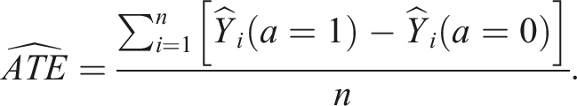
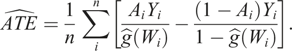
Under the above assumptions, the average treatment effect (ATE) can be defined as the average outcome under treatment minus the average outcome under no treatment.

One of the methods commonly used to estimate the treatment effect using counterfactual outcomes is the G-computation method. It is based on modelling the outcome and uses linear regression models to predict the outcome for each subject under each treatment. All covariates, represented here as the matrix

For instance, for a binary treatment
G-computation performs poorly under model misspecification and requires the use of bootstrap sampling, a tedious resampling technique, to calculate confidence intervals. 5
Inverse probability of treatment weighting (IPTW) method
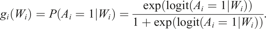
Another common approach to estimate the treatment effect is the inverse probability of treatment weighting (IPTW), a propensity score-based estimation method that models the treatment-generating mechanism. The propensity score is the conditional probability of this observation being assigned the treatment given all measured covariates. The propensity score model, also called the treatment model, is typically estimated through logistic regression (shown for data with
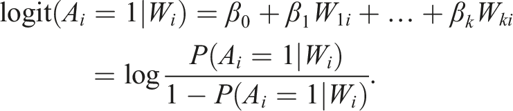
The propensity scores are then:
The weights for the average treatment effect (ATE) are calculated as follows:
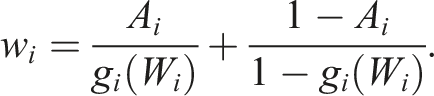
Those who were very likely to receive the treatment and did receive the treatment will be weighted less heavily than the treated who were unlikely to receive treatment, artificially balancing the distribution of covariates between the two groups.
19
The weights for each observation are multiplied by the corresponding outcome. When a particular observation is treated (
IPTW estimates can be unstable with a high variance if there are propensity score values close to 0, leading to large weights. The method is also sensitive to model misspecification, especially with a large number of variables. 5
TMLE
Targeted maximum likelihood estimation (TMLE) combines an outcome model based on the G-computation framework with an exposure model based on IPTW to estimate the parameter of interest. 20 Incorporating both models makes this method doubly robust, so the estimate of our parameter of interest will be consistent if either the outcome or exposure model is correctly specified. A consistent estimator essentially means the estimate gets closer and closer to the true value as the sample size increases. 11 If both models are correctly specified, the estimate will be efficient, meaning a smaller sample size is required for a narrow confidence interval than if one method were misspecified. 3 A further benefit of TMLE is that it allows for the use of machine learning algorithms in generating both the treatment (propensity score) and outcome models. This is not possible in the pure propensity score and G-computation methods because the sampling distribution of the estimate resulting from the use of machine learning to directly estimate the treatment effect generally does not approximate a known distribution. 21 Usually, a standard regression using maximum likelihood estimation will give an estimate that follows an approximate normal distribution, assuming the model was correctly specified. Statistical inference such as standard errors and confidence intervals are then straightforward to calculate. By contrast, if machine learning is used directly in a model from which the estimate is extracted directly, statistical inference is not straightforward since the estimator does not follow a known distribution. 21 TMLE, on the other hand, uses machine learning only in intermediary steps, rather than to estimate the parameter of interest directly. The sampling distribution of our estimate is therefore approximately normal and statistical inference is still straightforward. Data-adaptive modelling allows TMLE to require more relaxed assumptions about the data structure than other methods, aiding in the minimization of bias and the construction of an efficient estimator. 3 It has been shown that doubly robust estimators using machine learning, such as TMLE, outperform singly robust estimators using machine learning, such as IPTW. 22
For a binary outcome, as shown in previous tutorials, 5 the process of implementing TMLE is fairly straightforward. Since the range of a binary outcome is completely predictable, it is guaranteed that all our estimated outcomes will be inside the 0-1 range. If the same approach is used for a continuous outcome, the assumption that the modeled outcomes lie within the range of the true distribution may not hold. 6 Predicted outcomes outside the true distribution’s range can result in increased bias and variance in the estimator, particularly in sparse data settings.3,6 In 2010, Susan Gruber and Mark J. van der Laan suggested a slightly modified approach to TMLE with a bounded continuous outcome. 6 They suggest the same approach to be used for continuous outcomes where the bounds are not known a priori by setting the minimum and maximum of the sample outcome as the bounds. This approach uses a logistic fluctuation function rather than the linear function typically used for continuous outcomes.
SuperLearner
In this tutorial we apply SuperLearner as the machine learning algorithm to generate the treatment and outcome models. 23 SuperLearner is an ensemble machine learning technique that can either (i) select from or (ii) combine different machine learning techniques into one “super learner” to make outcome predictions based on a set of given covariates. In the selection version, SuperLearner uses cross-validation to select the best machine learning algorithm for the given dataset from a list of candidate algorithms provided by the user. The combination version uses cross-validation to select the best possible linear combination of the candidate algorithms provided. 23 The SuperLearner package in R implements versions of both, with a default list of candidate machine learning algorithms. 24 SuperLearner will always be at least as accurate as the best algorithm included in the set of algorithms it can draw from. 24 It is, therefore, the recommended approach for constructing both the treatment and outcome models in TMLE. 3
Motivating example: Right heart catheterization
This guide will go through a step-by-step example using the right heart catheterization (RHC) dataset. This dataset of 5735 adult patients was used by Connors et al. in their 1996 study of the effectiveness of RHC in the initial care of critically ill patients. 12 Included patients were receiving care in an intensive care unit (ICU) for one of nine prespecified disease categories and the group was selected to have a total 6-months mortality of 50%. The original study used propensity score matching to analyze the effect of receiving RHC in the first 24 h of care in the ICU on survival time, cost of care, intensity of care, and length of stay in the ICU and hospital. The variables to include in the propensity score were chosen with the expertise of a panel of four intensivists and three cardiologists. In this example, we focus on the continuous outcome of length of stay. The study by Connors et al. reported an increase of 1.8 days in length of stay for patients who received RHC compared to those who did not. The code we used to prepare the dataset can be found in Box 14 in the supplementary materials.
TMLE steps
Targeted maximum likelihood estimation (TMLE) steps when the outcome of interest is continuous.
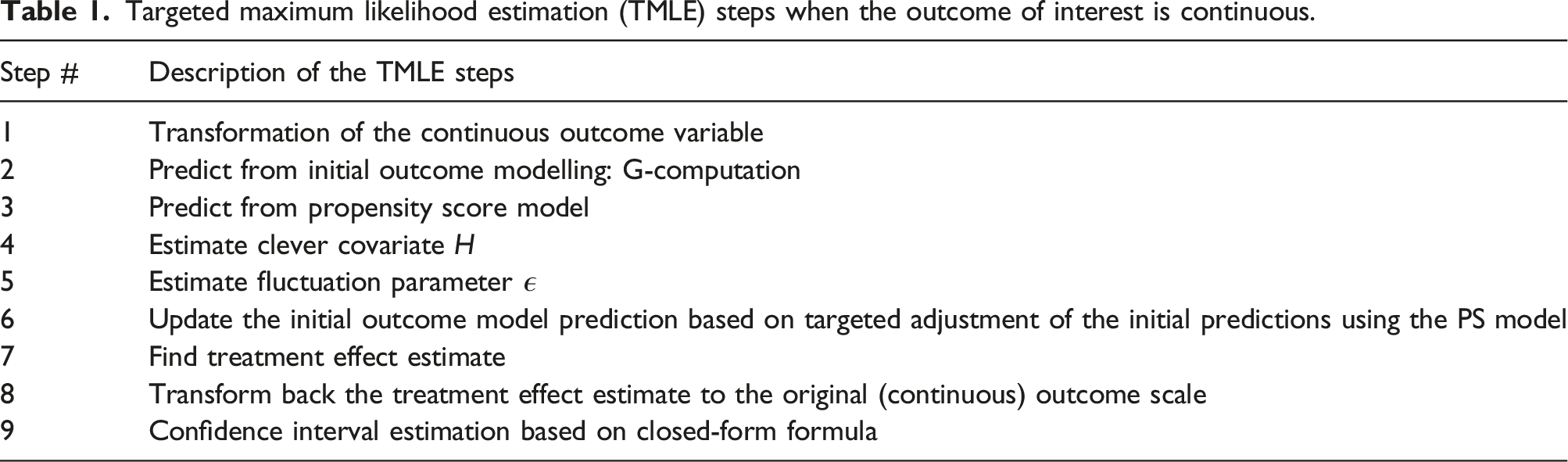
Step-by-Step Analysis
Step 1: Transformation of the continuous outcome variable
With a binary outcome, our initisal crude estimate of the treatment effect 
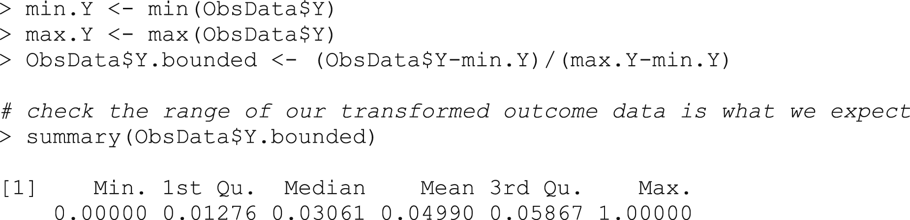
A key step in TMLE for a continuous outcome is to transform our outcome 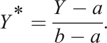
The R code for the transformation of 
The parameter of interest on the transformed scale relates to our original parameter of interest 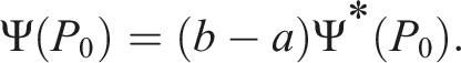
If our outcome is technically unbounded, we can use the minimum and maximum outcomes found in our sample data as
Box 1 – Transforming the outcome Y to the scale [0,1]
Step 2: Predict from initial outcome modelling: G-computation
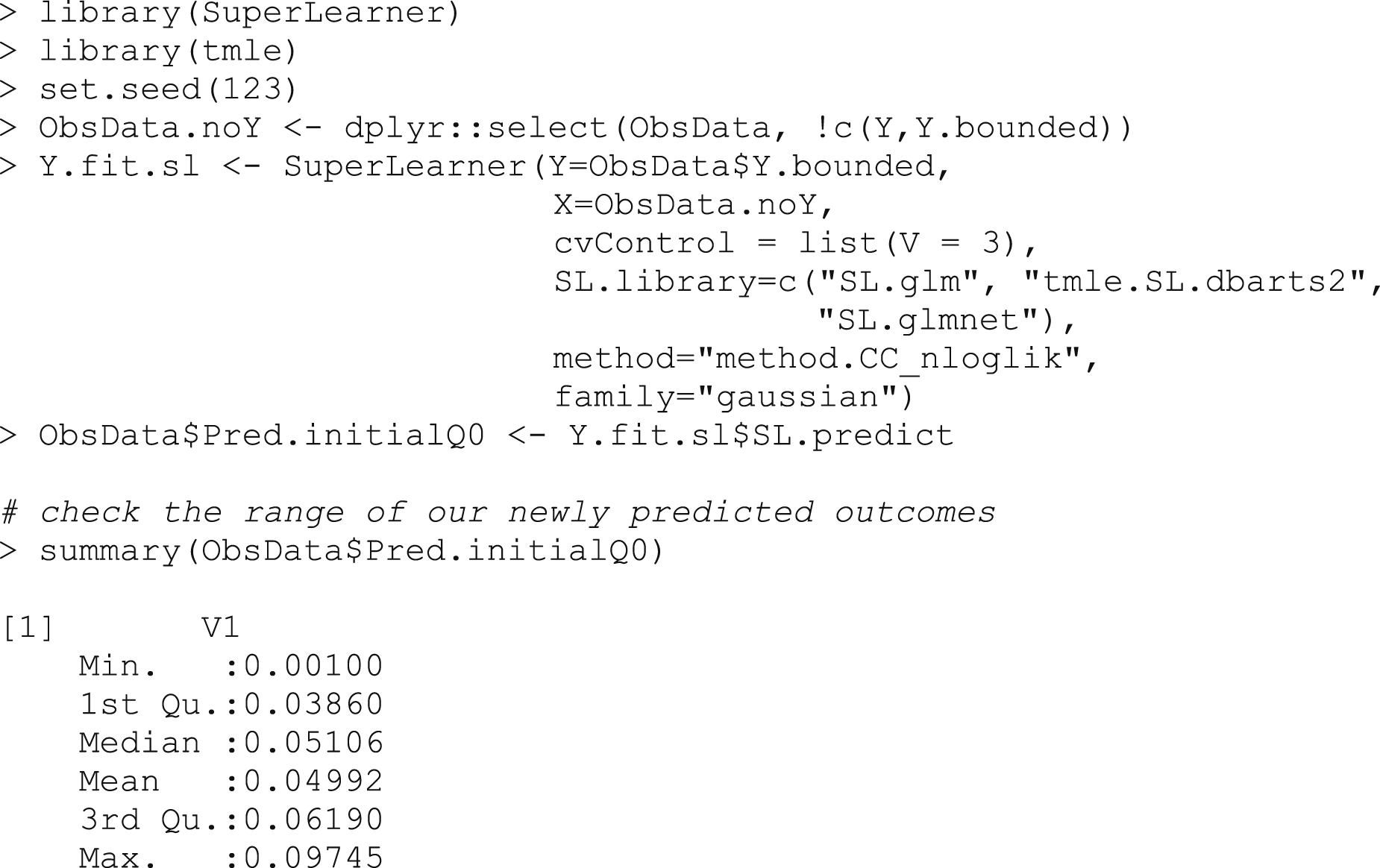
In the first stage of TMLE, we need to calculate our starting point. This means following the G-computation framework to find an initial crude estimate of the ATE. The use of data-adaptive methods such as SuperLearner is recommended for this step, since they are less likely to result in model misspecification than parametric methods since they make no a priori assumptions about the data model. In TMLE, unlike singly robust methods such as propensity score methods, the use of machine learning algorithms does not come at the cost of interpretability. 3
Using the SuperLearner package, we can fit an initial model for the outcome 
Box 2 – Fitting the initial outcome model using SuperLearner and making predictions for observed treatment assignments
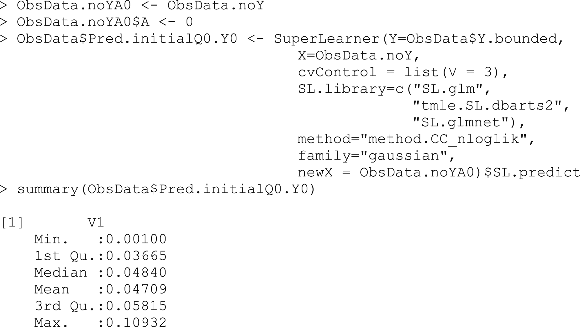
As well as predicting the outcome under treatment received, we also predict the outcomes for each subject under each theoretical treatment, regardless of what treatment they truly received (Box 3a,3b).
Box 3a – Making predictions
for the counterfactual outcome, assigning all treatments to A = 1

Box 3b – Making predictions
for the counterfactual outcome, assigning all treatments to A = 0
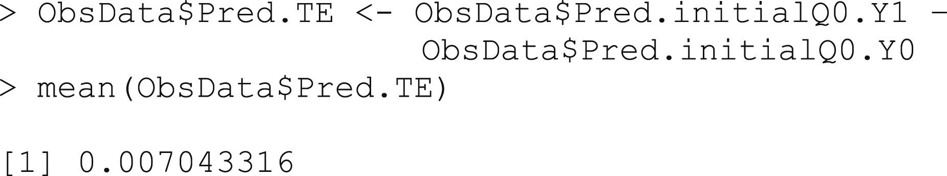
These values,
Box 4 – Calculating the crude ATE estimate using counterfactual outcome predictions
Step 3: Predict from propensity score model
The next step is to construct the propensity score model to be used in our calculation of the so-called clever covariates and a fluctuation parameter 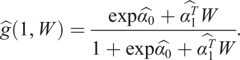
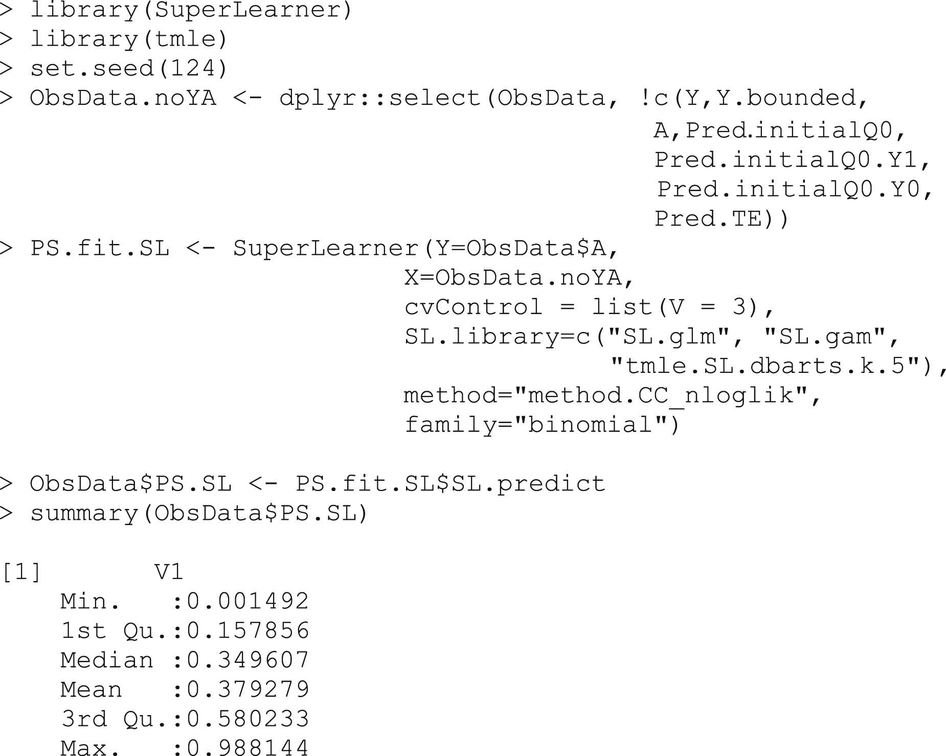
However, it is again recommended to use a SuperLearner to construct the propensity score model, then use the fitted model to predict the probabilities
Box 5 – Constructing the propensity score models and extracting the propensity scores through prediction
Step 4: Estimate clever covariate
To update our estimate, we define the parametric submodel: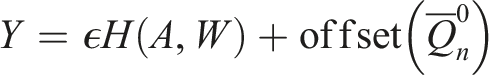
We set
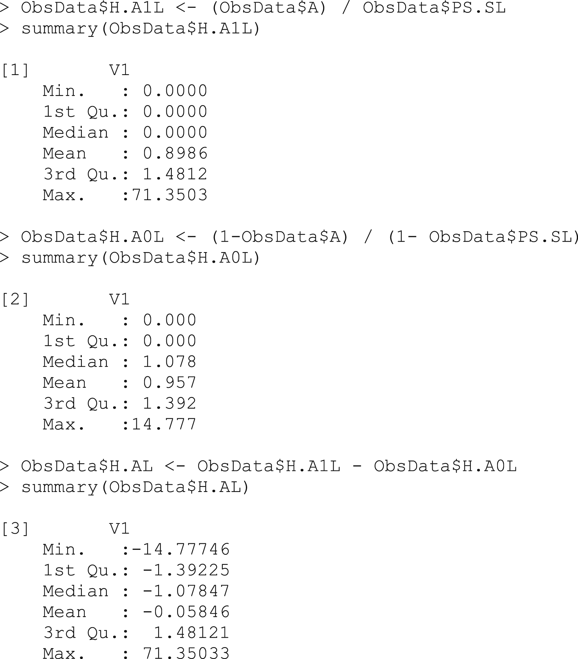
The clever covariate
Box 6 – Using the propensity scores to calculate the clever covariates
The clever covariate allows us to target the update of our estimate towards the true value of the parameter we are interested in. The weights are higher for the cases with an unlikely treatment-covariate combination, since they are underrepresented in the dataset compared to the ideal scenario in which the groups would be completely comparable. The weighted treated and untreated observations will thus be artificially balanced in terms of all the other covariates.
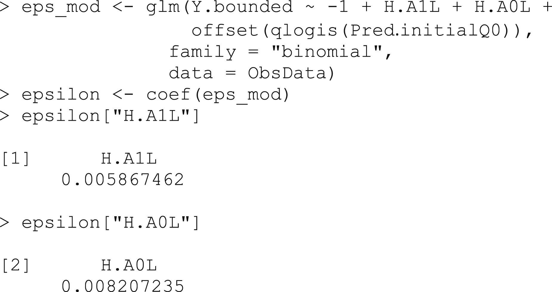
Step 5: Estimate fluctuation parameter
We also need to estimate our fluctuation parameter. The fluctuation parameter 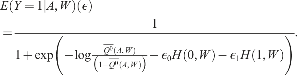
When the initial estimate of
Box 7 – Using the clever covariates and the initial predictions to estimate the fluctuation parameter
An alternative approach, which we will not demonstrate here, is to use clever covariates as weights rather than covariates in this step, which can improve the stability of the estimate. 5
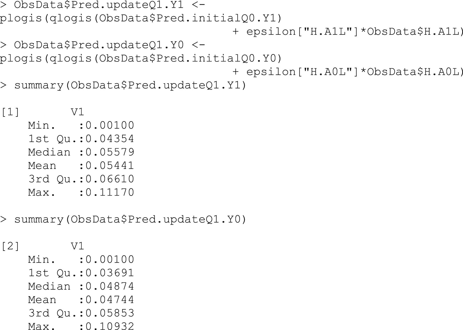
Step 6: Update the initial outcome model prediction based on targeted adjustment of the initial predictions using the PS model
For this step, we define the 
The update to our initial estimate is performed by plugging in the 

Box 8 – Updating predicted counterfactual outcomes using the clever covariates and fluctuation parameter
Step 7: Find treatment effect estimate
The targeted estimate of the ATE is calculated using the following formula, which is an average of the difference between the targeted estimates of the outcomes when treated versus not treated (Box 9)
5
: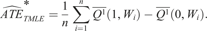
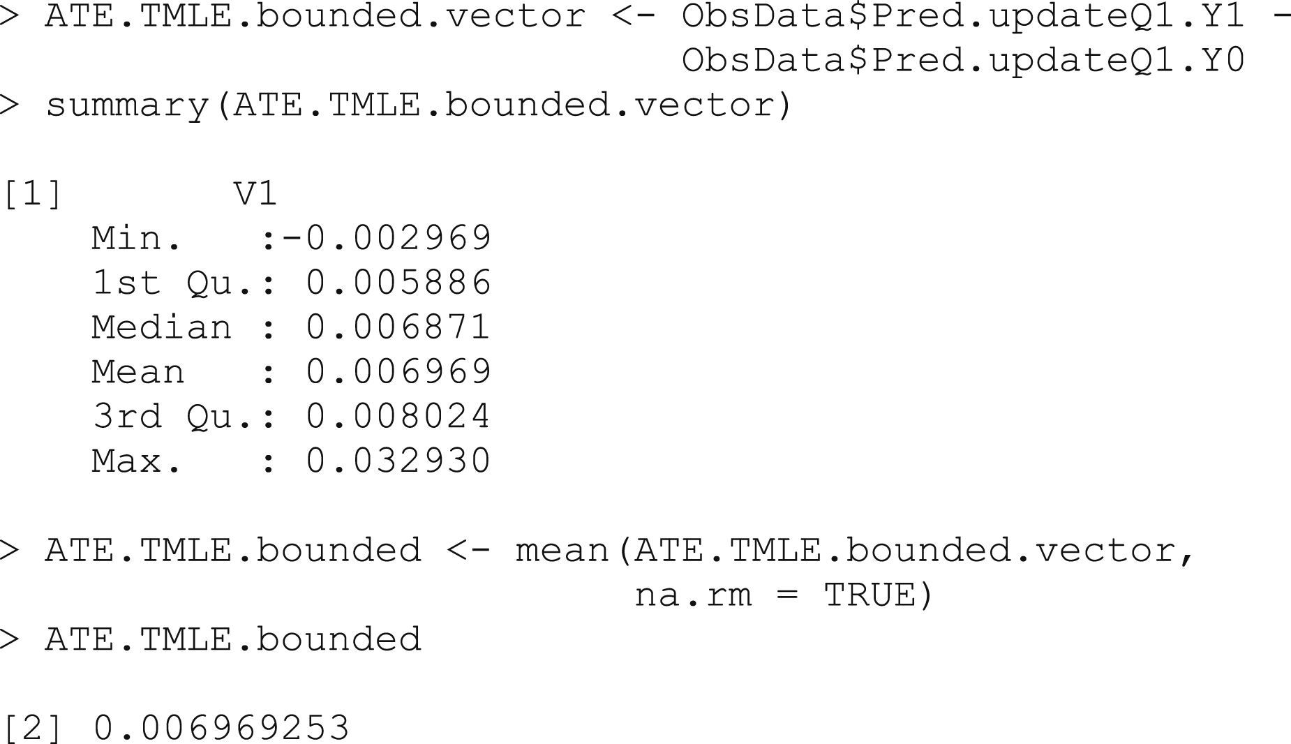
Box 9 – Calculating the ATE by the average difference between updated treated and untreated counterfactual outcomes
Step 8: Transform back the treatment effect estimate to the original outcome scale
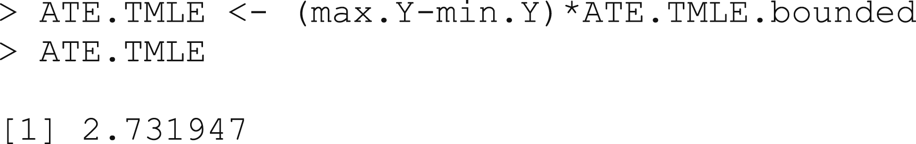
Note that the estimate from the previous step is still on the transformed outcome scale. To interpret our estimate on the original scale, we must use the original bounds of our outcome to transform this estimate back, as shown in Box 10.
3

Box 10 – Transforming the ATE back to the original outcome scale
Step 9: Confidence interval estimation
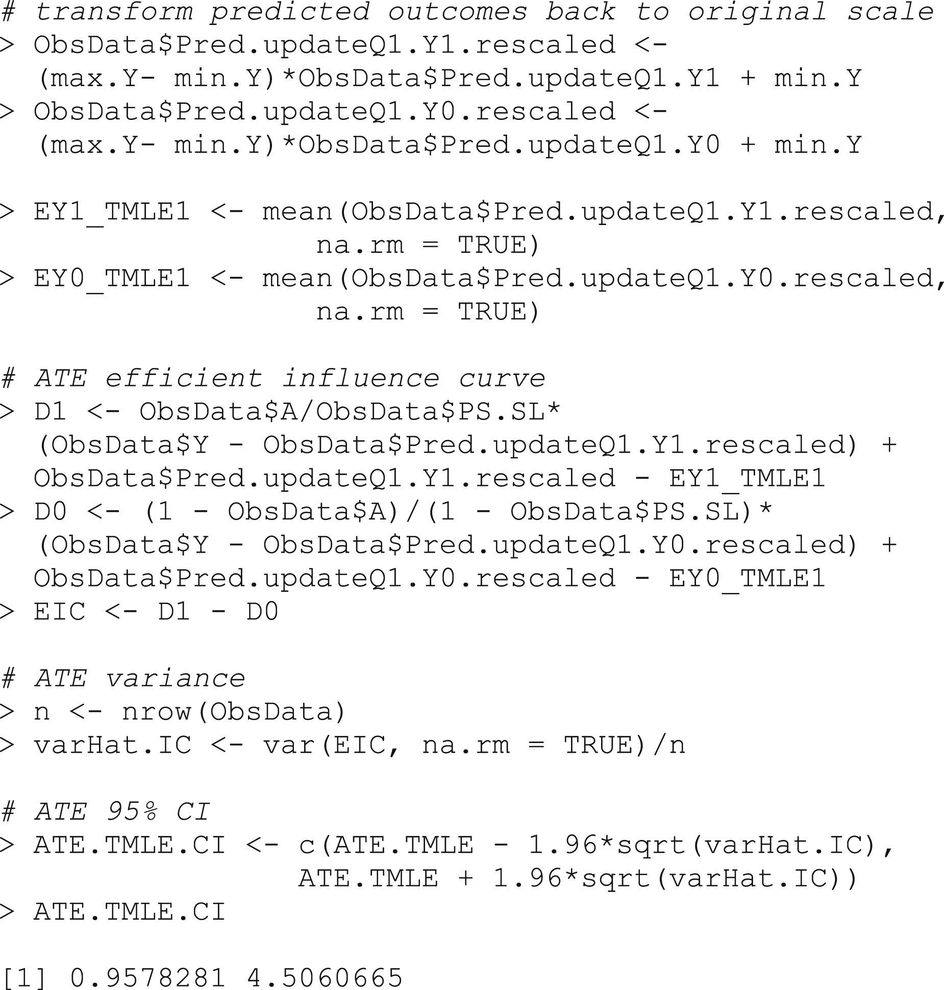
As always, we would like to calculate confidence intervals for our estimated ATE. To do this, we again use the influence function. The influence function has a mean of 0 and a finite variance, which, when divided by the number of observations, corresponds to the variance of the target parameter. There are many influence function options, but there is always an efficient influence function that achieves the lower bound on asymptotic variance (under the modeling assumptions). By finding this efficient influence function and calculating its variance, we can estimate the standard deviation of the parameter and construct confidence intervals for our parameter estimate (Box 11).
5
For the ATE, the efficient influence function is: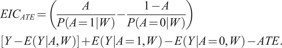
We can estimate this for each subject as: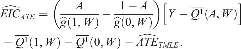
The standard error estimate for our ATE estimate is then: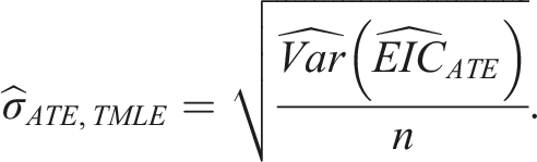
Box 11 – Confidence interval estimation using the efficient influence curve
Pre-packaged TMLE Software
To provide a clear explanation of how TMLE works, we have shown the implementation of each separate step so far. Once the readers understand the implementation details, they can also take advantage of several software packages in R that implement the TMLE steps. 26
tmle
The tmle package can handle both binary and continuous outcomes, and uses SuperLearner to construct the exposure and outcome models just like we did in the steps above (Box 12). Note also that the outcome Y is required to be within the range of
The package’s (version 1.5.0.2) default SuperLearner library for estimating the outcome includes generalized linear models (GLMs), GLM with elastic net regularization, and Bayesian additive regression trees. The default library for estimating the propensity scores also includes GLMs and Bayesian additive regression trees (though specified slightly differently), and replaces the GLM with regularization with generalized additive models (GAMs). 27 More methods can be added by specifying lists of models in the Q.SL.library (for the outcome model) and g.SL.library (for the propensity score model) arguments.
Box 12 – Estimating the ATE using the tmle package
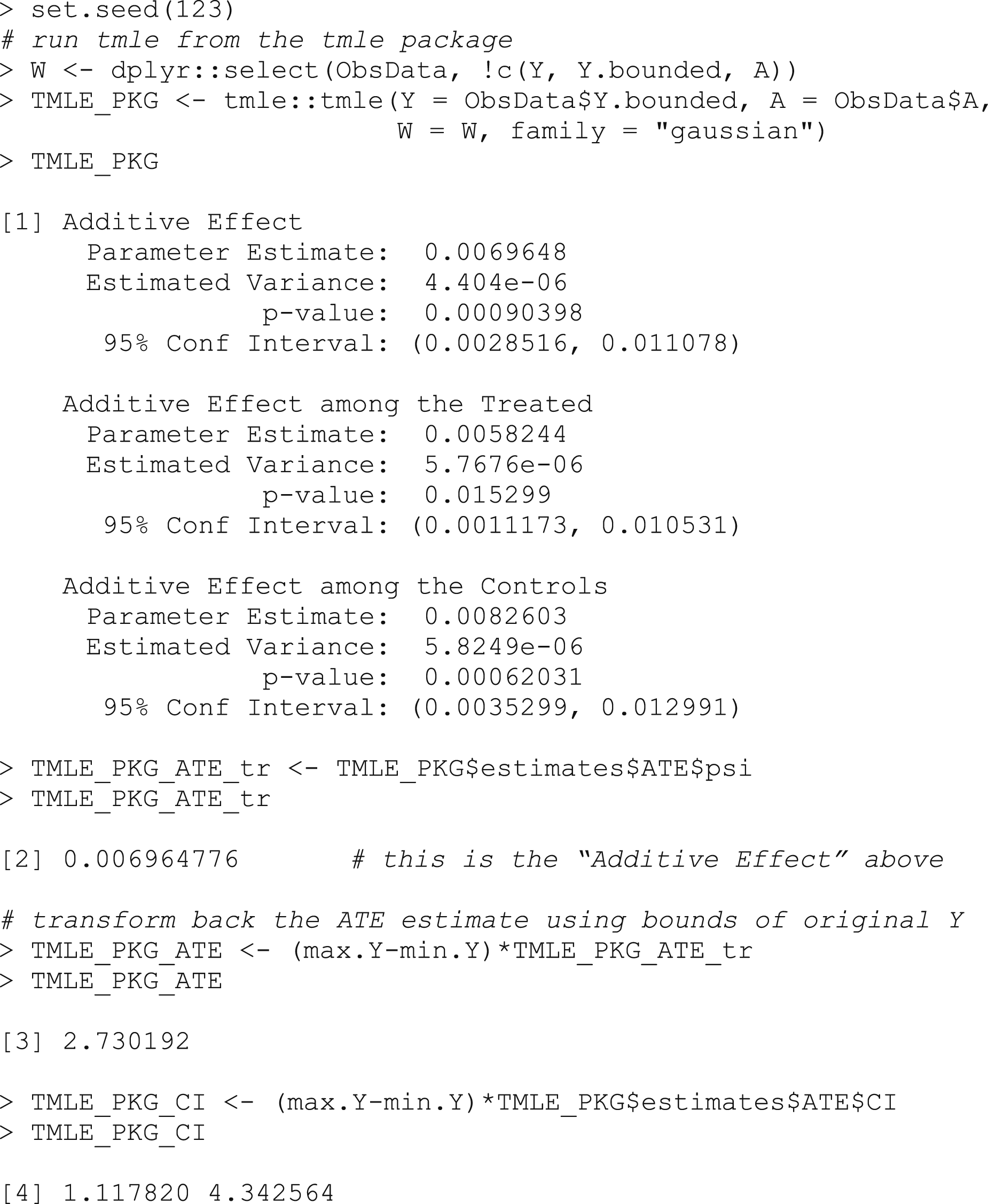
In our first run-through of the step-by-step TMLE process, we used the SuperLearner libraries that the tmle package uses as its default. Our results show a difference in length of stay of 2.73 (0.96, 4.51) days between those who received RHC and those who did not. The point estimate is very similar to the 2.73 (1.12, 4.34) days difference returned by the tmle package. Slight differences could be attributed to the fact that there is some randomness always associated with machine learning algorithms, as you can run the same algorithm multiple times on the same dataset and get slightly different results. Overall, this supports that the steps given in this tutorial are a valid implementation of TMLE and can be referred to for an understanding of how the tmle package works.
Other results reported in literature
Keele paper
Luke Keele and Dylan Small studied a comparison of matching methods and machine learning methods including TMLE in a 2021 study. 28 They reassessed several different datasets, including the RHC dataset with the length of stay outcome. To compare this study’s results with the results of our step-by-step guide, we reran the above steps with the same library of algorithms Keele et al. used in their assessment (Box 13, supplementary materials). The set of algorithms was the same for both the outcome and propensity score models and included generalized linear models (logistic regression), least absolute shrinkage and selection operator (lasso), and random forests. Keele and Small found an average difference in length of stay of 2.01 (0.6, 3.41) days with TMLE with SuperLearner. 28 Our results with the same set of candidate machine learning algorithms showed a difference in length of stay of 2.44 (1.68, 3.20) days. This is not a small difference in results, both in terms of the point estimate and the confidence intervals. Since we did not have sufficient information to replicate the results exactly, it is possible that the difference in results could be attributed to different combinations of variables included in each analysis. The other possibility is that the differences were caused by the random sampling associated with cross-validation in SuperLearner. To minimize the effects of random sampling, we recommend following the flowchart given by Phillips et al. (2022) to select the number of cross-validation folds appropriate for the given sample size. 29
Original connors paper
The original study reported a difference in length of stay of 1.8 days between those treated with an RHC and those not treated with an RHC. This analysis was performed using propensity score matching, a method using the propensity scores calculated in IPTW as a variable to match on rather than as weights on individual observations. 12 The result reported by Connors et al. is not very different from the result reported by Keele and Small, but all TMLE implementations examined resulted in a greater difference than that reported in the initial study, suggesting that the propensity score method’s estimate is probably an underestimate. Another study by Samuels et al. (2018) also used TMLE, among other methods, to reassess this dataset with the length of stay outcome. They report an ATE of 2.73 (1.22, 4.23) for the TMLE method with SuperLearner (implemented using the tmle package, with the default SuperLearner library). 30 This result is again very close to the estimate we got from our TMLE implementation, likely because we used the same library of methods for our SuperLearner that is used by default in the TMLE package. 26 The same study also compared other methods such as bagged one-to-one matching. The estimates using these methods were also higher than the 1.8 days estimated by Connors et al. in the original study. Though we cannot know the true treatment effect, this agreement between TMLE and other methods further supports that the effect reported in the initial study could have been underestimated.
Discussion
In this article, we have described a step-by-step process for implementing TMLE in a continuous outcome setting. This application of TMLE to a well-known real-world dataset should provide practitioners with a transparent understanding of how this method can be used in similar epidemiological settings. Though overall the implementation is similar to the steps used for a binary treatment, it is crucial that we use a transformed outcome and specify a log-likelihood loss function in order to keep the desirable properties TMLE was designed to exhibit. 6 This tutorial complements Luque-Fernandez’s tutorial on TMLE with a binary outcome. 5 Through step-by-step instructions with complete code for an openly accessible dataset, we provide an easy-to-follow and reproducible guide for the application of TMLE in a real-world scenario with a common outcome format. We highlight the benefits of using TMLE with machine learning and validate the results from this guide with those found in literature for the same dataset.
The benefits of using TMLE include the fact that it is doubly robust and thus consistent if either the propensity score model or the outcome model is correctly specified. Additionally, the possibility of using machine learning methods to construct each model decreases the likelihood that the models will be misspecified, while still allowing valid statistical inference with 95% confidence intervals. When using machine learning methods such as SuperLearner in TMLE, it is important to select good parameters for the data in question, including an adequate number of cross-validation folds and a reasonable library of candidate learners. To select appropriate parameters for a certain analysis, we recommend following the guidelines given by Phillips et al. (2022) and Balzer et al. (2021).29,31 TMLE can also be adapted to work with a variety of different outcomes such as longitudinal outcomes, 32 and even different types of treatments such as multiple time point interventions. 33 Recently, TMLE has also been adapted to settings with dependent exposures 34 and time-to-event outcomes, 35 TMLE for use with decision trees and regional exposures, 36 as well as a higher order TMLE that may have improved performance. 37
Augmented inverse propensity weighting (AIPW) is another doubly robust method available. AIPW uses information from the outcome regression model to tweak the inverse probability weighted estimator. 13 The augmentation term based on the outcome model helps to correct the estimate when the treatment mechanism was misspecified. 38 Despite this, TMLE has been shown to provide less biased estimates than AIPW since TMLE is more robust to near positivity violations and TMLE is a plug-in estimator restricting probabilities to be between 0 and 1. 13 Recently, an R package specifically for AIPW estimation was made available. 39
Despite its usefulness, TMLE is not perfect. It still relies on the assumption that there is no unmeasured confounding. Often there are variables we cannot measure or do not even know about, that may influence the exposure and outcome. Unmeasured confounding leads to model misspecification, so TMLE’s assumption that at least one of the outcome and exposure models is correctly specified may not hold. In this case, the TMLE estimator will not be consistent and we may need to use a different method. Additionally, TMLE does not differentiate between instruments and true confounders in the propensity score model, but includes either as long as there is a relationship between the variable and the exposure. 3 This can lead to near or full positivity violations because when we use a SuperLearner to construct the exposure model, it may almost perfectly predict the exposure given a covariate strongly related to the exposure. 40 Improvements could be made by using a double cross-fit procedure with TMLE. This method, by fitting the outcome and treatment models in each split of the data and predicting outcomes using models from discordant splits, addresses non-linearity bias. 41
Future tutorials could focus on different outcome or treatment types, or variations of TMLE. 21 For instance, Collaborative TMLE (CTMLE) is an advancement of TMLE that uses multiple iterations of TMLE to generate an estimate that under certain conditions is consistent even if both models are misspecified. 42 Other extensions could include longitudinal data or multiple time point interventions or other types of data often encountered by practitioners in the real world but complex to analyze.
Footnotes
Declaration of Conflicting Interests
The author(s) declared the following potential conflicts of interest with respect to the research, authorship, and/or publication of this article: MEK is supported by the Michael Smith Foundation for Health Research Scholar award. Over the past 3 years, MEK has received consulting fees from Biogen Inc. for consulting unrelated to this current work.
Funding
The author(s) disclosed receipt of the following financial support for the research, authorship, and/or publication of this article: This work was supported by Dr. Karim’s Natural Sciences and Engineering Research Council of Canada (NSERC) Discovery Grant (PG#: 20R01603) and Discovery Launch Supplement (PG#: 20R12709).
Data Availability Statement
The right heart catheterization dataset used in this tutorial is open source and can be found at https://hbiostat.org/data/ with documentation. The analysis of secondary and de-identified data was exempt from the requirements for research ethics approval both in accordance with the University of British Columbia Policy 89 and in accordance with the provisions of the Tri-Council Policy Statement: Ethical Conduct for Research involving Humans, Article 2.5. The software code used is available in the following GitHub page: ![]() , and additional codes are available in the supplementary materials.
, and additional codes are available in the supplementary materials.