
Abstract
Machine learning (ML) methods for causal inference have gained popularity due to their flexibility to predict the outcome model and the propensity score. In this article, we provide a within-group approach for ML-based causal inference methods in order to robustly estimate average treatment effects in multilevel studies when there is cluster-level unmeasured confounding. We focus on one particular ML-based causal inference method based on the targeted maximum likelihood estimation (TMLE) with an ensemble learner called SuperLearner. Through our simulation studies, we observe that training TMLE within groups of similar clusters helps remove bias from cluster-level unmeasured confounders. Also, using within-group propensity scores estimated from fixed effects logistic regression increases the robustness of the proposed within-group TMLE method. Even if the propensity scores are partially misspecified, the within-group TMLE still produces robust ATE estimates due to double robustness with flexible modeling, unlike parametric-based inverse propensity weighting methods. We demonstrate our proposed methods and conduct sensitivity analyses against the number of groups and individual-level unmeasured confounding to evaluate the effect of taking an eighth-grade algebra course on math achievement in the Early Childhood Longitudinal Study.
Keywords
Over the past decade, there has been a growing interest in using machine learning (ML) methods to estimate the average treatment effect (ATE) and the conditional ATE due to their flexible and near-automatic modeling (Athey & Imbens, 2016; Dorie et al., 2019; Hill, 2011; Imai & Ratkovic, 2013; Künzel et al., 2019; Su et al., 2009; Suk, Kang, et al., 2021; Wager & Athey, 2018). Almost all the ML-based causal inference methods have been designed in a single-level data setting (i.e., independent and identically distributed [i.i.d.] setting) and under the assumption of no unmeasured confounding. But there are limited works on how to utilize ML methods in multilevel data settings to estimate causal effects (Athey & Wager, 2019; Suk & Kang, 2022a, 2022b; Suk, Kang, et al., 2021). The use of ML methods in multilevel data poses new challenges, notably that the data are not i.i.d. and that there is a specific type of unmeasured confounders called cluster-level unmeasured confounders, which may bias causal estimates. The overall goal of this article is to design ML-based causal inference methods that are insensitive to cluster-level unmeasured confounding while maintaining ML methods’ strengths on flexible and near-automatic modeling. In this article, we focus on multisite/multilevel observational data, where the treatment is assigned at the unit level (e.g., students), not at the cluster level (e.g., schools).
Cluster-level confounders are covariates that (1) are shared by individuals within a cluster and (2) affect both the treatment and the outcome of interest. When cluster-level confounders are present and not adjusted for, they distort the treatment effect by making a spurious association between the treatment and outcome (Arpino & Mealli, 2011; Li et al., 2013). For example, consider the kindergarten cohort of the Early Childhood Longitudinal Study (ECLS-K) and suppose we are interested in studying the causal effect of students taking an eighth-grade algebra course on their math achievement. Algebra courses are mathematics courses offered in U.S. school systems, and prior studies have advocated policies that encourage students to take algebra prior to entering high school (Rickles, 2013). These studies also found that school-level characteristics such as school location, school composition, and school processes play a key role in students’ mathematics course-taking and their performance on achievement tests (Anderson & Chang, 2011; Cogan et al., 2001; Opdenakker & Van Damme, 2001). Unfortunately, the ECLS-K data did not measure all possible school-level confounders, such as school’s funding for math education and school principal’s emphasis on STEM education, and estimating the treatment effect consistently becomes a challenge.
When we suspect cluster-level unmeasured confounders in multilevel studies, it is important to eliminate or alleviate their impact on the effect estimates. Suk and Kang (2022a, 2022b) have started to explore how to make ML methods more robust to cluster-level unmeasured confounding. Their strategies include using a new loss function that is insensitive to cluster-level unmeasured confounding, injecting propensity scores estimated from fixed effects logistic regression or random effects logistic regression, and employing cluster dummy variables or cluster-demeaned variables. But all these strategies seek to train ML methods by using the entire sample from all the clusters rather than using only a subsample within each cluster or within each group of similar clusters. That is, previous works are based on an across-cluster approach rather than a within-cluster approach or a within-group approach, where groups are constructed by combining similar clusters.
Different grouping approaches in multilevel data have been frequently compared in particular for propensity score methods (Arpino & Cannas, 2016; Arpino & Mealli, 2011; Kim & Seltzer, 2007; Lee et al., 2021; Leite et al., 2015; Li et al., 2013; Rickles & Seltzer, 2014; Schuler et al., 2016; Thoemmes & West, 2011). Briefly, an across-cluster approach uses the entire sample to estimate a propensity score model across clusters; a within-cluster approach uses the subsample within each cluster to estimate a cluster-specific propensity score model (Kim & Seltzer, 2007; Leite et al., 2015; Thoemmes & West, 2011); a within-group approach uses the subsample within each group to estimate a group-specific propensity score model, where groups consist of multiple clusters (Kim & Steiner, 2015; Lee et al., 2021; Suk & Kim, 2019). Among different approaches, a within-cluster approach is the most flexible and the most robust to bias from cluster-level unmeasured confounders, but it becomes unstable when cluster sizes are small (Kim & Seltzer, 2007; Thoemmes & West, 2011). In contrast, under small cluster sizes, a within-group approach performs better than a within-cluster approach by combining similar clusters into groups, and it is more flexible and more robust to cluster-level unmeasured confounding than an across-cluster approach (Lee et al., 2021). Although there are advantages and disadvantages of different grouping approaches for the propensity score, unfortunately, there is little research on examining comprehensive options to using ML methods for causal inference in multilevel studies.
The main goal of this article is to investigate a within-group approach to using ML methods for robustly estimating the ATE in multilevel studies when cluster-level unmeasured confounders are present. In this article, clusters (e.g., schools) represent sites where study units (e.g., students) belong, and groups refer to a collection of clusters. We focus on one particular ML-based causal inference method based on the targeted maximum likelihood estimation (TMLE) with an ensemble learning algorithm (Luque-Fernandez et al., 2018; van der Laan & Rose, 2011), but we believe our main ideas can be easily applied to other ML methods. At a high level, our proposal constructs groups of similar clusters based on treatment prevalence and uses “vanilla” TMLE or model-assisted TMLE to estimate the treatment effects within each group. Specifically, vanilla TMLE consists of implementing the default TMLE as is, that is, using the propensity score and the outcome predictions from the default ensemble learning algorithms. Model-assisted TMLE consists of injecting multilevel propensity scores estimated from fixed effects or random effects logistic regression models that can account for cluster-level unmeasured confounding. A major strength of our proposal is that it makes an existing TMLE estimator robust to cluster-level unmeasured confounding. Additionally, unlike parametric propensity score methods, our ML-based proposal has the potential to increase robustness under model misspecification. In short, our proposal simultaneously enjoys robustness from model misspecification and cluster-level unmeasured confounding. Also, to the best of our knowledge, this article is the first attempt to use different options other than an across-cluster approach to design robust ML methods in multilevel studies, with one possible exception of Suk, Kim, et al. (2021). Suk, Kim, et al. (2021) classified clusters into latent classes based on latent class regression models to estimate latent heterogeneity of treatment effects, but their method is not robust to bias from unmeasured confounders.
For evaluating the performance of our proposed methods, we conduct simulation studies that vary multiple parameters such as the number of groups, the working model of the propensity score, and whether there is a cross-level interaction between a cluster-level unmeasured confounder and a treatment variable. We also compare our proposed methods to existing parametric-based methods, especially propensity score weighting methods. Lastly, we demonstrate the proposed methods in our example above about evaluating the ATE of taking an eighth-grade algebra course on math achievement, and we conduct sensitivity analyses about the number of groups and individual-level unmeasured confounding where the latter is based on a recent proposal by Chernozhukov et al. (2021).
Notations, Estimand, and Assumptions
To formalize causal effects, we use the potential outcomes notation (Neyman, 1923; Rubin, 1974). Suppose that we have j = 1, 2, …, J clusters, where each cluster has 1, 2,…, nj
individuals. We denote Zij
∈ {0, 1} as a binary treatment variable, where Zij
= 1 represents that individual i in cluster j received the treatment and Zij
= 0 represents that individual i in cluster j did not receive the treatment. We denote Yij
(1) as the potential treatment outcome if individual ij were treated (Zij
= 1), we denote Yij
(0) as the potential control outcome if individual ij were untreated (Zij
= 0), and we denote Yij
as individual ij’s observed outcome. Finally, we denote
The target estimand of interest in this article is the ATE. Under the potential outcomes framework, it is defined as the average linear contrast between the potential treatment outcome and the potential control outcome:
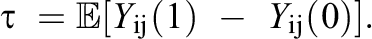
For instance, in our empirical ECLS-K data, the ATE measures the overall average effect of students taking an eighth-grade algebra course on math achievement. The typical set of working assumptions to identify the ATE from observational data (Hernan & Robins, 2020; Imbens & Rubin, 2015; Rubin, 1986) is (A1) Stable Unit Treatment Value Assumption (SUTVA)
(A2) Conditional Ignorability: (A3) Positivity: 0 < eij < 1 where
where Assumptions (A2) and (A3) are jointly referred to as strong ignorability (Rosenbaum & Rubin, 1983). In words, Assumption (A1) means that individual ij’s potential outcomes are independent of others’ treatment assignments and there is only one version of the treatment. Assumption (A2) means that the treatment status Zij
is conditionally independent of the potential outcomes Yij
(1) and Yij
(0) given all the confounders

The above identification strategy requires all the confounders to be available in the observed data. However, even if
Existing Estimation Methods for Handling Cluster-Level Unmeasured Confounding in Multilevel Observational Studies
In this section, we review popular estimators of the ATE in the presence of cluster-level unmeasured confounding. We first summarize propensity score weighting methods among various types of propensity score methods, notably matching, stratification, and weighting (Arpino & Mealli, 2011; Kim & Seltzer, 2007; Leite et al., 2015; Li et al., 2013; Rickles & Seltzer, 2014; Schuler et al., 2016; Thoemmes & West, 2011). 1 We then review recent approaches, one by Lee et al. (2021) based on using treatment prevalence to remove cluster-level unmeasured confounding and another by Suk and Kang (2022a, 2022b) based on designing robust ML methods under cluster-level unmeasured confounding.
Propensity Score Weighting Estimators
Broadly speaking, propensity score weighting estimators consist of two main steps: first, estimating a propensity score and, second, using the estimated propensity score as sampling weights to estimate the ATE. For estimating the propensity score in multilevel observational studies, investigators typically use either a within-cluster propensity score model or an across-cluster propensity score model; a within-cluster propensity score model estimates the propensity score within each cluster, and an across-cluster propensity score model uses a single propensity score model with fixed effects or random effects for all the clusters (Arpino & Mealli, 2011; Leite et al., 2015; Li et al., 2013; Schuler et al., 2016). Within-cluster propensity score models are the most flexible but may not be appropriate when (1) treatment selection processes are extremely strong (e.g., retention, disability diagnosis), (2) cluster sizes are small, or (3) there are clusters with only treated units or only control units (Kim & Seltzer, 2007; Leite et al., 2015; Thoemmes & West, 2011). Across-cluster propensity score models with cluster-specific fixed effects or random effects remedy these concerns from within-cluster propensity score models but make additional assumptions about the propensity score model. See Arpino and Mealli (2011), Li et al. (2013), and Schuler et al. (2016) for more information on propensity score models with random effects or fixed effects.
The next step is to estimate the ATE using the estimated propensity scores above, and one of the most popular estimators is by inverse propensity weighting (IPW). Specifically, an IPW estimator uses propensity scores as a form of sampling weights in order to achieve covariate balance between the treatment group and the control group. There are two main types of IPW estimators: the marginal IPW estimator and the clustered IPW estimator. A marginal IPW estimator, denoted as τ^MIPW, produces a weighted difference in the mean overall outcome between treated units and control units and is formalized as follows (Li et al., 2013):
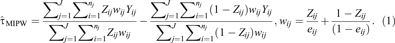
In contrast, a clustered IPW estimator, denoted as τ^CIPW, produces a weighted average of cluster-specific ATE estimates (Li et al., 2013):
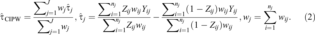
The main difference between the marginal IPW estimator and the clustered IPW estimator is that the clustered IPW estimator with a correctly specified propensity score model guarantees within-cluster covariate balance, whereas the marginal IPW estimator does not. But the clustered IPW estimator requires each cluster to have at least one treatment unit and one control unit, whereas the marginal IPW estimator does not require such a condition. We provide formulas for standard errors of IPW-based estimators in Supplemental Appendix A.
Within-Group Propensity Score Weighting Estimator
Recently, Lee et al. (2021) proposed a new approach to estimate the ATE in the presence of cluster-level unmeasured confounders by grouping clusters with similar proportions of treated individuals, that is, treatment prevalence. Specifically, for each cluster j = 1,…, J, let
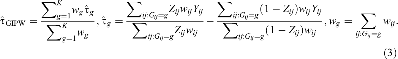
Intuitively, this grouping strategy reduces bias arising from a cluster-level unmeasured confounder Uj because the observed treatment prevalence is affected by both observed and unobserved covariates; in other words, it contains information about the unobserved confounder Uj . Grouping clusters with similar treatment prevalence likely leads to grouping clusters with similar values of Uj if the selection models are homogeneous across clusters (or groups of clusters); see He (2018, p. 13) for a formal result under some modeling assumptions. Also, Lee et al. (2021) reveal that among the aforementioned IPW estimators, the grouped IPW estimator is more robust to cluster-level unmeasured confounding than the marginal IPW estimator and the grouped IPW estimator also performs better than the clustered IPW estimator in particular when cluster sizes are small. Lastly, Lee et al. (2021) numerically examined the impact of using four different approaches to grouping: (1) random grouping, (2) grouping based on treatment prevalence, (3) grouping based on measured covariates only, and (4) grouping based on treatment prevalence and measured covariates. Through a simulation study, they found that grouping clusters with similar treatment prevalence produces the smallest average bias of the ATE. See Lee et al. (2021) for details, notably a theoretical justification of the grouped IPW estimator and simulation results about different choices of grouping.
Robust ML Methods Under Cluster-Level Unmeasured Confounding
Recently, Suk and Kang (2022a, 2022b) studied how to design robust ML methods under cluster-level unmeasured confounding. Briefly, Suk and Kang (2022a) provide three ML-based estimators to estimate the ATE and the conditional ATE in the presence of cluster-level unmeasured confounders. The three proposed estimators—the proxy regression estimator, the double demeaning estimator, and the double demeaning estimator with proxy regression—require writing a new loss function that is insensitive to cluster-level unmeasured confounders and solving for the minimum of the loss function. Also, they are designed based on an ensemble supervised learning algorithm like SuperLearner (van der Laan et al., 2007). While these proposed estimators hold promise for eliminating the impact of cluster-level unmeasured confounding, their proposal cannot be directly applied to retune or refit the existing ML methods to enhance ML’s robustness.
In contrast, Suk and Kang (2022b) studied five modifications of causal forests (Athey et al., 2019; Wager & Athey, 2018) to make it robust to cluster-level unmeasured confounding. For brevity, their proposed modifications consist of injecting propensity scores estimated from random effects or fixed effects logistic regression, adding cluster dummy variables, and using cluster-demeaned variables (without or with including cluster-demeaned propensity scores). Notably, they found that the modifications based on using multilevel propensity scores estimated from fixed effects logistic regression or using cluster-demeaned variables along with demeaned propensity scores display the most promise for eliminating bias from cluster-level unmeasured confounders.
While these prior works provide effective tools to robustify ML methods for causal inference, all their proposals are designed based only on an across-cluster approach, which uses the entire sample from all the clusters to estimate the propensity score (or the outcome model) across clusters. Examining different options to designing robust ML methods rather than an across-cluster approach has not been explored yet.
Our Proposal: Within-Group TMLE
In this section, we focus on one popular ML-based causal inference method, TMLE generally combined with an ensemble of supervised learning algorithms. We present a brief summary of TMLE and ensemble learning. We then present our proposed modifications to TMLE to be robust to cluster-level unmeasured confounding.
Vanilla TMLE
We briefly review the TMLE estimator. TMLE is a general framework for constructing efficient and double-robust substitution estimators and is commonly implemented with an ensemble learning algorithm (Balzer et al., 2019; Luque-Fernandez et al., 2018; van der Laan & Rose, 2011). The estimator first requires an initial estimator of the outcome regression, denoted as
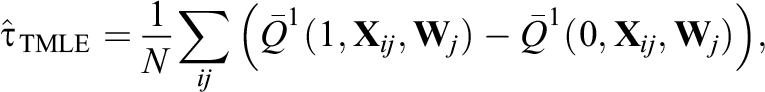
where N represents the total sample size, that is,
Importantly, TMLE can incorporate ML methods to estimate
Our Modifications for TMLE
We propose three modifications to make TMLE robust to cluster-level unmeasured confounding. The proposed modifications require constructing groups of similar clusters based on treatment prevalence and using vanilla TMLE or model-assisted TMLE to estimate the treatment effects within each group. Vanilla TMLE comprises implementing the default TMLE as is, and model-assisted TMLE comprises injecting multilevel propensity scores estimated from fixed effects or random effects logistic regression models (see Table 1 for a summary).
Summary of Modifications in Targeted Maximum Likelihood Estimation (TMLE)
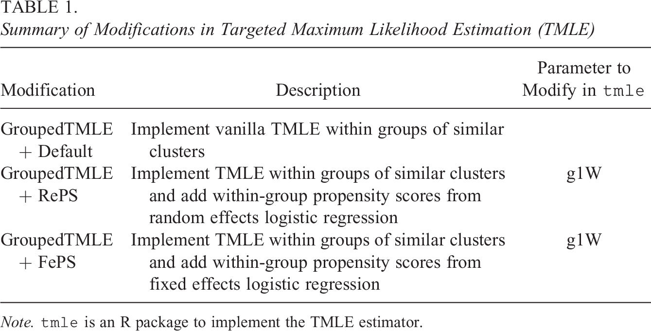
Note.
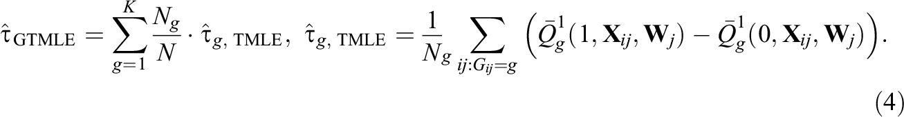
Our first proposed modification, denoted as GroupedTMLE, is to form groups of similar clusters based on treatment prevalence and then implement TMLE within each group g (g = 1, 2,…, K). To create groups of clusters, we use K-means clustering (Hartigan & Wong, 1979; MacQueen et al., 1967), one of the most popular grouping/clustering methods in education and psychology. Briefly, K-means clustering is an iterative algorithm that categorizes the data into K distinct nonoverlapping groups. Its goal is to make the intragroup observations as similar as possible, and it does this by minimizing the following total group variance (Hastie et al., 2009):
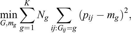
where pij
indicates individual ij’s treatment prevalence; mg
indicates the mean of group g (g = 1,…, K); Ng
indicates the sample size in group g. In our setting, because our group assignment variable is cluster-specific (i.e., pij
= pi’j
= pj
), individuals in the same cluster will belong to the same group. Also, for each group g = 1,…, K, we let
Our second modification, denoted as GroupedTMLE+RePS, is an extension of the first modification using the within-group approach but additionally forces TMLE to use random effects propensity scores within each group; this can be implemented by using the parameter g1W in the tmle package. Specifically, we fit the following within-group, random effects propensity score models as

In Equation 5, the cluster-specific main effect

In Equation 6, the term
The second and third modifications are motivated from (i) the study by Suk and Kang (2022b) and (ii) the doubly robust property of the TMLE estimator. Among five modifications by Suk and Kang (2022b), we use modifications using random effects propensity scores and fixed effects propensity scores because they are easy to implement. If we correctly specify fixed effects or random effects propensity score models within each group and inject them inside TMLE, it becomes robust to bias from cluster-level unmeasured confounders and will yield a consistent estimator of the ATE. Also, as we can see from the simulations in the following, even if we use partially misspecified propensity scores inside TMLE within each group, the proposed within-group TMLE still produces robust ATE estimates compared to their IPW counterparts due to the double robustness and the flexible modeling of the outcome regression Q.
We make some remarks about the proposed modifications. First, when the number of groups is equal to one, it is equivalent to an across-cluster approach where all the clusters are used at once to fit the propensity score model or the outcome model. To reduce confusion in this article, when the number of groups is larger than or equal to 2, we call the approach the within-group approach. Second, other existing grouping/clustering methods can be used to classify J clusters into K groups based on each cluster’s treatment prevalence such as partitioning around medoids (Kaufman & Rousseeuw, 2009) or finite mixture models (Clogg, 1995; McLachlan & Peel, 2000). Third, the elbow method, the gap statistics method (Tibshirani et al., 2001), and/or the covariate balance check within each group would be used for choosing the number of groups in our context; see Supplemental Appendix B for an illustration of the elbow method with our simulation designs.
Simulation Study
We conducted simulation studies to assess the performance of our purposed, within-group TMLE methods and to compare our proposal with non-ML, IPW methods. Table 2 summarizes the methods for estimating propensity scores and the ATE in simulation studies. As for propensity scores, we use both across-cluster propensity scores (K = 1) and within-group propensity scores (K ≥ 2), and we estimate propensity scores with different estimation models: random effects models, fixed effects models, and if applicable, default ensemble learning algorithms. Also, we use four different ATE estimators: the marginal IPW estimator in Equation 1, the clustered IPW estimator in Equation 2, the grouped IPW estimator in Equation 3, and the grouped TMLE estimator in Equation 4.
Summary of Methods for Estimating Propensity Scores (PS) and the Average Treatment Effect (ATE) in Simulation Studies
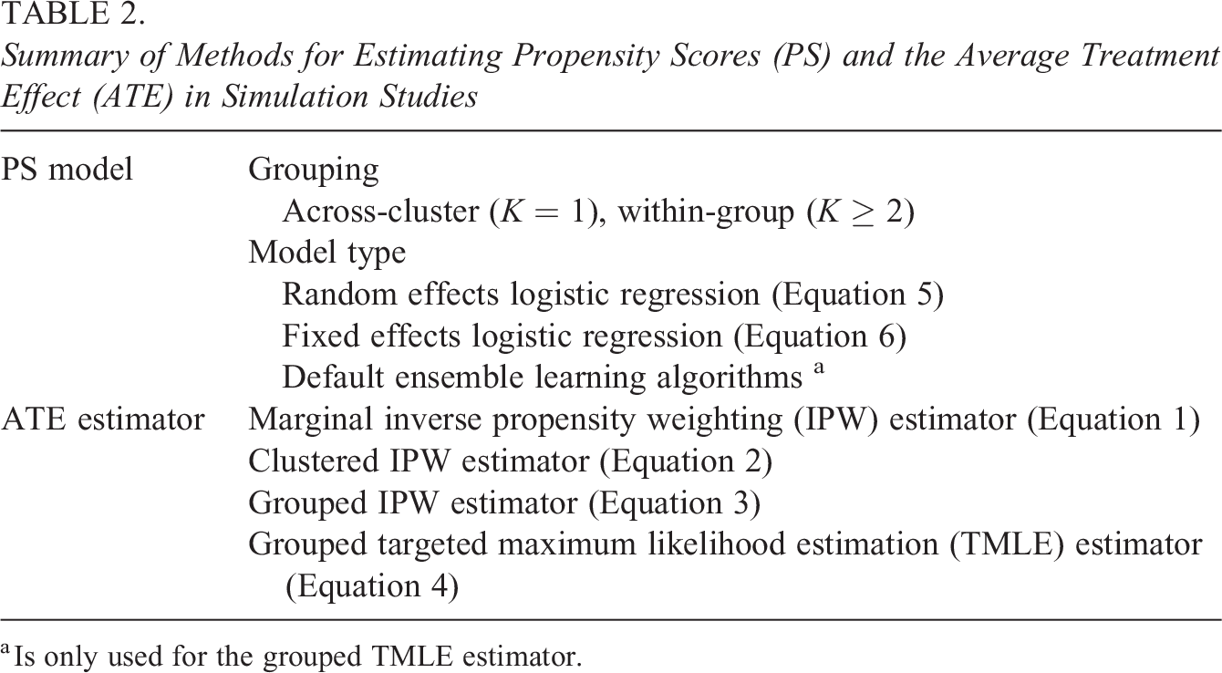
a Is only used for the grouped TMLE estimator.
Specifically, our simulation studies are categorized into three designs. Design 1 assumes no cross-level interaction between a cluster-level unmeasured confounder and the treatment variable (i.e., β 1 = 0 below). Design 2 assumes that there exists a cross-level interaction between the two (i.e., β 1 = 2 below). Design 3 is based on Design 2 but uses a misspecified propensity score model by excluding one threshold term. In particular, Design 3 considers a more realistic scenario, in which a meticulous researcher, despite their efforts, was successful in correctly specifying some parts of the propensity score model. For each design, we used 15 different group numbers ranging from 1 to 15, and using only one group is equivalent to using an across-cluster, ungrouped approach. As mentioned above, to reduce confusion, when the number of groups is larger than or equal to 2, the approach is referred to as a within-group approach.
For all the designs, we examined the performance of the proposed methods in each design by repeating the simulation 500 times, and we evaluated the performance of each estimator by measuring the absolute bias (|Bias|), standard deviation (SD), and root mean squared error (RMSE) defined as follows:
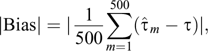
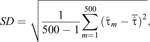
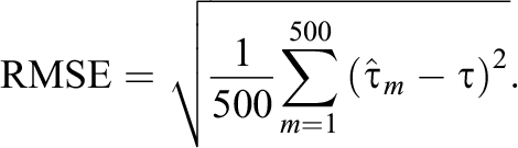
Here,
Design 1: No Cross-Level Interaction
The data generating models are stated in the following and are based on those from Lee et al. (2021), Li et al. (2013), Suk and Kang (2022b), and our empirical data. 1. For each cluster j = 1, 2, … , 170, generate the total number of individuals in each cluster nj
by drawing a number from a normal distribution with mean 15 and small SD and rounding it to the nearest integer. We remark that this sample size condition is comparable to that of our empirical ECLS-K data. 2. For each individual i = 1, … , nj
in cluster j, generate individual-level confounders,


Note that we also use the data generating models, where all the covariates have the same scale and follow the same distribution: Uniform (−1, 1). The simulation results are provided in Supplemental Appendix F, and the result patterns generally agree with those from the above data generating models.
3. Generate individual treatment status Zij from the logistic propensity score model as follows:

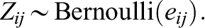
The propensity score model contains a nonlinear, threshold term (i.e., I(X 2ij < 0.3)).
4. Generate the potential outcomes Yij (1), Yij (0), and observed outcome Yij from the regression model as follows:
Here, rij is the random error for individual i in cluster j. The term β 1 is a cross-level interaction effect between Uj 3 and the treatment variable. The population ATE, τ, is E(2 + 2X 3ij + 2Wj + β 1 Uj 3 ) = 3. In this design, we used β 1 = 0 to reflect the absence of the cross-level interaction between the cluster-level unmeasured confounder and the treatment variable.
Comparison of different estimators
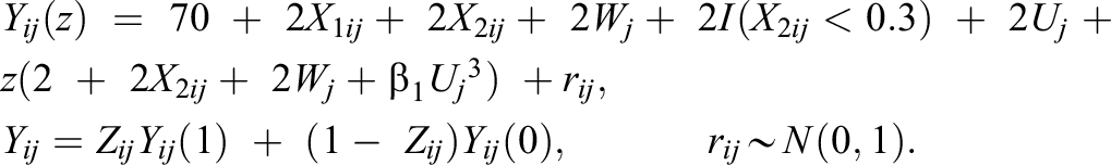
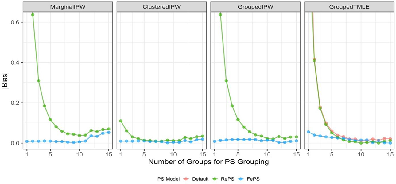
Figure 1 summarizes the absolute bias of the ATE estimates across different numbers of groups in propensity score models, where each panel shows the absolute bias from one of the four ATE estimators investigated; see numerical results in Supplemental Appendix C. Also, parametric-based IPW estimators use either within-group propensity scores from random effects logistic regression (denoted as RePS) or within-group propensity scores from fixed effects logistic regression (denoted as FePS). The ML-based TMLE estimator uses RePS, FePS, and within-group propensity scores from the default ensemble learning algorithm (denoted as Default).
Performance of average treatment effect estimates in Design 1. Propensity scores (PS) used in estimators are within-group propensity scores from random effects logistic regression (RePS), within-group propensity scores from fixed effects logistic regression (FePS), or if applicable, within-group propensity scores from default ensemble learning algorithms (Default). MarginalIPW = the marginal inverse propensity weighting estimator; ClusteredIPW = the clustered inverse propensity weighting estimator; GroupedIPW = the grouped inverse propensity weighting estimator; GroupedTMLE = the grouped targeted maximum likelihood estimation estimator.
Among non-ML methods, we observe that the marginal IPW estimator with within-group, fixed effects propensity scores (MarginalIPW+FePS) produces little bias and performs better than the marginal IPW estimator with within-group, random effects propensity scores (MarginalIPW+RePS). But as the number of groups increases, MarginalIPW+RePS’s performance greatly improves and is similar to that of MarginalIPW+FePS. We also observe that the absolute bias from the marginal IPW estimators is somewhat increased as the number of groups increases from 10 to 15. This may be because students coming from K ≥ 10 different groups but with the identical propensity scores may have different covariates and using them together inside the marginal IPW estimator might not yield covariate balance, either in the entire sample or within each cluster.
In contrast, the performance of the clustered IPW estimators (ClusteredIPW+RePS and ClusteredIPW+FePS) is insensitive to propensity score estimation methods and the number of groups, and the clustered estimators yield little bias. This is expected given that the clustered IPW estimators aggregate cluster-specific ATE estimates that are robust to cluster-level unmeasured confounding. Regarding the grouped IPW estimators, the grouped estimators with two different types of propensity scores (GroupedIPW+RePS and GroupedIPW+FePS) perform no worse than the corresponding marginal estimators (MarginalIPW+RePS and MarginalIPW+FePS). In particular, the grouped IPW estimators produce almost zero bias in the ATE estimates when we use more than 10 groups, compared to the marginal IPW estimators. This implies that when using within-group propensity scores, it is desirable to estimate the ATE by aggregating group-specific ATEs, not directly estimating the ATE across clusters.
Among ML methods, the grouped TMLE estimator with default ensemble learning algorithms (GroupedTMLE+Default) shows improved performance as the number of groups increases. This obviously implies that using the within-group approach makes the TMLE estimator more robust to cluster-level unmeasured confounding. When we use the grouped TMLE with our additional modifications using either random effects propensity scores or fixed effects propensity scores (GroupedTMLE+RePS and GroupedTMLE+FePS), we also observe that similar to non-ML methods, GroupedTMLE+FePS performs better than GroupedTMLE+RePS, but both modified TMLE estimators show enhanced performance compared to that using default ensemble learning algorithms, that is, GroupedTMLE+Default. Moreover, additional benefits from using multilevel propensity scores inside TMLE are larger when the number of groups K is small, and in particular, using TMLE with fixed effects propensity scores under K = 1 shows the largest bias reduction compared to TMLE with default ensemble learning algorithms. When we use a larger number of groups, there are minor or subtle benefits from injecting fixed effects propensity scores or random effects propensity scores. These results indicate that using the proposed within-group approach is a primary contributing factor that minimizes bias in ATE estimates from cluster-level unmeasured confounding and using the additional modification with fixed effects propensity scores on top of that is a safer way to eliminate the bias. We remark that we observe similar performance patterns in terms of RMSE; see Supplemental Appendix C for details.
Comparison of different grouping options
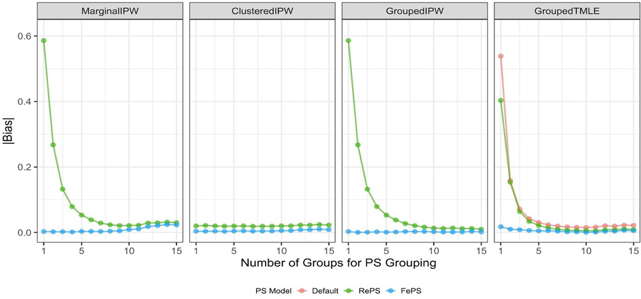
In this section, we used different grouping options, where we changed our inputs inside K-means clustering for within-group TMLE methods. We used grouping based on treatment prevalence as our baseline, and we considered three additional options: (1) random grouping, (2) grouping based on measured cluster-level covariates, and (3) grouping based on treatment prevalence and measured cluster-level covariates. Here, measured cluster-level covariates contain not only measured covariates naturally shared among individuals (i.e.,
Performance of average treatment effect estimates from the grouped targeted maximum likelihood estimation estimator in Design 1 with different grouping options. Propensity scores (PS) used in the estimator are within-group propensity scores from random effects logistic regression (RePS), within-group propensity scores from fixed effects logistic regression (FePS), and within-group propensity scores from default ensemble learning algorithms (Default).
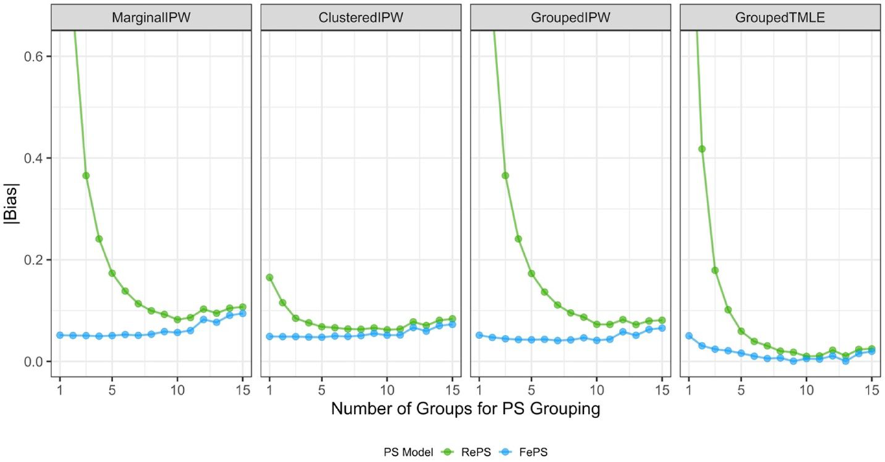
Design 2: Cross-Level Interaction
Design 2 used the same data generating models as Design 1 except that we used β 1 = 2, where we assume the presence of a cross-level interaction between the cluster-level unmeasured confounder and the treatment variable. We summarize the absolute bias of the ATE estimates in Figure 3. To have the same range as Figure 1, Figure 3 only shows the absolute bias ranging from 0 to 0.62 and Supplemental Appendix D contains the numerical results. As expected, the absolute bias is amplified in general compared to Design 1, and yet, we observe the common patterns of the estimators investigated between the two designs. Similar to Design 1, the performance of the estimators using fixed effects propensity scores is better than that of the corresponding estimators using random effects propensity scores. When the number of groups K is relatively larger (say, more than 10), the marginal IPW estimators yield increasing bias in the ATE estimates, similar to Design 1. In contrast, the other three estimators—clustered IPW, grouped IPW, and grouped TMLE—produce more robust estimates by forming multiple groups of similar clusters and using within-group propensity scores. In particular, a monotonic decrease in bias from the grouped TMLE estimators is observed with an increase in the number of groups. But unlike Design 1, the clustered IPW estimators (ClusteredIPW+RePS and ClusteredIPW+FePS) no longer have flat patterns and we see relative performance differences across propensity score methods and/or the number of groups; we observe relatively larger bias from ClusteredIPW+RePS when the ATE estimates are aggregated by using propensity scores with K = 1 or K = 2. This indicates that in the presence of the cross-level interaction, the clustered estimator with random effects propensity scores is no longer robust when coupled with the propensity score model that is ungrouped (K = 1) or grouped with a few numbers of groups (e.g., K = 2). This observation is partly because the clustered estimator itself is not robust to bias from cross-level interaction. It may also result from the fact that impact of using random effects models that are inherently misspecified under our data generating models (Uj ∼ Uniform(−2, 2)) is the largest with K = 1 or K = 2.
Design 3: Cross-Level Interaction and Partially Misspecified Propensity Score Models
In this design, we used the same design as Design 2, but we omitted a threshold term when fitting a multilevel propensity score model with either random effects or fixed effects. As mentioned above, we included partially misspecified multilevel propensity scores inside our modified TMLE. This design considers a realistic situation, in which a meticulous researcher, despite their best efforts, may not be able to specify the perfectly correct propensity score model. Figure 4 summarizes the absolute bias of the ATE estimates. Similar to Figure 3, Figure 4 only shows the absolute bias ranging from 0 to 0.62, and Supplemental Appendix E includes the numerical results. As predicted, all the non-ML methods—the marginal IPW, the clustered IPW, and the grouped IPW estimators—yield more biased estimates than those from the corresponding estimators in Design 2; the resulting ATE estimates have nonnegligible bias arising from using partially misspecified propensity scores, regardless of the number of groups formed.
Performance of average treatment effect estimates in Design 2. Propensity scores (PS) used in estimators are within-group propensity scores from random effects logistic regression (RePS), within-group propensity scores from fixed effects logistic regression (FePS), or if applicable, within-group propensity scores from default ensemble learning algorithms (Default). All conditions for which absolute bias exceeded 0.62 were omitted to compare the performance with that from Design 1. MarginalIPW = the marginal inverse propensity weighting estimator; ClusteredIPW = the clustered inverse propensity weighting estimator; GroupedIPW = the grouped inverse propensity weighting estimator; GroupedTMLE = the grouped targeted maximum likelihood estimation estimator.
Performance of average treatment effect estimates in Design 3. Propensity scores (PS) used in estimators are within-group propensity scores from random effects logistic regression (RePS), within-group propensity scores from fixed effects logistic regression (FePS). All conditions for which absolute bias exceeded 0.62 were omitted to compare the performance with that from Design 1. MarginalIPW = the marginal inverse propensity weighting estimator; ClusteredIPW = the clustered inverse propensity weighting estimator; GroupedIPW = the grouped inverse propensity weighting estimator; GroupedTMLE = the grouped targeted maximum likelihood estimation estimator.
In contrast, injecting partially misspecified propensity scores into our ML-based methods, the grouped TMLE estimators, is unlikely to seriously weaken their effectiveness with respect to the absolute bias, compared to the performance of the corresponding grouped TMLE estimators in Design 2. Most importantly, the grouped TMLE estimators are much more robust than all non-ML methods with the same degree of misspecification. That is, TMLE’s flexible modeling and double robustness potentially alleviate the impact of misspecifying propensity scores in TMLE. We remark that the overall patterns of RMSE lines are similar to those of the bias lines, though we see more fluctuation with respect to RMSE; see Supplemental Appendix E for details.
Overall, across different simulation designs, the proposed within-group TMLE method with fixed effects propensity scores is effective in reducing bias from cluster-level unmeasured confounders and this bias reduction is most pronounced when there are eight or more groups. We summarize takeaways from the simulation results in the following: Based on the performance of GroupedTMLE+Default, creating groups of clusters based on treatment prevalence shows great promise in training TMLE to produce more robust estimates to cluster-level unmeasured confounding. Adding fixed effects propensity scores to the grouped TMLE estimator (i.e., GroupedTMLE+FePS) performs better than adding random effects propensity scores (i.e., GroupedTMLE+RePS). The bias reduction from injecting multilevel propensity scores is larger when only a few numbers of groups are constructed. With more than six groups, the additional benefit declines. Even if multilevel propensity scores are partially misspecified, training TMLE with them may potentially alleviate bias from cluster-level unmeasured confounding, in particular compared to non-ML IPW estimators with the same degree of misspecification.
Real Data Study
Data and Variables
We demonstrate our proposed within-group ML methods by studying the effects of taking an eighth-grade algebra course with the ECLS-K data. ECLS-K is a national longitudinal study to investigate the school achievement and student experiences from kindergarten to middle school. It is sponsored by the National Center for Education Statistics. ECLS-K collected a nationally representative sample of kindergarteners in the fall of 1998 from a dual-frame multistage sampling design and followed them from the fall of 1998 to the spring of 2007 when most were in eighth grade (Walston & McCarroll, 2010). For more information about the ECLS-K study and data, see the ECLS-K website: http://nces.ed.gov/ecls/kindergarten.asp. Following the data analysis procedure used in Suk and Kang (2022b), we used both the fifth-grade assessment data in the spring of 2004 and the eighth-grade assessment data in the spring of 2007. The 2004 data were used to obtain pretreatment covariates (e.g., prior achievement scores, gender) that affect the treatment mechanism and the outcome process based on prior works about algebra courses in middle school (Rickles, 2013; Rickles & Seltzer, 2014; Suk & Kang, 2022b; Walston & McCarroll, 2010). We used the 2007 data to obtain the treatment and outcome variables.
Our data analysis used a binary treatment variable, a continuous outcome variable, and 11 pretreatment covariates. Specifically, the treatment variable represents whether a student took an eighth-grade algebra course in the spring of 2007, and it was binary where 1 denotes that they took an algebra or higher level course and 0 denotes that they took a lower level math course. The outcome variable was students’ math achievement scores in the spring of 2007. We assume that math achievement scores for eighth graders in the spring of 2007 are a posttreatment variable for the following two reasons; first, ECLS-K data collection in the spring of 2007 was conducted at least two months after the beginning of the Spring semester (Tourangeau et al., 2009), and second, the eighth grade algebra course is usually a yearlong course, beginning in the Fall semester. As for pretreatment covariates, eight of these 11 covariates were at the student level and contain prior math achievement scores, parents’ expectation of their child’s highest level of education, gender, race, socioeconomic status, poverty level, mother’s educational level, and family type (i.e., living with one parent or two parents). The rest of the covariates were at the school level and contain school type (i.e., public vs. private), school location (i.e., urban, suburb, small town), and region (i.e., West, Northeast, South, Midwest). We made the outcome and all continuous covariates standardized with a mean of 0 and an SD of 1. In total, the analytic sample consisted of 2,581 students from 170 schools with a mean school size of 15.8. The mean and the SD of the unstandardized, observed math scores are 145.78 and 19.67, respectively.
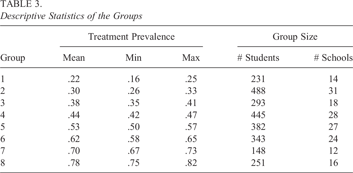
We ran the proposed within-group TMLE methods to estimate the ATE of students taking an eighth algebra course on math achievement. As a comparison, we used the marginal IPW, clustered IPW, and grouped IPW estimators, all with within-group propensity scores. The eight groups (i.e., K = 8) were chosen because of the simulation results above and nonviolation of the positivity assumption. Table 3 provides the descriptive statistics of the eight groups. The smallest group mean of the treatment prevalence is 0.22, whereas the largest group mean is 0.78. Each group has at least 10 schools (i.e., clusters) and more than 140 students (i.e., units).
Descriptive Statistics of the Groups
Finally, we conducted sensitivity analyses with respect to the number of groups and individual-level unmeasured confounding. First, we checked the sensitivity of our conclusions by changing the number of groups, in particular to K = 1 and K = 7. We chose K = 1 because it would lead to the largest difference if the cluster-level unmeasured confounders were present, and we chose K = 7 because it is the second largest number that satisfies the positivity assumption. Second, we conducted a sensitivity analysis to assess whether our conclusions about the ATE would be altered when an individual-level unmeasured confounder is assumed to be present. For the sensitivity analysis, we used a nonparametric approach based on partial R 2 (Pearson’s correlation ratio) from Chernozhukov et al. (2021), where the bounds on the size of the bias are determined by the residualized outcome, residualized treatment, and plausible partial R 2 of the unobserved confounder with the outcome and the treatment. Using the estimated standard errors (or confidence intervals) of the original estimates, we report the confidence intervals of the adjusted estimates in the presence of such an individual-level unmeasured confounder.
Regarding software, we used the built-in R function kmeans for grouping the treatment prevalence, the tmle package (Gruber & van der Laan, 2012) for the TMLE estimator, and the lme4 package (Bates et al., 2015) for random effects logistic regression. Data and R codes are available in Supplementary Materials and the first author’s GitHub repository (https://github.com/youmisuk/groupedTMLE).
Results
Table 4 provides the ATE estimates of taking an eighth-grade algebra course using the proposed within-group TMLE methods as well as non-ML-based IPW methods. The unadjusted mean difference in math scores between students who took algebra and those who did not, often referred to as the prima facie effect, is 0.676 (not shown in Table 4). After applying different estimators with within-group propensity scores, the adjusted estimates are smaller than the unadjusted estimate, but most of them are still significantly positive. See Supplemental Appendix G for covariate balance, and we achieved acceptable covariate balance between the treatment group and control group under each type of propensity scores.
Average Treatment Effect (ATE) Estimates of Taking an Eighth-Grade Algebra Course on Math Achievement
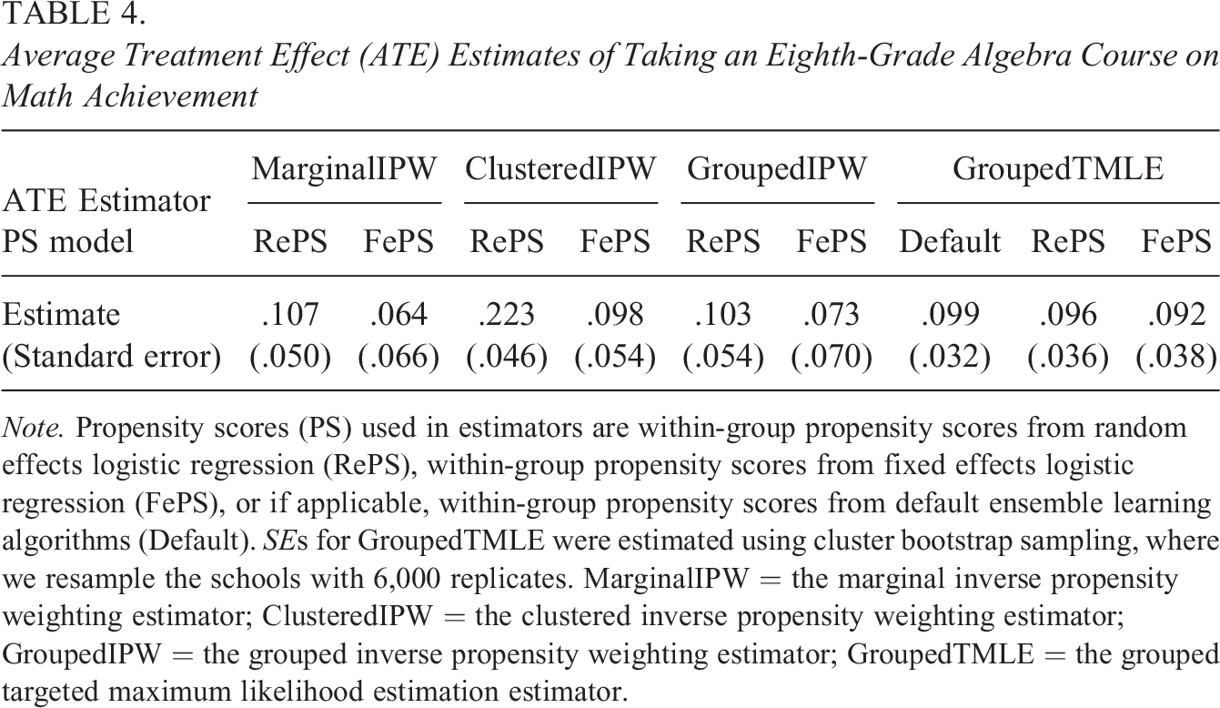
Note. Propensity scores (PS) used in estimators are within-group propensity scores from random effects logistic regression (RePS), within-group propensity scores from fixed effects logistic regression (FePS), or if applicable, within-group propensity scores from default ensemble learning algorithms (Default). SEs for GroupedTMLE were estimated using cluster bootstrap sampling, where we resample the schools with 6,000 replicates. MarginalIPW = the marginal inverse propensity weighting estimator; ClusteredIPW = the clustered inverse propensity weighting estimator; GroupedIPW = the grouped inverse propensity weighting estimator; GroupedTMLE = the grouped targeted maximum likelihood estimation estimator.
Among non-ML methods (i.e., MarginalIPW, ClusteredIPW, and GroupedIPW), we observe that ATE estimates based on within-group, random effects propensity scores were larger than the corresponding estimates based on within-group, fixed effects propensity scores. The grouped IPW estimator produced similar estimates to those from the marginal estimator in the ECLS-K data. As shown in simulations above, ATE estimates from non-ML IPW estimators may not be reliable if the propensity score model is misspecified. In contrast, the ML-based TMLE estimator (i.e., GroupedTMLE) potentially produces more robust ATE estimates when we suspect model misspecification, and we see that there were very small variations in ATE estimates from the proposed grouped TMLE estimator across different types of propensity scores. Regarding standard errors, the estimates from fixed effects propensity scores have slightly larger standard errors than those from random effects propensity scores. This is expected because the fixed effects models yield larger variability mainly due to the small cluster size. Based on our simulation results and “Our Modifications for TMLE” section, we assume that ATE estimates from the grouped TMLE estimator with within-group propensity scores are more reliable, robust estimates to bias from cluster-level unmeasured confounding and model misspecification. Overall, we conclude that there is a positive effect of taking an eighth-grade algebra course on students’ math achievement scores.
Next, we conducted a sensitivity analysis regarding different numbers of groups when we used the most extreme Ks (here, K = 1 and K = 7), and we provide the results in Table 5. Under ungrouped propensity scores (i.e., K = 1), all the ATE estimates were slightly larger than the respective estimates in Table 4, though the differences are not large enough to be statistically significant. Note that under K = 1, the marginal IPW and grouped IPW estimators produce identical results. When we formed seven groups (K = 7), the estimates from IPW-based estimators with random effects propensity scores and grouped TMLE estimators were very similar to those in Table 4. The estimates from IPW-based estimators with fixed effects propensity scores were somewhat different from those in Table 4, and these differences may be due to the remaining imbalance in the covariates with fixed effects propensity scores under K = 7; see Supplemental Appendix H for details. Overall, our conclusions about the ATE have not been altered by forming seven groups.
Results of the Sensitivity Analysis Regarding the Number of Groups
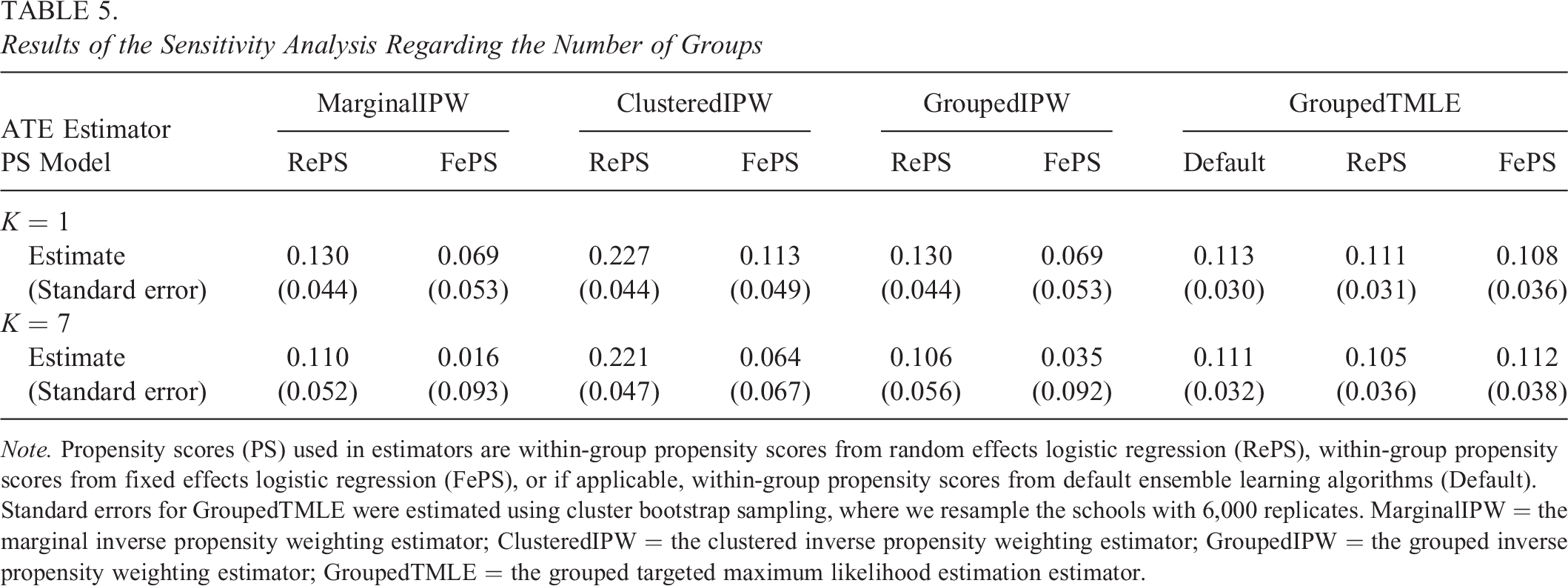
Note. Propensity scores (PS) used in estimators are within-group propensity scores from random effects logistic regression (RePS), within-group propensity scores from fixed effects logistic regression (FePS), or if applicable, within-group propensity scores from default ensemble learning algorithms (Default). Standard errors for GroupedTMLE were estimated using cluster bootstrap sampling, where we resample the schools with 6,000 replicates. MarginalIPW = the marginal inverse propensity weighting estimator; ClusteredIPW = the clustered inverse propensity weighting estimator; GroupedIPW = the grouped inverse propensity weighting estimator; GroupedTMLE = the grouped targeted maximum likelihood estimation estimator.
Finally, we examined whether our conclusions about the ATE would be changed by biases from the individual-level unmeasured confounder Uij
. For the sensitivity analysis, we focus on ATE estimates from within-group TMLE methods that produce more robust ATE estimates from cluster-level unmeasured confounding and model misspecification. Following Chernozhukov et al. (2021), we determined bounds on the target parameter
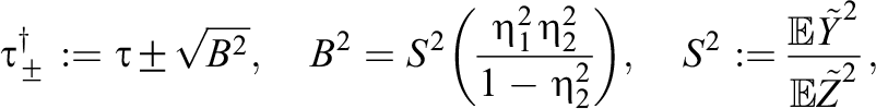
where
Using the above sensitivity analysis, our adjusted 95% confidence intervals for the ATE with the positive bias (i.e., +B) are: [0.165, 0.290] for GroupedTMLE+Default, [0.124, 0.265] for GroupedTMLE+RePS, and [0.128, 0.274] for GroupedTMLE+FePS. 3 All the confidence intervals did not contain 0, and thus, we did not alter our conclusions about the effect estimates. We also computed the adjusted 95% confidence intervals with the negative bias (i.e., −B), and they are: [0.014, 0.138] for GroupedTMLE+Default [−0.024, 0.118] for GroupedTMLE+RePS, and [−0.024, 0.123] for GroupedTMLE+FePS. Confidence intervals with TMLE using multilevel propensity scores contained 0, and thus, we would alter our conclusions about the effect estimates if the negative bias were present. From the results of the sensitivity analysis, we conclude that the ATE estimates from the grouped TMLE estimator with multilevel propensity scores would not be robust if an individual-level unmeasured confounder exhibited negative bias.
Conclusions
The goal of this article was to provide a within-group approach to enhance the performance of ensemble ML methods for causal inference, particularly, TMLE, in multilevel observational data under cluster-level unmeasured confounding. We proposed three different modifications for TMLE, so that it can be more robust to cluster-level unmeasured confounding, and we compared the performance of each modified TMLE method with that of the marginal IPW estimator, the clustered IPW estimator, and the grouped IPW estimator. Through our simulation studies, we find evidence to support the effectiveness of our proposal. Training vanilla TMLE based on a within-group approach (i.e., GroupedTMLE+Default) makes TMLE robust to cluster-level unmeasured confounding, and in particular, when the number of groups is more than or equal to 8, most of the bias is eliminated. Using model-assisted TMLE using within group, multilevel propensity scores also helps remove bias, and the modification using fixed effects logistic regression (i.e., GroupedTMLE+FePS) has the best potential for reducing bias from cluster-level unmeasured confounders. Additionally, unlike parametric propensity score methods, our ML-based proposal has the potential to increase robustness under model misspecification. Lastly, we demonstrated the use of our proposed ML methods on the ECLS-K data, and we find that there is a positive effect of taking an eighth-grade algebra course on math achievement scores and our ATE estimates from within-group TMLE methods with multilevel propensity scores may be sensitive to individual-level unmeasured confounding.
There are some limitations of this article. First, we did not explore how to determine the appropriate number of groups for the within-group TMLE method. Researchers can use methods such as the Elbow method or gap statistics method, as well as examining within-group covariate balance to determine the optimal number of groups. While we recommend using eight or more groups based on our setting, the ideal number of groups will depend on various design factors such as the number of clusters and the impact of unmeasured cluster-level confounders on the outcome model. As this article primarily focuses on introducing within-group ML methods, further investigation into this issue will be explored in future research. Second, our additional modifications were based on using a simple input tuning parameter inside TMLE (i.e., g1W), and we did not utilize other tuning parameters that may affect the performance of TMLE in clustered settings, such as a different set of ensemble learning algorithms and the use of an optional subject identifier. Third, we did not consider comprehensive simulation parameters that characterize multilevel observational data, such as the sample size and different clustering structure. We only used a fixed total sample size of about 2,550 (170 clusters with a mean cluster size of 15) in the simulations, which was comparable to the sample size of our ECLS-K data. We also did not examine more complex cluster structure beyond two level data, such as three-level data and cross-classified data. Fourth, we assumed SUTVA in multilevel data, where the treatment is hypothesized to not have spillover/peer effects through interference within clusters.
Despite these limitations, we believe that our modifications of within-group TMLE can enhance the performance of original TMLE in multilevel observational studies faced with cluster-level unmeasured confounding and our main ideas can be easily applied to other ML-based casual inference methods. Although no amount of statistical methodology can remove all the omitted variable bias, we believe developing robust methods helps practitioners narrow down the sources of the omitted variable bias and have a more focused set of questions about evaluating whether their effect estimates are plausibly causal or not. We hope that the findings of this article can serve as useful guidelines for researchers who like to fine-tune ML-based causal inference methods or apply the robust machinery to multilevel observational data in order to assess causal effects of programs or policies in education and the social sciences.
Supplemental Material
Supplemental Material, sj-pdf-1-jeb-10.3102_10769986231162096 - A Within-Group Approach to Ensemble Machine Learning Methods for Causal Inference in Multilevel Studies
Supplemental Material, sj-pdf-1-jeb-10.3102_10769986231162096 for A Within-Group Approach to Ensemble Machine Learning Methods for Causal Inference in Multilevel Studies by Youmi Suk in Journal of Educational and Behavioral Statistics
Footnotes
Declaration of Conflicting Interests
The author(s) declared no potential conflicts of interest with respect to the research, authorship, and/or publication of this article.
Funding
The author(s) disclosed receipt of the following financial support for the research and/or authorship of this article: This research was supported by a grant from the American Educational Research Association which receives funds for its “AERA Grants Program” from the National Science Foundation under NSF award NSF-DRL #1749275. The opinions reflected here are those of the author and do not necessarily reflect those of AERA or NSF.
Notes
References
Supplementary Material
Please find the following supplemental material available below.
For Open Access articles published under a Creative Commons License, all supplemental material carries the same license as the article it is associated with.
For non-Open Access articles published, all supplemental material carries a non-exclusive license, and permission requests for re-use of supplemental material or any part of supplemental material shall be sent directly to the copyright owner as specified in the copyright notice associated with the article.