Sage Journals: Discover world-class research

Abstract

A mining complex or mineral value chain is an integrated system composed of mines, stockpiles, waste disposal and tailings facilities, processing destinations and transportation, that leads to generating sellable products delivered to customers and/or the spot market. To deal with such a system, conventional approaches optimise the related components independently and sequentially, while ignoring the related uncertainties. This article extends the simultaneous stochastic optimisation of mining complexes, so as to incorporate equipment uncertainties in addition to supply uncertainty. The inclusion of multiple components and different sources of uncertainty empowers the optimisation to capitalise on the synergies between the different components of a mining complex, while also managing the related technical risk and maximising the net present value. An application at a copper mining complex demonstrates the applied aspects of the proposed approach that jointly considers supply and equipment uncertainty to generate life-of-asset production schedules with a 2% higher net present value, when compared to the results considering only supply uncertainty.

Keywords

Mining complex simultaneous stochastic optimisation stochastic mine planning equipment uncertainty geological uncertainty mine production scheduling

Introduction

A mining complex can be considered as an integrated mineral value chain that transforms in-situ raw material extracted from mineral deposits into valuable commodities, with components including multiple mineral deposits, stockpiles, processing streams, waste disposal and transportation to clients or spot markets (Goodfellow and Dimitrakopoulos, 2016, 2017; Montiel and Dimitrakopoulos, 2015, 2017; Pimentel et al., 2010). Over the past decade, significant developments have been achieved in integrating various components within the mineral value chain into a single optimisation model while considering uncertainty. This integrated model for mining complexes enables the simultaneous optimisation of diverse decisions, such as the extraction sequence, destination policies and processing stream utilisation, and incorporates uncertainties presented in mining complexes. The simultaneous stochastic optimisation leverages the value of the final products sold and captures synergies across the value chain, facilitating comprehensive and efficient decision-making for mining operations.

Conventionally, the components of a mining complex are optimised separately and sequentially (Hustrulid et al., 2013). In the past, several developments have advanced the conventional approach toward joint optimisation by incorporating multiple components of a mining complex in the planning process. Hoerger et al. (1999a, 1999b) presented a mixed integer programming (MIP) formulation to capture the synergies of jointly optimising the flow of material tonnage between mines, stockpiles, and processing plants by maximising the net present value; however, in this case, mine production schedules are a pre-determined input. The Blasor mine planning software of BHP (Stone et al., 2007) simultaneously optimises the proportion of material extracted from multiple pits for long-term mine planning using a MIP model. However, it aggregates spatially connected blocks to reduce the number of integer variables, such that the size of the MIP is reduced and can be solved in a reasonable time. Whittle and Whittle (2007) proposed an approach that includes multiple mines, stockpiles and processing destinations in a mining complex to capture synergies. However, it employs several optimisation procedures throughout the mineral value chain rather than in a single formulation. Each mine is optimised separately first to produce a sequence of pushbacks within its optimised pit limit. Then, interactions between components, modelled by the processing and blending strategies, are optimised to improve the outcome of the mining complex using heuristics approaches (Whittle, 2018). The above-mentioned approaches have limitations, which include aggregate blocks to reduce the computational complexities and the use of estimated (average type) orebody models of the deposit. The latter ignores the uncertainty and spatial variability of pertinent properties of the mineral deposit, which is a major source of technical risk in mine planning, referred to as supply or geological uncertainty (Dowd, 1994, 1997; Ravenscroft, 1992), and affects the grades and material types of the deposit. It misrepresents the impacts on the economic value of the mine production schedule; therefore, the integration of supply uncertainty with stochastic simulations into optimisation algorithms is required to enhance the robustness of the mining complex optimisation and its ability to capture synergies (Dimitrakopoulos et al., 2002).

In response to the above limitations, the simultaneous stochastic optimisation of mining complexes incorporates all of the components of a mining complex into a single mathematical formulation, while also accounting for uncertainties (Goodfellow and Dimitrakopoulos, 2016; Montiel and Dimitrakopoulos, 2015). Montiel and Dimitrakopoulos (2015) presented a simultaneous stochastic optimisation model that can incorporate multiple mineral deposits, multiple processing streams and multiple transportation alternatives. The block extraction sequence and processing destination, as well as the processing and transportation alternatives, are optimised simultaneously in the presence of supply uncertainty. Montiel and Dimitrakopoulos (2018) introduced an extension that integrates specific operational constraints for creating practical mine production schedules. The study includes a large-scale application and comparisons with conventional methods at the Twin Creeks gold mining complex in Nevada. Montiel and Dimitrakopoulos (2017) introduced a metaheuristic algorithm designed to solve the extensive optimisation model of mining complexes. The case study conducted at a copper deposit showed that, compared to a mine plan generated by conventional mine planning software, the simultaneous stochastic optimisation model was able to reduce deviations in capacity from 9% to 0.2%, while increasing the expected net present value by 30%. Goodfellow and Dimitrakopoulos (2016) presented a generalised network-based modelling method that allows for the inclusion of every component in a mining complex for the simultaneous stochastic optimisation and considers the value of the final products sold at the end of the mining complex, instead of block economic values. The method aims to define simultaneously the life-of-asset extraction sequence, destination policy and processing stream decisions while managing the production targets. The model can be easily adapted for any mining complex. In the given case study, the simultaneous stochastic optimisation of mining complexes manages the technical risk associated with geological uncertainty. A case study (Goodfellow and Dimitrakopoulos, 2017) is performed on a copper-gold mining complex, in comparison to the conventional schedule and resulted in an increase of the net present value (NPV) by 22.6%, while also more closely meeting production targets and managing the associated geological risk. Due to its generalised and adaptable formulation, subsequent research has tested the framework introduced by Goodfellow and Dimitrakopoulos (2016) through a large variety of applications incorporating various aspects of mining operations. Farmer (2017) expands the generalised model to incorporate capital expenditure (CapEx) and mining capacity decisions, incorporating these aspects into an application with intricate revenue streams, including streaming agreements. Del Castillo and Dimitrakopoulos (2019) expanded the mathematical formulation to include a dynamic optimisation for strategic planning explicitly including CapEx alternatives and different operating modes. Accounting for the flexibility of an operation, the multi-stage model is able to react and adapt to new information over the life of a mining complex by allowing the solutions to branch. Kumar and Dimitrakopoulos (2019) presented an application incorporating geo-metallurgical decisions into the destination policy at a large copper–gold mining complex. Saliba and Dimitrakopoulos (2019) presented another application that accounts for both supply uncertainty and market uncertainty through commodity price simulations at a gold mining complex. In summary, simultaneous stochastic optimisation offers several advantages, including capturing synergies among different components, managing risk associated with material supply uncertainty, avoiding misrepresentation of mining selectivity by aggregating mine blocks into large volumes, and focusing on the value of the product sold rather than the value of the mining blocks. The documented benefits of simultaneous stochastic optimisation include increased metal quantity, higher NPV, reliable production forecasts, integrated waste production and quality management, as well as the joint integration of supply and demand uncertainty (Dimitrakopoulos and Lamghari, 2022).

The developments discussed above assume constant equipment capacities, such as fixed truck and shovel capacity. However, the impact of uncertain equipment performance on long-term mine production scheduling in simultaneous stochastic optimisation remains unexplored. Recent simultaneous stochastic optimisation applications that address equipment uncertainty primarily concentrate on short-term optimisation for specific sections of the mine, defined by the long-term plan. The related stochastic optimisation approaches for short-term planning and their applications aim, given the long-term plan, to minimise operational costs by optimising shovel and truck activities, as well as uncertainties related to equipment that are often modelled by making prior assumptions about the distribution models (Both and Dimitrakopoulos, 2020; Matamoros and Dimitrakopoulos, 2016; Paduraru and Dimitrakopoulos, 2018; Quigley and Dimitrakopoulos, 2020). For example, Both and Dimitrakopoulos (2020) used distribution with known means and standard deviations for generating equiprobable stochastic simulations of shovel productivity for modelling equipment uncertainty. The research highlights the benefits of simultaneously optimising the mining complex with equipment decisions, leading to cost savings from optimised equipment movements and enhanced equipment utilisation. However, the short-term production plan is constructed on shorter timescales and designed to meet the targets of the long-term production plan, which does not consider equipment uncertainty, and thus needs to be explored.

In the following sections, an extension of the simultaneous stochastic optimisation method proposed by Goodfellow and Dimitrakopoulos (2016) to incorporate uncertain equipment performance in the long-term production planning of mining complexes is presented. Then, the quantification of equipment uncertainty is outlined. Subsequently, a case study of the copper mining complex is presented to incorporate both supply and equipment uncertainty and explore the potential improvements from incorporating equipment uncertainty into the optimisation process. Last, conclusions and future work are presented.

Method

Notation

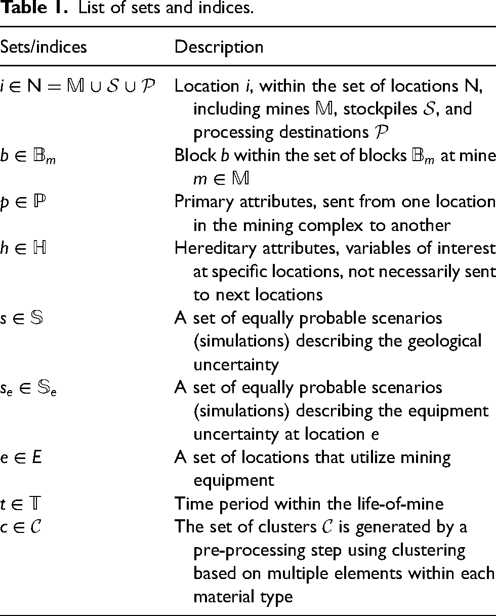
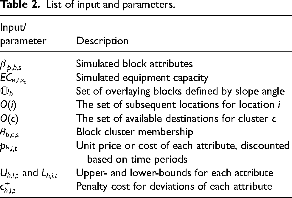
An example of a mining complex or mineral value chain is shown in Figure 1. Sets and indices used for the mathematical formulation of the simultaneous stochastic optimisation of mining complexes are presented in Table 1. Inputs and parameters are listed in Table 2.

Figure 1.

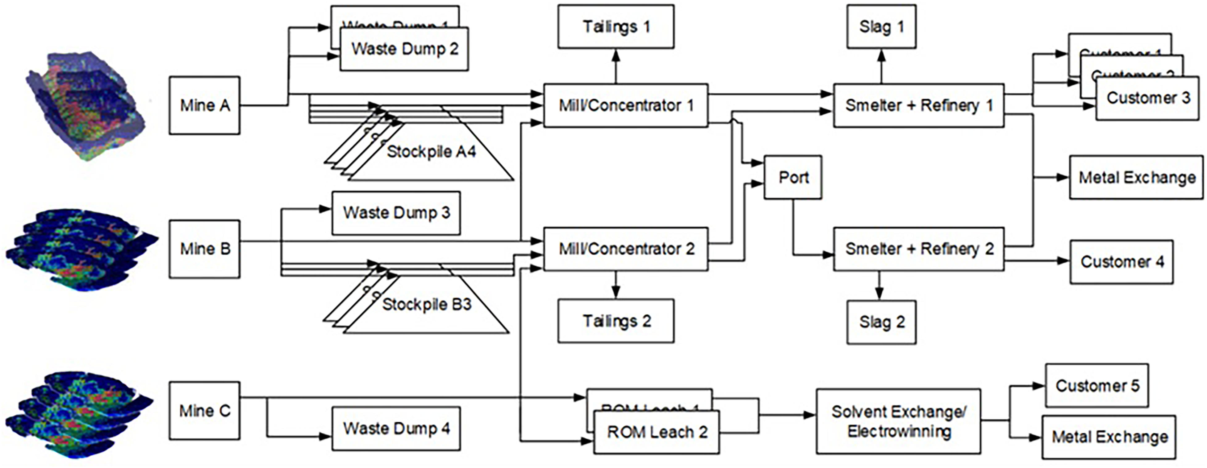
An example of a mining complex.

Table 1.

List of sets and indices.

Sets/indices	Description
$i \in N = M \cup S \cup P$	Location i, within the set of locations $N$ , including mines $M$ , stockpiles $S$ , and processing destinations $P$
$b \in B_{m}$	Block b within the set of blocks $B_{m}$ at mine m ∈ $M$
$p \in P$	Primary attributes, sent from one location in the mining complex to another
$h \in H$	Hereditary attributes, variables of interest at specific locations, not necessarily sent to next locations
$s \in S$	A set of equally probable scenarios (simulations) describing the geological uncertainty
$s_{e} \in S_{e}$	A set of equally probable scenarios (simulations) describing the equipment uncertainty at location $e$
$e \in E$	A set of locations that utilize mining equipment
$t \in T$	Time period within the life-of-mine
$c \in C$	The set of clusters $C$ is generated by a pre-processing step using clustering based on multiple elements within each material type

Table 2.

List of input and parameters.

Input/parameter	Description
$β_{p, b, s}$	Simulated block attributes
$E C_{e, t, s_{e}}$	Simulated equipment capacity
$O_{b}$	Set of overlaying blocks defined by slope angle
$O (i)$	The set of subsequent locations for location $i$
$O (c)$	The set of available destinations for cluster $c$
$θ_{b, c, s}$	Block cluster membership
$p_{h, i, t}$	Unit price or cost of each attribute, discounted based on time periods
$U_{h, i, t}$ and L_h,i,t	Upper- and lower-bounds for each attribute
$c_{h, i, t}^{\pm}$	Penalty cost for deviations of each attribute

Locations in a mining complex can be described as sources where material is extracted or destinations where the material is sent (Goodfellow and Dimitrakopoulos, 2016). The set of locations, $N$ , is comprised of three disjoint subsets: clusters of blocks $(C)$ , stockpiles $(S)$ and processing destinations $(P)$ . $C$ is a set of clusters of blocks in a mine $m \in M$ with similar attributes and is served as sources of material. These clusters of blocks in a mine are generated with the k-means algorithm. $S$ is a set of stockpiles, which can receive and hold material over time, but do not treat or transform these materials. Stockpiles in a mining complex can be modelled as a source or a destination. $P$ is a set of processing destinations that treat and process material. Directed arcs, $A,$ in a mining complex, define the ability to send output material from one location $i \in N$ to a subsequent destination $j \in N (i)$ . Supply uncertainty in a mining complex is described by a set of stochastic orebody scenarios $s \in S = {1, \dots, S}$ . The material at each location is characterised by primary attributes and hereditary attributes. Primary attributes $(p \in P)$ are fundamental attributes, such as metal tonnage and total tonnage of materials, which is additive and will flow from location $i \in N$ to subsequent locations $j \in N (i)$ , if $j \in N (i)$ exists. Hereditary attributes $(h \in H)$ are the information needed for modelling the mining complex and assist in incorporating non-linearities into the mathematical programming model, such as recovery rates at each processing destination. In a mining complex, different upper and lower production targets and constraints, $U_{h, i, t}$ and $L_{h, i, t}$ can be defined for attribute $h \in H$ at locations $i \in N$ in period $t \in T$ . The deviations from a production target associated with property h at location i in period t and scenario s are measured by $d_{h, i, t, s}^{\pm}$ , while $c_{h, i, t}^{\pm}$ , represent the unit surplus and shortage costs associated with their respective deviations.

The flow of materials in a mining complex is controlled by three sets of decisions: extraction decisions, destination decisions and processing stream decisions. The extraction decisions $x_{b, t} \in {0, 1}$ determine whether a mining block $b \in B_{m}$ is extracted $(1)$ or not $(0)$ in period $t \in T$ . Each mining block is described by simulated material types and attributes $(β_{p, b, s}, \forall p \in P, \forall b \in B_{m}, s \in S)$ . A block may only be extracted if the group of overlaying blocks $(O_{b})$ is extracted in the same or earlier period. The second set of decisions, destination decisions $z_{c, j, t} \in {0, 1}$ , determines whether a cluster of blocks $c \in C$ is sent to the destination $j \in O (c)$ in period $t \in T$ after they are mined. A block in different orebody scenarios $s \in S$ could belong to different clusters due to different simulated attribute grades and material types. A set of pre-processed parameters $θ_{b, c, s}$ will describe whether a block $b \in B_{m}$ belongs to cluster $c \in C$ under orebody scenario $s \in S$ . The last set is the processing stream decisions $y_{i, j, t, s} \in [0, 1]$ which determines the proportion of output material from location $i \in S \cup P$ being sent to the downstream destination $j \in O (i)$ at period $t \in T$ under scenario $s \in S$ . The extraction decisions and the destination decision are scenario-independent. This means those decisions have to be made robust to the geological uncertainty in the mining complex. The scenario-dependent processing stream decisions, on the other hand, are made adaptive to the uncertainty.

To extend the general framework defined by Goodfellow and Dimitrakopoulos (2016) so as to incorporate equipment uncertainties, a set of stochastic equipment capacity simulations $s_{e} \in S_{e} = {1, \dots, S_{e}}$ are included for quantifying the uncertain equipment performance, where $e \in E = {1, \dots, E}$ is a set of locations that utilise mining equipment. The capacity of such location mining or processing material is limited by the equipment fleet used. For example, the mining capacity at the mine can be represented as the capacities of trucks and shovels, while the crusher capacity at the crushing location affects how much material can be processed after they are mined. $E C_{e, t, s_{e}}$ represents the capacity of the equipment fleet under scenario $s_{e}$ at time $t \in T$ . An additional deviation measurement, $u_{e, t, s, s_{e}}$ , is used to describe the deviation from equipment capacity at location e in period t under equipment scenario $s_{e}$ when the incoming material is under supply uncertainty s, and the corresponding penalty cost $c_{e, t}^{+}$ will be applied. Equipment capacities are simulated at different locations in a mining complex representing the uncertainties of equipment affecting the mining and processing capability at different locations. The inclusion of equipment capacity penalty and equipment capacity constraints will be detailed in the next section.

Optimisation with equipment uncertainty

To simultaneously determine the extraction sequence, destination policies and processing stream decisions for mining complexes under uncertainties, Goodfellow and Dimitrakopoulos (2016) proposed a generalised two-stage stochastic optimisation model. The objective function is shown in equation (1) with extensions that incorporate equipment uncertainty.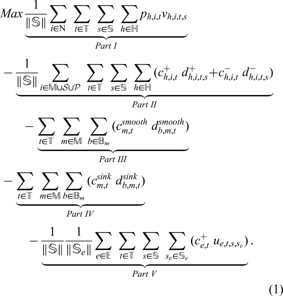

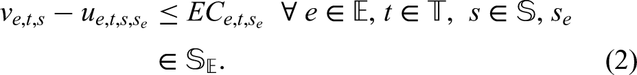
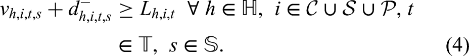
\begin{aligned} M a x \underset{P a r t I}{\underset{⏟}{\frac{1}{‖ S ‖} \sum_{i \in N} \sum_{t \in T} \sum_{s \in S} \sum_{h \in H} p_{h, i, t} v_{h, i, t, s}}} \\ - \underset{P a r t I I}{\underset{⏟}{\frac{1}{‖ S ‖} \sum_{i \in M \cup S \cup P} \sum_{t \in T} \sum_{s \in S} \sum_{h \in H} (c_{h, i, t}^{+} d_{h, i, t, s}^{+} + c_{h, i, t}^{-} d_{h, i, t, s}^{-})}} \\ - \underset{P a r t I I I}{\underset{⏟}{\sum_{t \in T} \sum_{m \in M} \sum_{b \in B_{m}} (c_{m, t}^{s m o o t h} d_{b, m, t}^{s m o o t h})}} \\ - \underset{P a r t I V}{\underset{⏟}{\sum_{t \in T} \sum_{m \in M} \sum_{b \in B_{m}} (c_{m, t}^{s i n k} d_{b, m, t}^{s i n k})}} \\ - \underset{P a r t V}{\underset{⏟}{\frac{1}{‖ S ‖} \frac{1}{‖ S_{e} ‖} \sum_{e \in E} \sum_{t \in T} \sum_{s \in S} \sum_{s_{e} \in S_{e}} (c_{e, t}^{+} u_{e, t, s, s_{e}})}} . \end{aligned}

(1)Part I of the objective function represents the discounted cash flow by accounting for the revenue from metal sales, the mining cost, the processing cost and other associated costs.

v_{h, i, t, s}

represent the amount produced that incurs a certain unit cost or revenue

p_{h, i, t}

. For example,

v_{h, i, t, s}

can represent the amount of copper produced by a mill in metric tonnes, and its corresponding

p_{h, i, t}

would be the copper selling price per tonne of copper. Part II represents the cost of deviating from the production target by applying penalties costs,

c_{h, i, t}^{+}

and

c_{h, i, t}^{-}

, to deviations,

d_{h, i, t, s}^{+}

and

d_{h, i, t, s}^{-}

, respectively. These penalties are discounted by geological discount rates (Dimitrakopoulos and Ramazan, 2004),

c_{h, i, t}^{+} = c_{h, i, 1}^{+} / (1 + r d)^{t}

. With the risk discount rate, the objective function aims to minimise the risk in early periods and defer the risk to later periods when more information is available. Parts III and IV are smoothing penalties and sink rate penalties to create a minable shape for the schedule. Part III ensures that the extraction sequence is practical in terms of adequate space for equipment access and movement. Extending the formulation of Goodfellow and Dimitrakopoulos (2016), Part V accounts for the additional penalties and related costs specific to equipment capacity, as applied to constraint the optimisation to mine and process materials given the simulated equipment capacities.

v_{e, t, s} - u_{e, t, s, s_{e}} \leq E C_{e, t, s_{e}} \forall e \in E, t \in T, s \in S, s_{e} \in S_{E} .

(2)To enforce the equipment capacity penalty, the additional equipment capacity constraints in equation (2) are applied in the extend model. For each location e with simulated equipment capacity

E C_{e, t, s_{e}}

, a penalty will incur when the production of material under orebody scenario s exceeding each equipment capacity scenario

s_{e}

, so the schedule will produce material respecting the equipment capacity.

Mineral complexes have many operational constraints and production targets, such as processing stream capacities and the acceptable ratio of different attribute grades of material in a processor. Equations (3) and (4) calculate the deviations from the upper and lower bounds of each production target at each location under every orebody scenario. 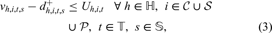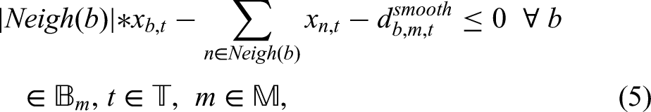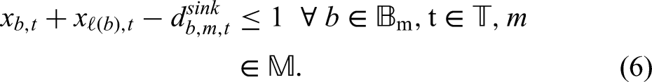By being penalised in the objective, the deviations, $d_{h, i, t, s}^{+}$ and $d_{h, i, t, s}^{-}$ , are controlled within upper $(U_{h, i, t})$ and lower $(L_{h, i, t})$ targets, respectively.

v_{h, i, t, s} - d_{h, i, t, s}^{+} \leq U_{h, i, t} \forall h \in H, i \in C \cup S \cup P, t \in T, s \in S,

(3)

v_{h, i, t, s} + d_{h, i, t, s}^{-} \geq L_{h, i, t} \forall h \in H, i \in C \cup S \cup P, t \in T, s \in S .

(4)To create a minable shape that allows equipment access, the smoothing constraints are included, as shown in equation (5).

N e i g h (b)

represents the neighbour of blocks surrounding block b within a predefined mining width, as shown in Figure 2. The smoothing penalty

d_{b, m, t}^{s m o o t h}

counts the number of blocks within

N e i g h (b)

that are not mined at the same period as b, like, then penalises the objective function. Similarly, the sink rate constraint, shown in equation (6), controls how deep the benches can be mined in one period.

ℓ (b)

represents the block overlay block b by the height of the predefined sink rate. For example, if the blocks are 10 m in height and the sink rate is 30 m, then

ℓ (b)

is the block 30 m above block b, and if they are mined at the same period t, penalty

d_{b, m, t}^{s i n k}

will incur.

| N e i g h (b) | * x_{b, t} - \sum_{n \in N e i g h (b)} x_{n, t} - d_{b, m, t}^{s m o o t h} \leq 0 \forall b \in B_{m}, t \in T, m \in M,

(5)

x_{b, t} + x_{ℓ (b), t} - d_{b, m, t}^{s i n k} \leq 1 \forall b \in B_{m}, t \in T, m \in M .

(6)

Figure 2.

Surrounding blocks in smoothing constraints.

The remaining constraints, such as capacity constraints, blending constraints, material type constraints, reserve, slope constraints and stockpile constraints are detailed by Goodfellow and Dimitrakopoulos (2016).

Solution approach

The simultaneous stochastic optimisation of a mining complex is challenging due to a large number of binary decision variables. Therefore, solution approaches that utilise commercial solvers are often infeasible. Metaheuristics and hyper-heuristics provide solution approaches to efficiently obtain near-optimal solutions for large stochastic optimisation models of mining complexes (Goodfellow and Dimitrakopoulos, 2016, 2017; Lamghari and Dimitrakopoulos, 2018). In this work, the solution approach is a combination of multi-neighbourhood simulated annealing with adaptive neighbourhood search, where the selection of heuristic is aided with reinforcement learning (RL) (Yaakoubi and Dimitrakopoulos, 2023).

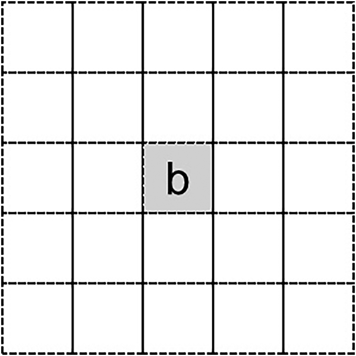
Starting with an initial solution, the simulated annealing algorithm (Kirkpatrick et al., 1983; Metropolis et al., 1953) iteratively explores neighbourhoods (Ribeiro and Laporte, 2012; Ropke and Pisinger, 2006) around the current solution. At each iteration, a new solution 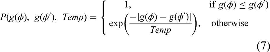$ϕ^{'}$ is generated by modifying either the extraction sequence decisions $(x ϵ ϕ)$ , destination decisions $(z ϵ ϕ)$ , or processing stream decisions $(y ϵ ϕ)$ of the current solution $ϕ$ using different heuristics. Then, instead of only accepting solutions that improve the objective function value, $g (ϕ)$ , deteriorating solutions might also be accepted based on a probabilistic acceptance criteria, as shown in equation (7). This probability is defined by an annealing temperature, $T e m p$ . Instead of using a fixed temperature, the annealing temperature will gradually cool down to zero based on cooling factors and cooling schedule (Goodfellow and Dimitrakopoulos, 2016). This mechanism balances the exploration, which prioritises searching through the solution space, and exploitation, focusing on improving the objective function.

g (ϕ)

(7)The improvement of the objective function value,

h_{i}

, depends on the selection of heuristics

i = 1, \dots, n,

(

S_{F} (h_{i})

where n in the number of low-level heuristics) used to modify the current solution. This selection of heuristics is governed by the learn-to-perturb (L2P) hyper-heuristic, which combines the multi-neighbourhood simulated annealing algorithm with RL (Yaakoubi and Dimitrakopoulos, 2023). L2P utilises a score function, shown in equation (8), where

h_{i}

represents the importance of heuristic

h_{i}

and the probability of this heuristic being selected (Yaakoubi and Dimitrakopoulos, 2023). The probability of each non-tabu heuristic

p_{i}

is computed by normalising the score function

p_{i} = S_{F} (h_{i}) / \sum_{k : H_{k}} S_{F} (h_{k})

. This score function is the weighted sum of two scores,

S_{1} (h_{i})

and

S_{2} (h_{i})

S_{1} (h_{i})

represents the recent performance of different heuristics (Lamghari and Dimitrakopoulos, 2018). A heuristic

h_{i}

is given higher

S_{1} (h_{i})

score if it improves solutions more efficiently per unit of execution time and it is given lower

S_{1} (h_{i})

score if it deteriorates the solution and consumes more execution time. However, the formulation of

S_{1} (h_{i})

requires expert knowledge, meaning it might require a different formulation if applied to different instances or during different stages of the optimisation process. To generalise the selection of heuristics across different instances,

S_{2} (h_{i})

is a score provided by an RL agent (Yaakoubi and Dimitrakopoulos, 2023). It predicts the performance of future iterations by learning from the past performance of different heuristics stored in a replay buffer. Compared to

S_{1} (h_{i})

, which only considers the recent performance,

S_{2} (h_{i})

is able to consider all perturbations and consecutive perturbations.

λ_{R L}

is used to control the contribution of the RL agent toward the final score

S_{F} (h_{i})

. When

λ_{R L} = 0

, the hyper-heuristic is not aided by the RL agent, referred as the baseline. The L2P approach refers to the hyper-heuristic aided by the RL agent, when

λ_{R L} > 0

. With the help of the RL agent, the heuristic selection process can learn from past experiences to be self-adaptive and can guide future searches through the solution space more efficiently. Figure 3 shows a comparison between the baseline hyper-heuristic and L2P approach (with contribution from the RL agent). For the same amount of execution time, the RL approach improves the solution efficiency

S_{F} (h_{i}) = (1 - λ_{R L}) S_{1} (h_{i}) + λ_{R L} S_{2} (h_{i}) .

(8)

Figure 3.

Evolution of objective function value, comparison of baseline heuristic selection (red line) and learn-to-perturb (L2P) approach (blue line).

Case study at a copper mining complex

Overview of the mining complex

The method of simultaneous stochastic optimisation described in the previous section is applied to an open-pit copper mining complex. As shown in Figure 4, the mining complex consists of two open-pit mines, mine 1 and mine 2, with, respectively, 414,108 and 157,749 blocks, which are 25 × 25 × 15 m³ in size. The main attributes of concern are copper total and copper soluble. Each block in the block model belongs to one of the four main material types, sulphide high grade, sulphide low grade, oxide and waste. Materials produced by the mines can be processed by different processing streams. Two products are produced by the mining complex, copper concentrate and copper cathodes. As shown in Figure 4, Mill 1, Mill 2 and Mill 3 receive high-grade sulphide material from mines 1 and 2 after materials are crushed by their corresponding crushers and produce copper concentrate as a product. The oxide leach pad takes oxide materials from both mines after the oxide material is crushed by the oxide crusher and produces copper cathodes. The sulphide leach pad takes low-grade material from both mines and produces copper cathode as a product. The sulphide leach pad requires the ratio of copper total and copper soluble to be within its operational limit.

Figure 4.

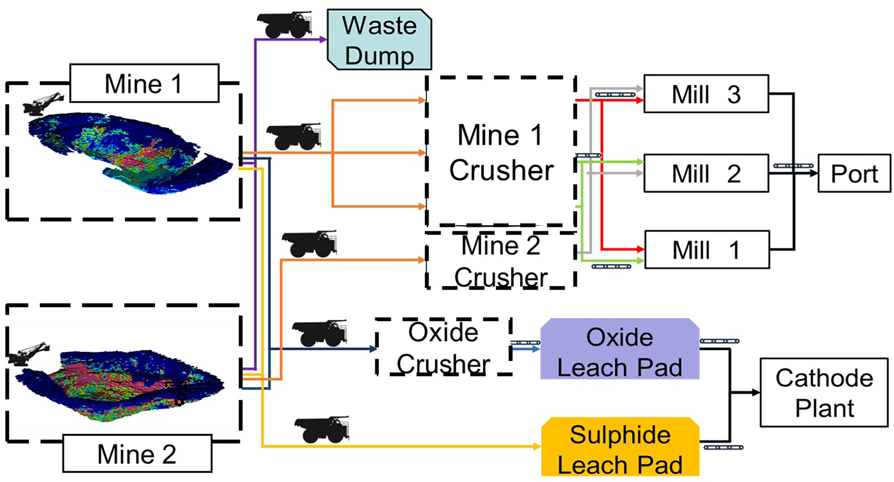
Copper mining complex, with five locations for modelling equipment uncertainty (highlighted in dash line).

The long-term strategic plan currently used in the mining complex is based on the conventional sequential optimisation approach that uses estimated orebodies as input. First, the extraction sequences of each mine are optimised separately based on bench design. Then the destination policy is determined based on the cut-off policy and materials produced by the extraction sequences of both mines. Lastly, another optimisation process is used to maximise the utilisation of each processing stream. The use of estimated orebodies ignores the geological uncertainties presented in the deposits, and the use of fixed equipment capacity ignores the equipment performance uncertainty.

The simultaneous stochastic optimisation framework previously described addresses the disadvantages of the sequential conventional optimisation approach. First of all, the stochastic framework considers every component in the mining complex simultaneously to capture the synergies among components. By optimising the extraction sequence, destination policy and processing stream decisions of the two mines at the same time, the downstream operation will not be misled by predetermined extraction sequences. Also, the stochastic framework incorporates both supply uncertainty for the two mines and equipment uncertainty for multiple equipment locations. The blending constraint is considered throughout the optimisation process.

Modelling equipment uncertainty

Equipment capacities can be simulated at different components in a mining complex to represent the uncertainties associated with the different equipment. For modelling realistic equipment uncertainty, Monte Carlo simulation methods are used. Equipment simulation starts with the historical daily production data of each type of equipment. Then, based on the historical production data, the empirical distribution of the equipment performance can be built. Then, by sampling this distribution 365 times and grouping these daily productivities, the annual productivity of a single piece of equipment can be simulated.

Figure 5 shows an example of producing multiple simulations for one type of equipment. The blue line represents the empirical distribution constructed from historical production data, and the set of green lines represents multiple sampling results conducted on the empirical distribution. The figure is presented as a probability distribution graph where the horizontal axis presents the tonnage per day (tpd) productivity achieved by this type of equipment and the vertical one the frequency of occurrence. Figure 5 demonstrates that the equipment simulations are able to reproduce the historical data distribution.

Figure 5.

Equipment simulation of type A trucks.

After simulating the annual productivity of each type of equipment, then combined with an equipment plan, which shows how many trucks and shovels of equipment are being used in the mine, the total production capacity of an equipment fleet, such as truck fleet and shovel fleet, can be computed.

The production of the mining complex is limited by not only the equipment capacity in the mines for trucks and shovels, but also by the crusher capacity. Therefore, the modelling of equipment uncertainty is conducted at five locations in the mining complex. As shown in Figure 4, the uncertainty of the mining capacities of two mines is modelled using truck and shovel uncertainty. Three crushers are used to crush materials from mine 1 before sending them to the mills, one crusher for crushing mine 2 materials for the mills, and one crusher for crushing oxide material from both mines for oxide leach.

For the mining capacities of the two mines, equipment simulations for each type of truck and shovel will be produced, and then, based on the equipment plan for each mine, the total simulated mining rate can be computed. Figure 6 shows the result of the equipment simulation of four types of trucks. As shown in Figure 6, for each type of truck, the equipment simulations (green lines) reproduce the historical data distribution (blue lines). Similarly, Figure 7 shows that, for each type of shovel, the equipment simulations (green lines) reproduce the historical data distribution (blue lines).

Figure 6.

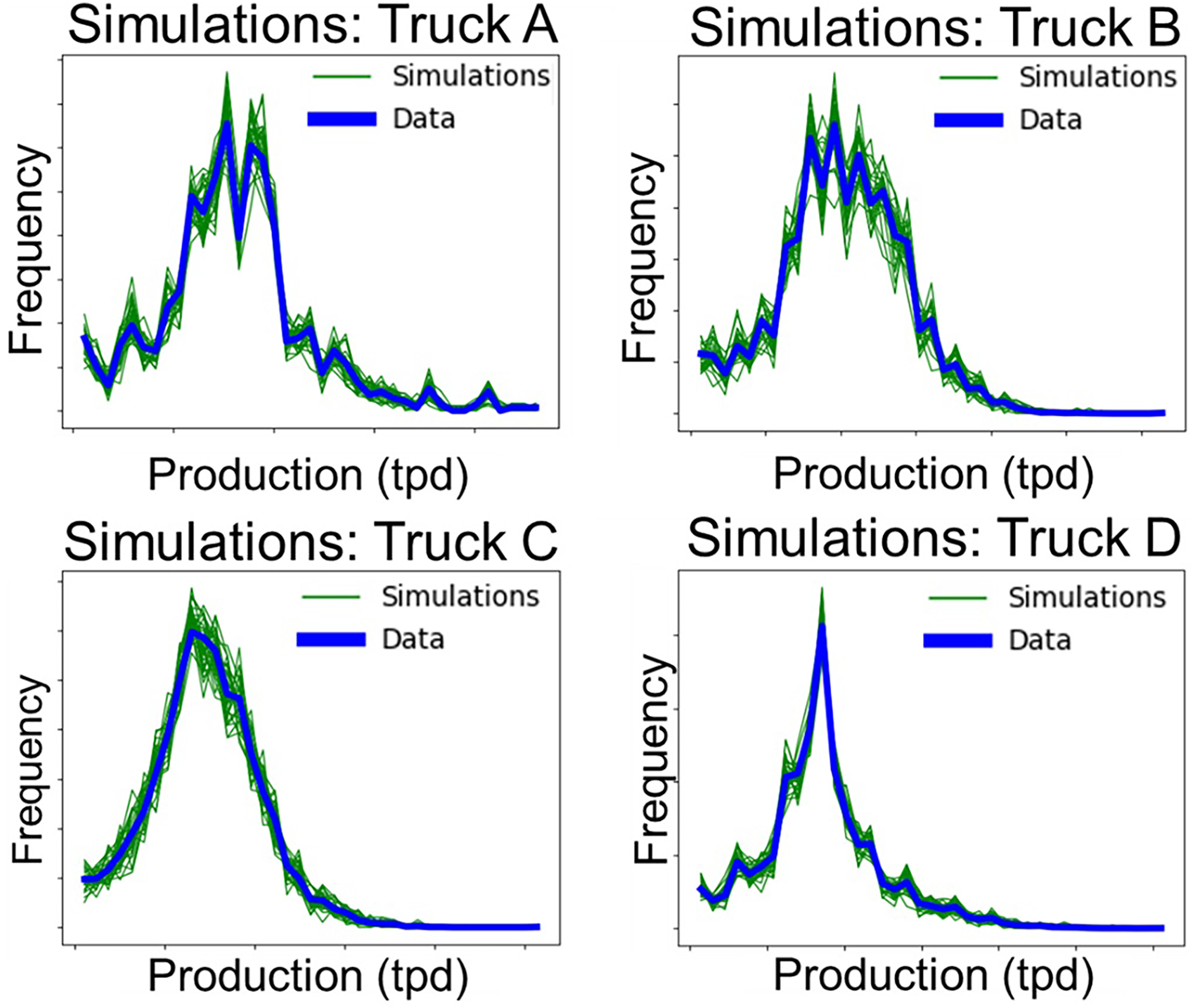
Equipment simulations for four types of trucks.

Figure 7.

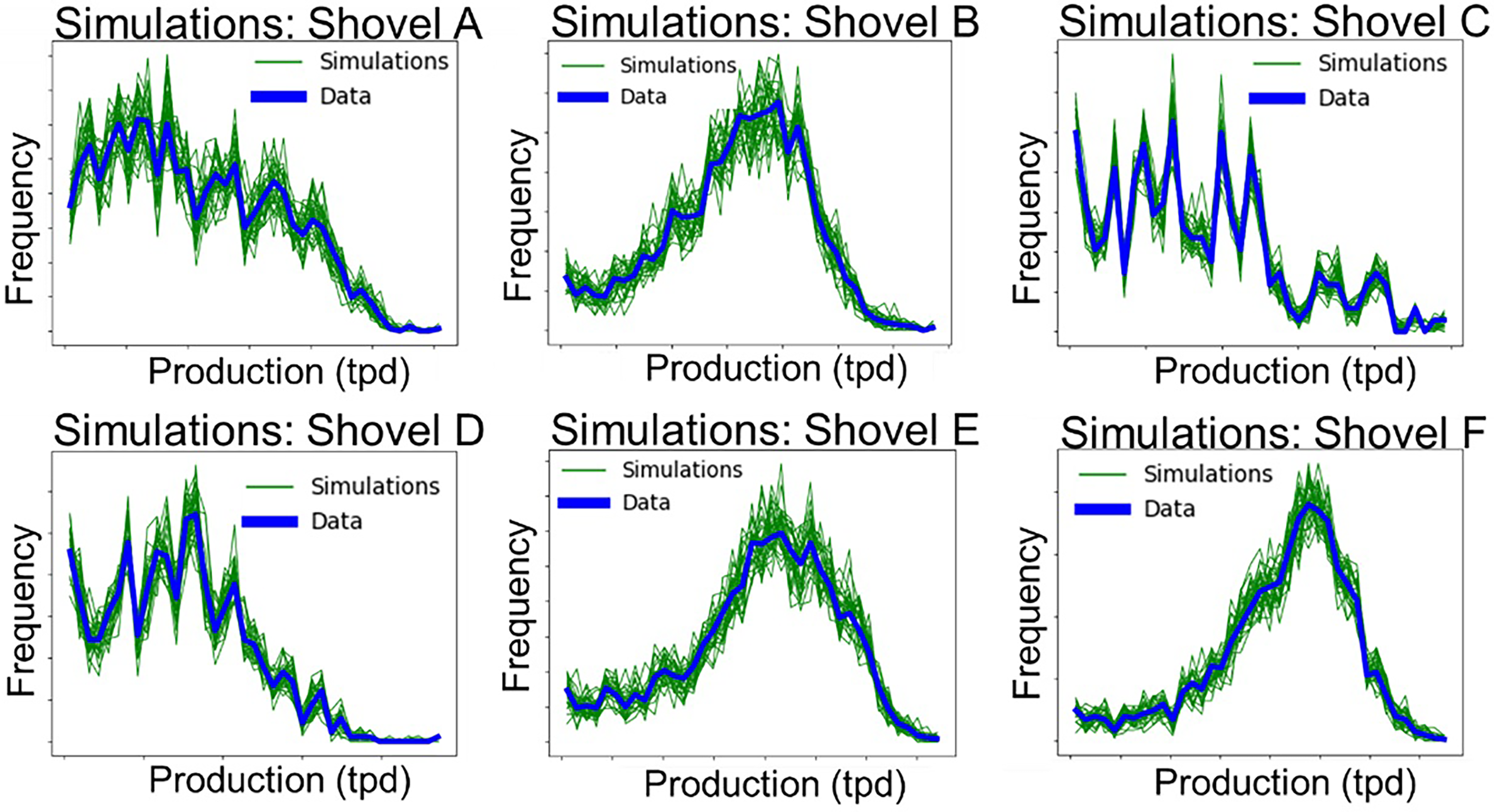
Equipment simulation for six types of shovels.

For simulating the crusher capacity, Figure 8 shows a simulation for five crushers and, similarly to trucks and shovels, simulations reproduce the historical data distribution.

Figure 8.

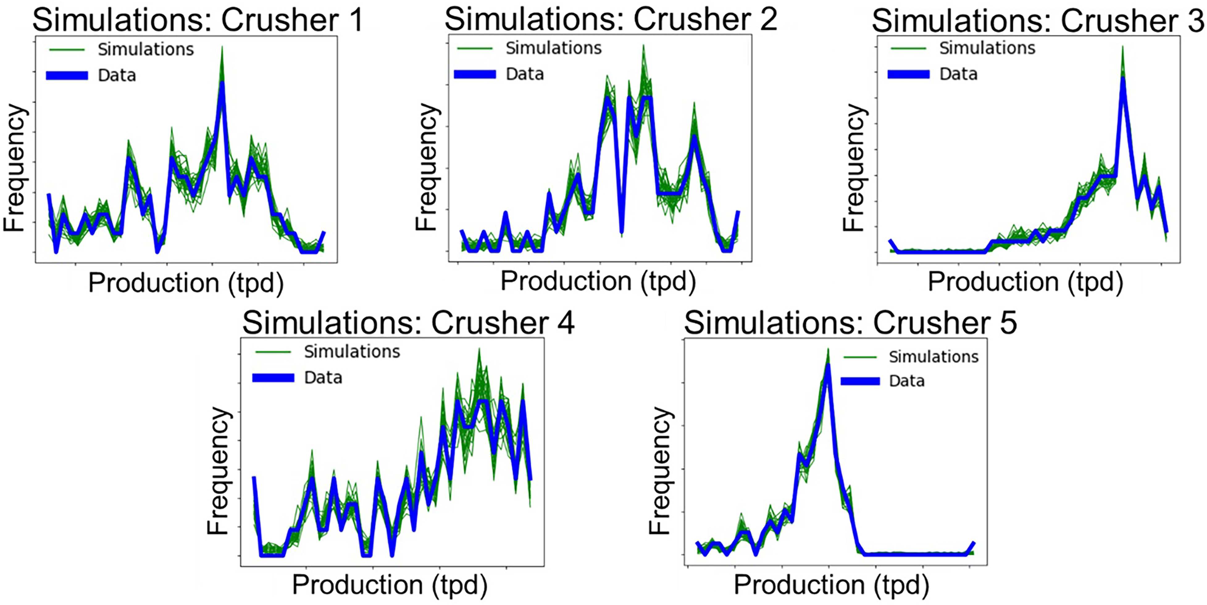
Equipment simulation for five crushers.

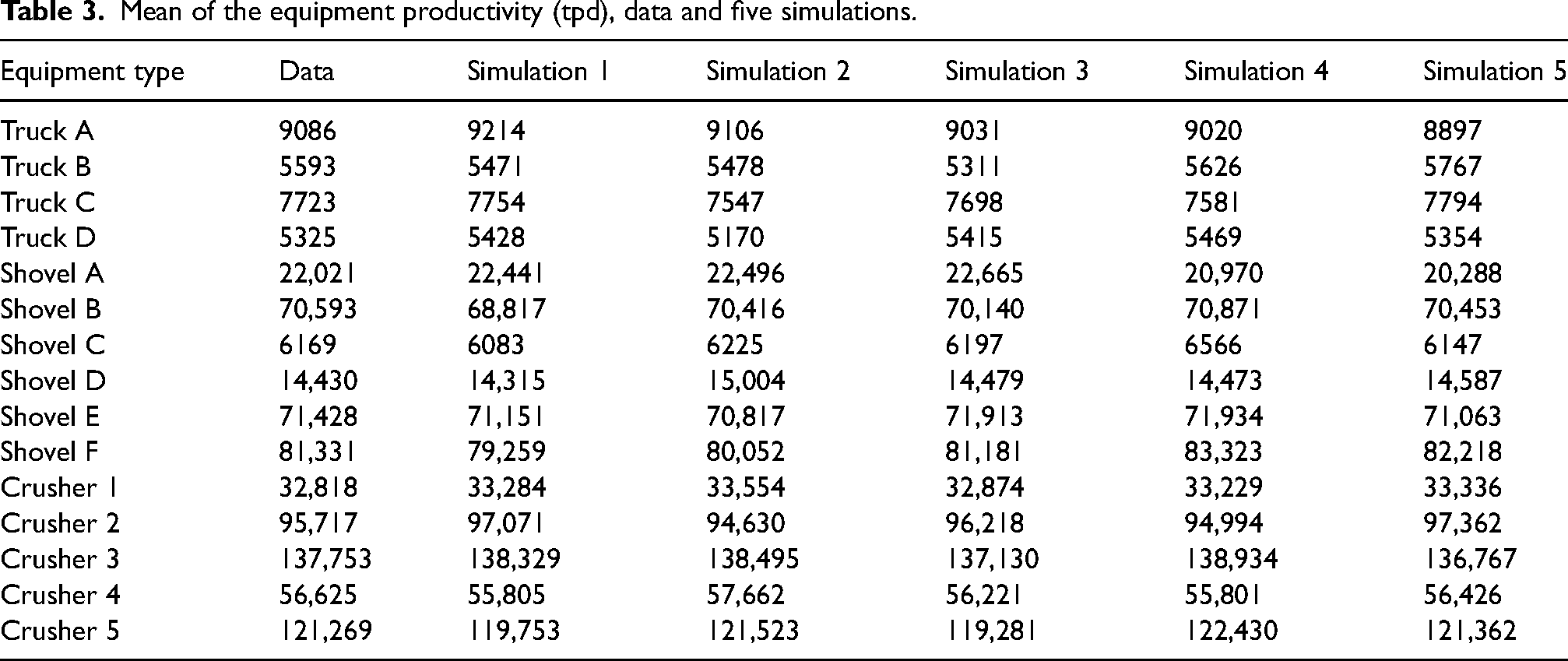
To validate the equipment simulations, statistical comparisons between the simulated and the data productivity are shown in Tables 3 and 4. Table 3 shows the mean of the historical productivity data of each type of equipment, comparing to the five simulations, while Table 4 shows the standard deviation.

Table 3.

Mean of the equipment productivity (tpd), data and five simulations.

Equipment type	Data	Simulation 1	Simulation 2	Simulation 3	Simulation 4	Simulation 5
Truck A	9086	9214	9106	9031	9020	8897
Truck B	5593	5471	5478	5311	5626	5767
Truck C	7723	7754	7547	7698	7581	7794
Truck D	5325	5428	5170	5415	5469	5354
Shovel A	22,021	22,441	22,496	22,665	20,970	20,288
Shovel B	70,593	68,817	70,416	70,140	70,871	70,453
Shovel C	6169	6083	6225	6197	6566	6147
Shovel D	14,430	14,315	15,004	14,479	14,473	14,587
Shovel E	71,428	71,151	70,817	71,913	71,934	71,063
Shovel F	81,331	79,259	80,052	81,181	83,323	82,218
Crusher 1	32,818	33,284	33,554	32,874	33,229	33,336
Crusher 2	95,717	97,071	94,630	96,218	94,994	97,362
Crusher 3	137,753	138,329	138,495	137,130	138,934	136,767
Crusher 4	56,625	55,805	57,662	56,221	55,801	56,426
Crusher 5	121,269	119,753	121,523	119,281	122,430	121,362

Table 4.

Standard deviation of the equipment productivity (tpd), data and five simulations.

Equipment type	Data	Simulation1	Simulation2	Simulation3	Simulation4	Simulation5
Truck A	4949	5104	4888	4980	4862	4978
Truck B	4045	4154	4024	4079	4030	3997
Truck C	4435	4410	4409	4527	4275	4360
Truck D	4740	4682	4786	4823	4723	4712
Shovel A	28,430	28,141	28,153	29,419	27,879	27,939
Shovel B	38,678	38,998	39,812	39,226	39,564	38,150
Shovel C	10,589	10,441	10,567	10,520	11,053	10,746
Shovel D	18,701	18,935	19,137	18,219	18,492	18,947
Shovel E	36,358	36,552	36,291	35,240	37,451	37,232
Shovel F	31,743	33,036	32,426	30,991	31,308	30,871
Crusher 1	15,616	15,533	15,358	15,950	15,532	15,256
Crusher 2	31,487	30,598	31,567	32,338	31,823	31,562
Crusher 3	31,393	30,232	30,300	34,282	29,757	33,009
Crusher 4	24,046	24,625	24,077	24,249	24,325	23,477
Crusher 5	47,405	48,613	47,090	48,737	46,734	46,479

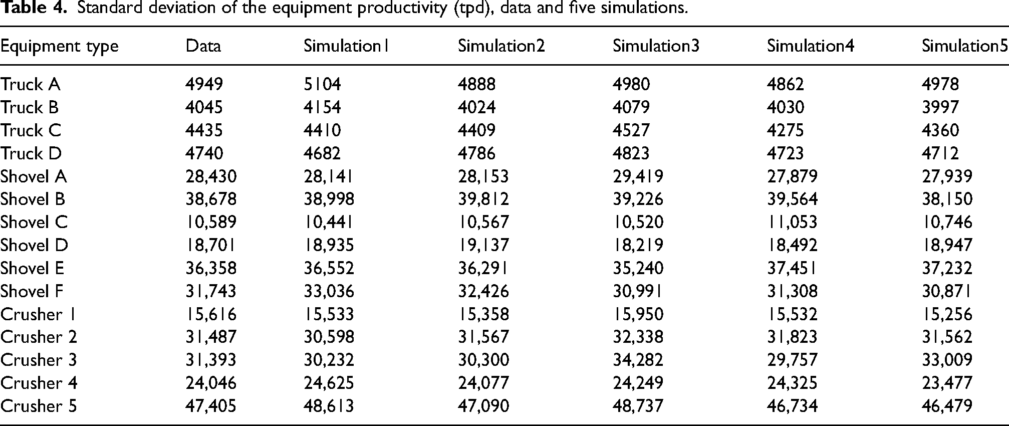
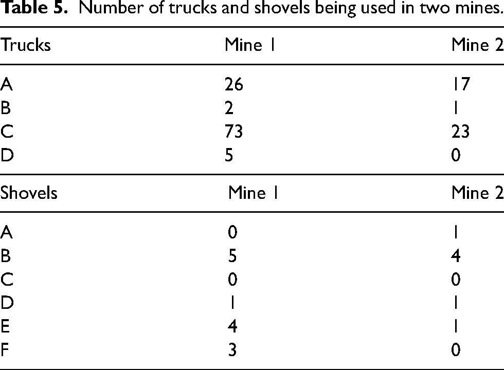
Table 5 shows the equipment plan for each mine, the equipment plan shows how many trucks and shovels of each type are being used in the mine. Therefore, using this equipment plan and the previous simulated productivity of each type of equipment, the total simulated capacity can be computed for the shovel fleet and truck fleet for mines 1 and 2. The sum of the simulated productivities of Crushers 1, 2 and 3 will be used as the simulated capacity of the mine 1 crusher. The simulated productivities of Crusher 4 will be used as the simulated capacity of the oxide crusher. The simulated productivities of Crusher 5 will be used as the simulated capacity of the mine 2 crusher.

Table 5.

Number of trucks and shovels being used in two mines.

Trucks	Mine 1	Mine 2
A	26	17
B	2	1
C	73	23
D	5	0

Shovels	Mine 1	Mine 2
A	0	1
B	5	4
C	0	0
D	1	1
E	4	1
F	3	0

Parameters

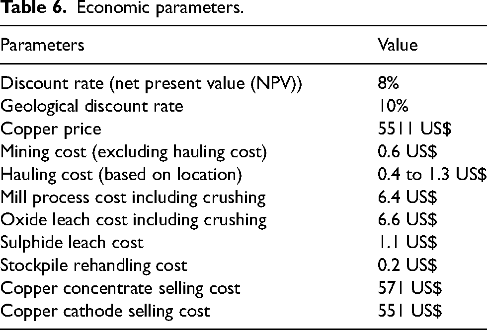
The case study of simultaneous stochastic optimisation for this copper mining complex requires two sets of parameters. The set of parameters includes (i) the economic and (ii) the operational parameters associated with the mining operation. These are summarised in Table 6 for the economic parameters and Table 7 for the operational parameters. Due to confidentiality reasons, the parameters listed in both tables are scaled.

Table 6.

Economic parameters.

Parameters	Value
Discount rate (net present value (NPV))	8%
Geological discount rate	10%
Copper price	5511 US$
Mining cost (excluding hauling cost)	0.6 US$
Hauling cost (based on location)	0.4 to 1.3 US$
Mill process cost including crushing	6.4 US$
Oxide leach cost including crushing	6.6 US$
Sulphide leach cost	1.1 US$
Stockpile rehandling cost	0.2 US$
Copper concentrate selling cost	571 US$
Copper cathode selling cost	551 US$

Table 7.

Operational parameters.

Parameters	Value
Mining width	200 m
Sink rate	100 m
Slope angle	37° (mine 1)	45° (mine 2)
Mill 1 recovery	83%
Mill 2 recovery	80%
Mill 3 recovery	82.6%
Oxide reach recovery	65%
Sulphide leach recovery	27%
Number of blocks	414,108 (mine 1)	157,749 (mine 2)
Number of periods	8

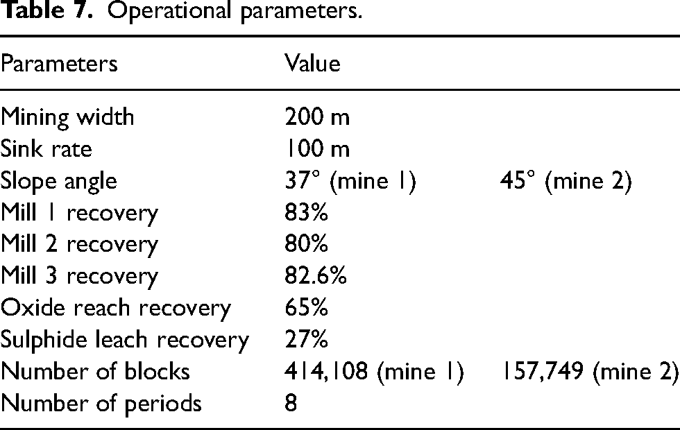
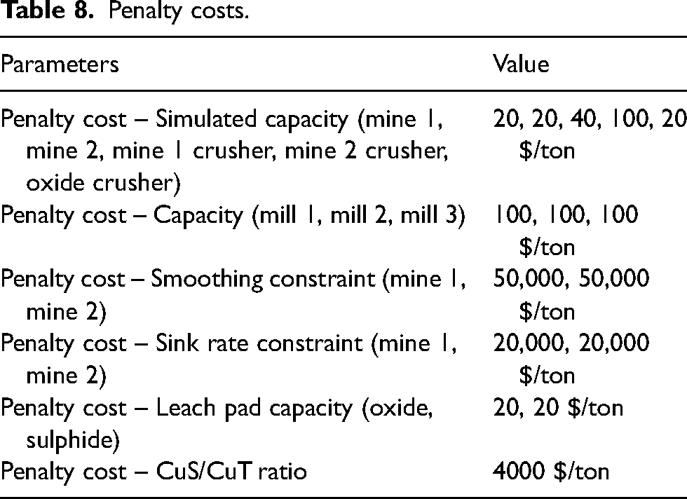
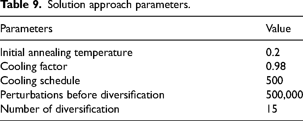
Table 6 summarises the costs associated with the mining operation and the price of metal produced. Table 7 includes the mining width, sink rate and slope angle limitation, as well as fixed recovery rates, for different processing streams. The number of blocks considered for this application is 414,108 for mine 1 and 158,749 for mine 2. Therefore, the total number of decision variables exceeds 4.5 million and the number of constraints exceeds 9 million. The penalty costs associated with the objective function are listed in Table 8. They are determined based on a trial and error process to achieve an acceptable level of technical risk for different production targets and the economic outcome. The second set is related to the solution algorithm. The parameters used for the solution approach are summarised in Table 9. The initial temperature specifies the probability of the simulated annealing algorithm accepting deteriorating solutions at the first diversification. The cooling factor, cooling schedule and the number of perturbations before diversification decide what proportions of the optimisation are spent searching in the solution space and improving the solution. The perturbations before diversification and the number of diversifications are specific to the length of optimisation.

Table 8.

Penalty costs.

Parameters	Value
Penalty cost – Simulated capacity (mine 1, mine 2, mine 1 crusher, mine 2 crusher, oxide crusher)	20, 20, 40, 100, 20 $/ton
Penalty cost – Capacity (mill 1, mill 2, mill 3)	100, 100, 100 $/ton
Penalty cost – Smoothing constraint (mine 1, mine 2)	50,000, 50,000 $/ton
Penalty cost – Sink rate constraint (mine 1, mine 2)	20,000, 20,000 $/ton
Penalty cost – Leach pad capacity (oxide, sulphide)	20, 20 $/ton
Penalty cost – CuS/CuT ratio	4000 $/ton

Table 9.

Solution approach parameters.

Parameters	Value
Initial annealing temperature	0.2
Cooling factor	0.98
Cooling schedule	500
Perturbations before diversification	500,000
Number of diversification	15

Results of stochastic optimisations incorporating joint supply and equipment uncertainty

The result of the stochastic optimisation incorporating both supply and equipment uncertainty will be presented in this section and is referred to as the ‘joint uncertainty’ case. To provide a comparison, the result of only incorporating the supply uncertainty, with constant equipment capacity, will be included and referred to as the ‘supply uncertainty’ case. Therefore, the comparison will demonstrate the effect of including both equipment uncertainty and supply into the optimisation framework.

Figure 9 shows the risk profile of the amount of material produced by mines 1 and 2. Black lines show the simulated equipment capacities. As shown in Figure 9(a), the joint stochastic case (blue lines) utilises more of the simulated capacity of the equipment in mine 1 compared to the supply case (green lines). Mine 2 shows a similar result in Figure 9(b) where the joint stochastic case utilises more of the capacity of the truck fleet and shovel fleet in the mine at years 1 and 4.

Figure 9.

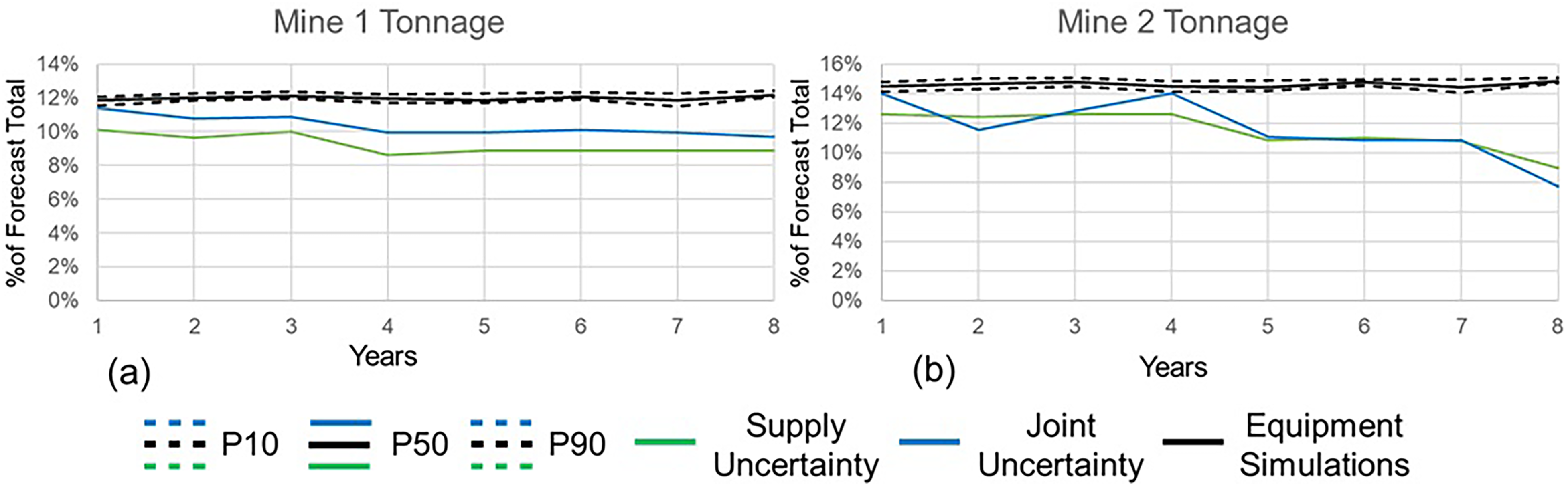
Mine 1 tonnage and mine 2 tonnage for supply uncertainty and joint uncertainty case.

After the materials are extracted from the mine, they are sent to the crushers for size reduction. The result of crusher production is shown in Figure 10. Figure 10(a) shows that the supply uncertainty case is trying to produce slightly more material than what mine 1 crusher can handle. The risk profile for mine 1 shows the crusher production for supply uncertainty would exceed the equipment capacity. In comparison, the joint uncertainty case respects the simulated capacity better than the supply uncertainty case. Although the stochastic optimisation tries to push the mine 1 crusher production as much as possible, it still respects the simulated capacity. The supply uncertainty case is likely to send more material to the crusher exceeding the crusher capacity. In another words, the joint case is expected to produce a more realisable schedule as it complies with the simulated production capacity. This can also explain the previous result in which the equipment capacity in the mines was not fully utilised. The mine 1 crusher can only handle a limited amount of high-grade ore from mine 1 based on the simulations. The optimiser is able to identify that the mining complex is restricted by the crusher capacities. For the mine 2 crusher shown in Figure 10(b), the production of both supply and joint uncertainty cases respect the simulated capacity. However, the joint uncertainty case produces more material compared to the supply case, processing 11% more material. The joint uncertainty case is able to utilise more capacity of the mine 2 crushers. For the oxide crusher shown in Figure 10(c), a similar result is also observed where the production risks exceeding the equipment capacity at years 2, 3, 6 and 7 for the supply uncertainty case. However, the joint uncertainty case will be able to respect these limitations.

Figure 10.

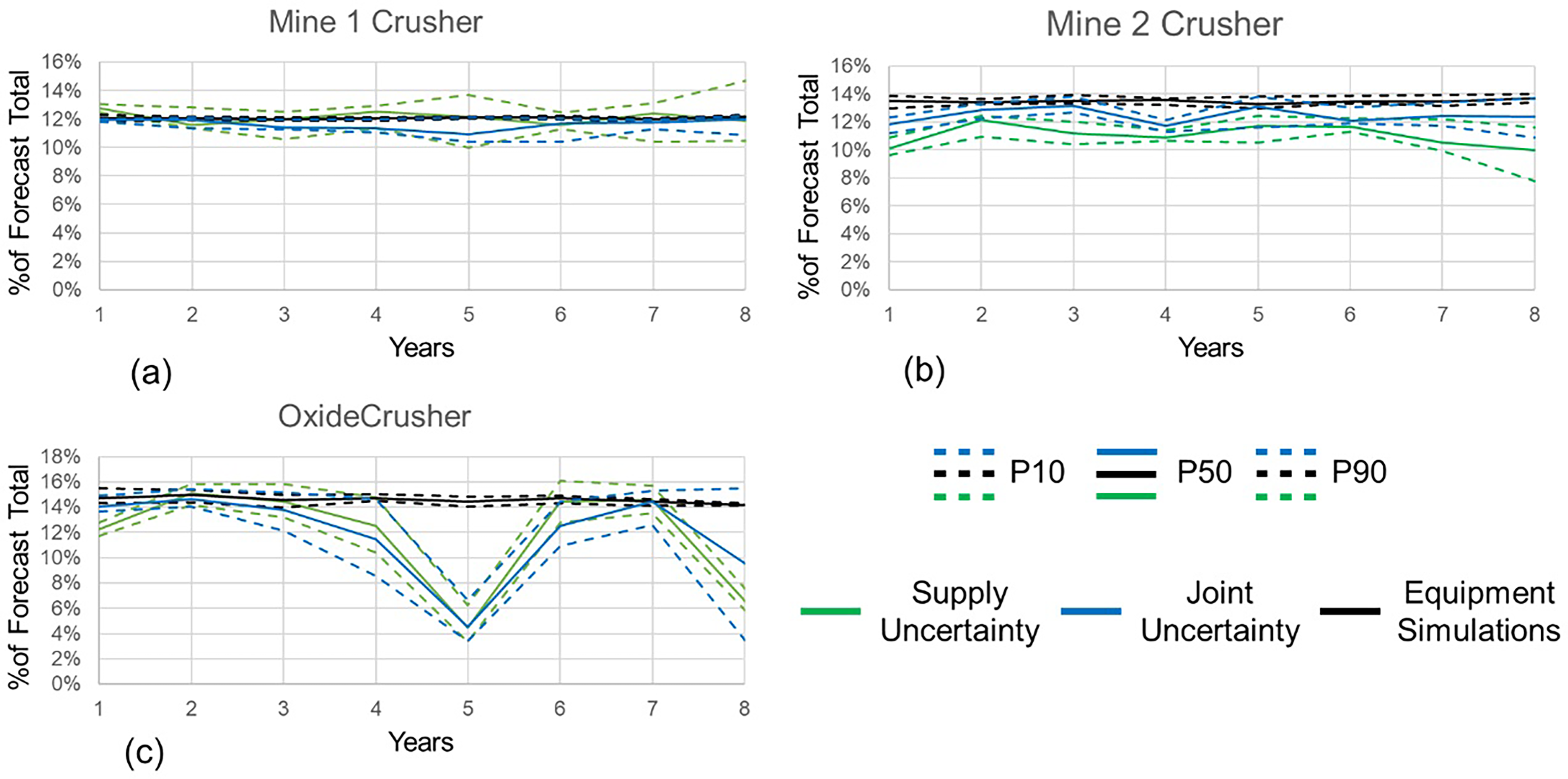
Material processed by mine 1 crusher (a), mine 2 crusher (b) and oxide crusher (c).

The results of copper metal recovered from Mills 1, 2 and 3 are shown in Figure 11. Figure 11(a) and (c) shows that, for the joint uncertainty case, Mills 1 and 3 will recover ∼ 11% and 16% more copper in the first 2 years and a similar amount in later years. Mill 2 will recover 8% less than the supply uncertainty case in the first 2 years. As for the copper recovered from the leach pad shown in Figure 12, the joint uncertainty case gives different results compared to the supply uncertainty schedule. For both oxide leach and sulphide leach, the joint uncertainty case shows a similar amount of copper is recovered at the earlier periods and slightly more copper at later periods, compared to the supply uncertainty case.

Figure 11.

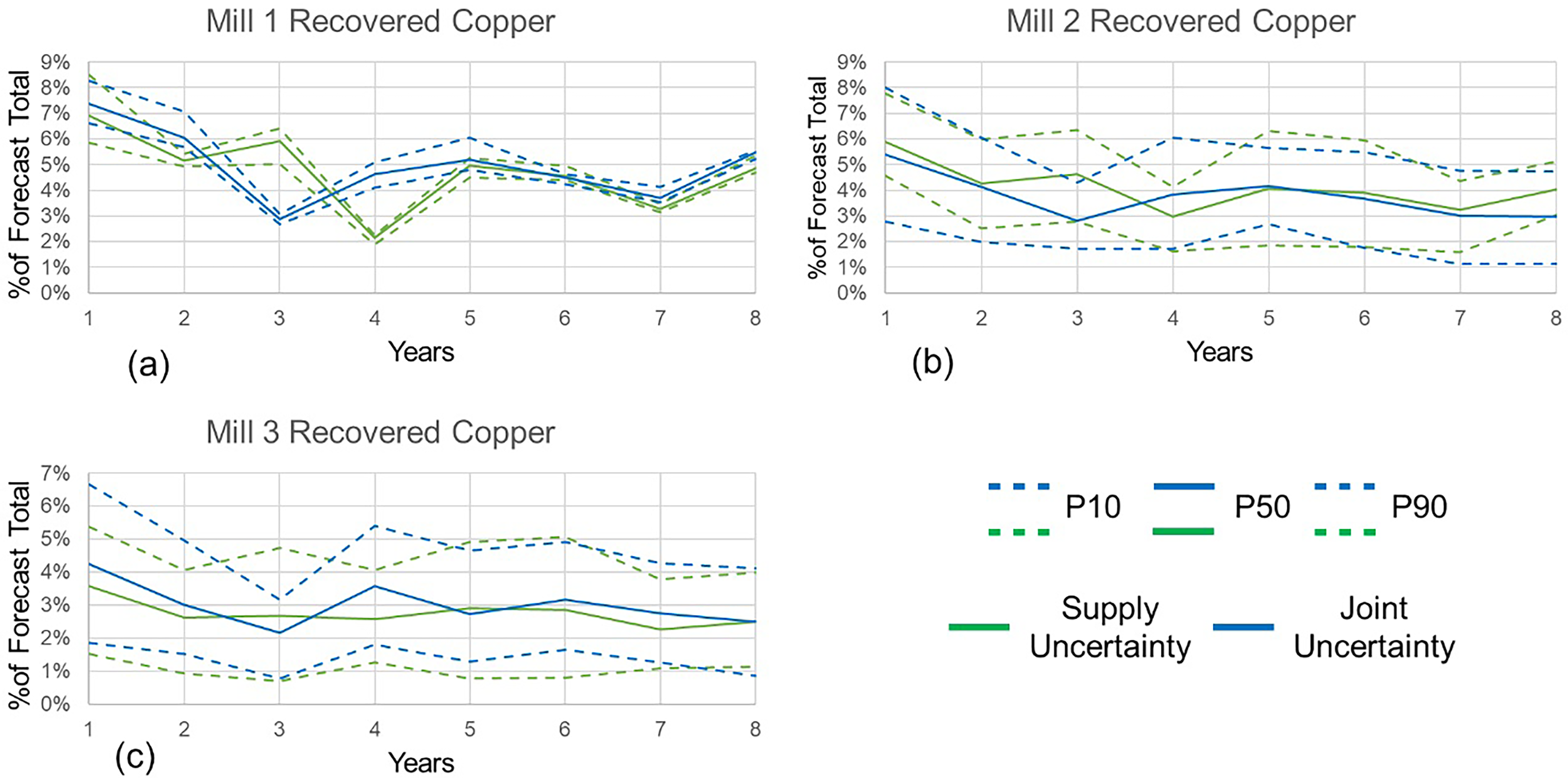
Copper recovered by mill 1 (a), mill 2 (b) and mill 3 (c).

Figure 12.

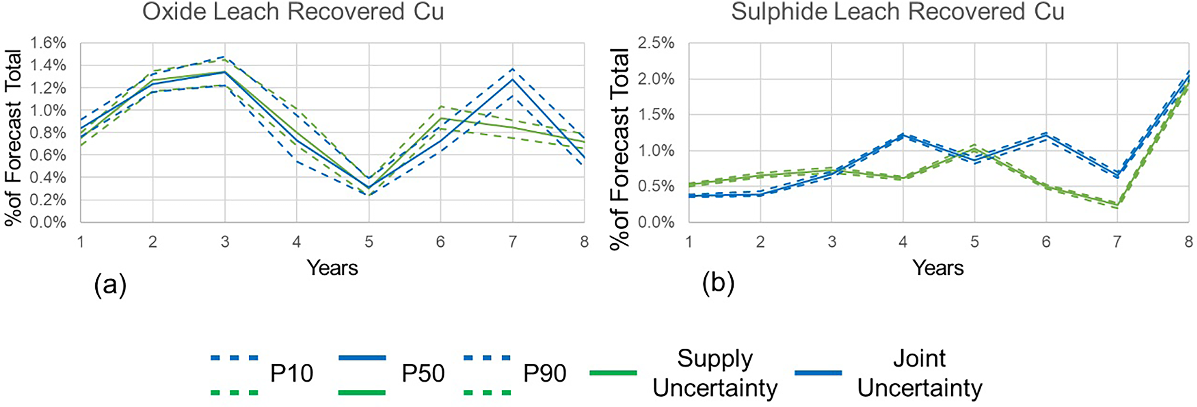
Copper recovered by oxide leach (a) and sulphide leach (b).

For waste management, Figure 13 shows the waste tonnages and the copper content in the waste material. The joint uncertainty case shows that it extracts about 13% more waste compared to the supply uncertainty case. However, the copper content in the waste material is less than in the supply case. The joint uncertainty case is capable of improving the waste management in earlier periods.

Figure 13.

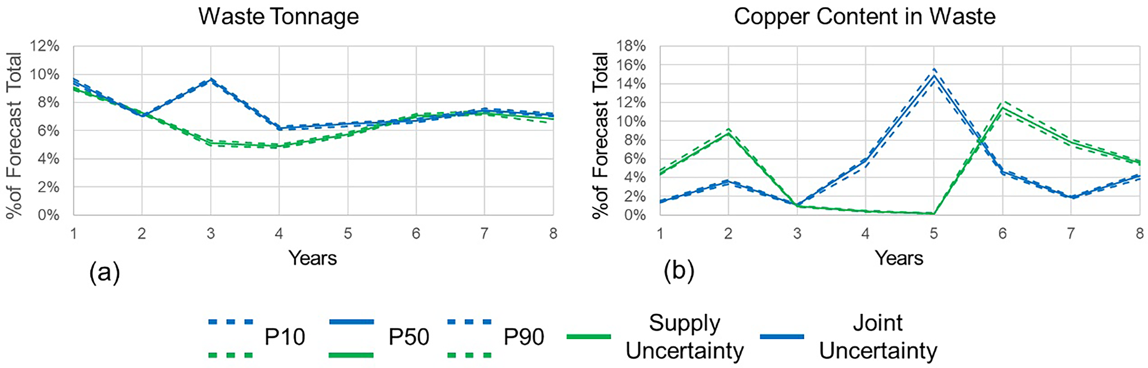
Waste management.

To demonstrate more clearly the amount of metal recovered, the amount of copper recovered by mills and leach-pads are summed up separately in Figure 14. As shown in Figure14(a), the mill recovered the majority of the copper metal. About 89% of copper is recovered by the mill, and about 11% is recovered by the leach pads. The joint uncertainty case recovers about 5% more metal in the first year, and a similar amount of metal in later years, as shown in Figure 14(a). For the leach pads, Figure 14(b) shows that the stochastic plan recovers a similar amount of copper in earlier years and slightly more copper in later years. As a result, Figure 14(c) shows that the joint uncertainty case can generate a 2% higher NPV compared to what the supply uncertainty case is capable of delivering under equipment uncertainty at the end of eight periods. The production schedules for the two cases are shown in Figures 15 and 16, where each period is represented by a distinct colour gradient from blue in period 1 to red in period 8. For mine 1, the production schedule of the joint uncertainty case extracts slightly more material compared to the supply uncertainty case. This result is consistent with the previous observation: namely, that considering equipment uncertainty improves the use of equipment.

Figure 14.

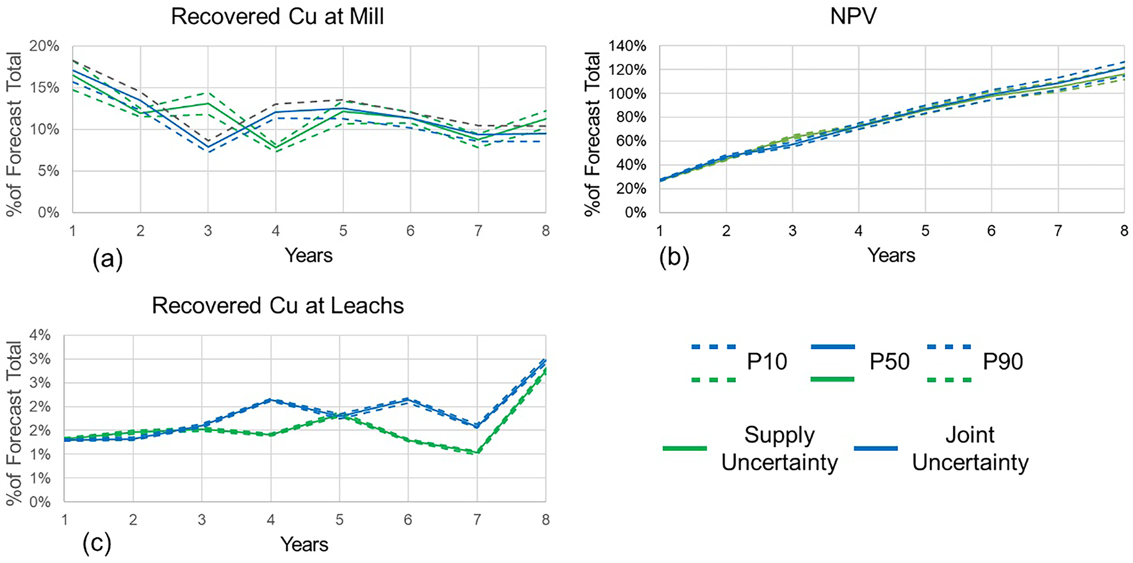
Total recovered copper from mills (a) and from leach pads (b), and net present value (NPV) of the mining complex (c).

Figure 15.

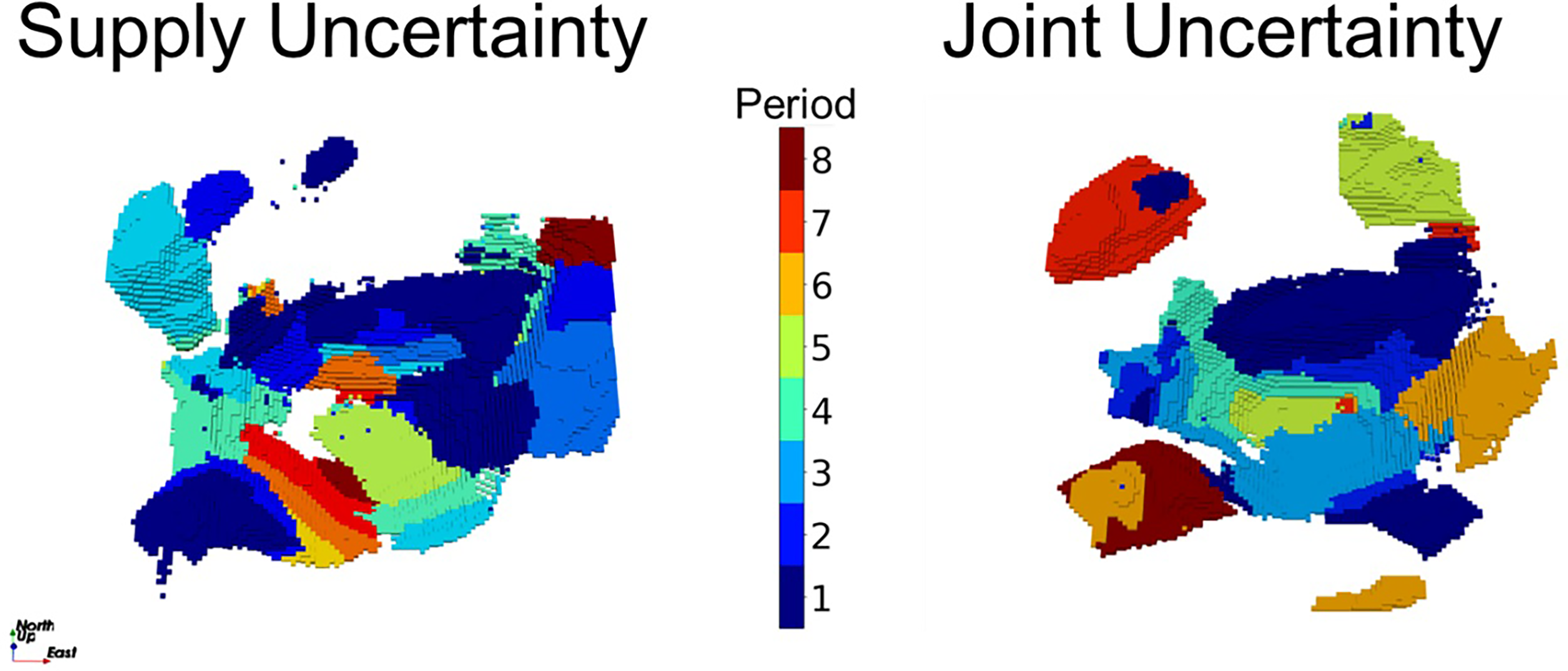
Plan-view of mine 1 production schedule for supply uncertainty case and joint uncertainty case.

Figure 16.

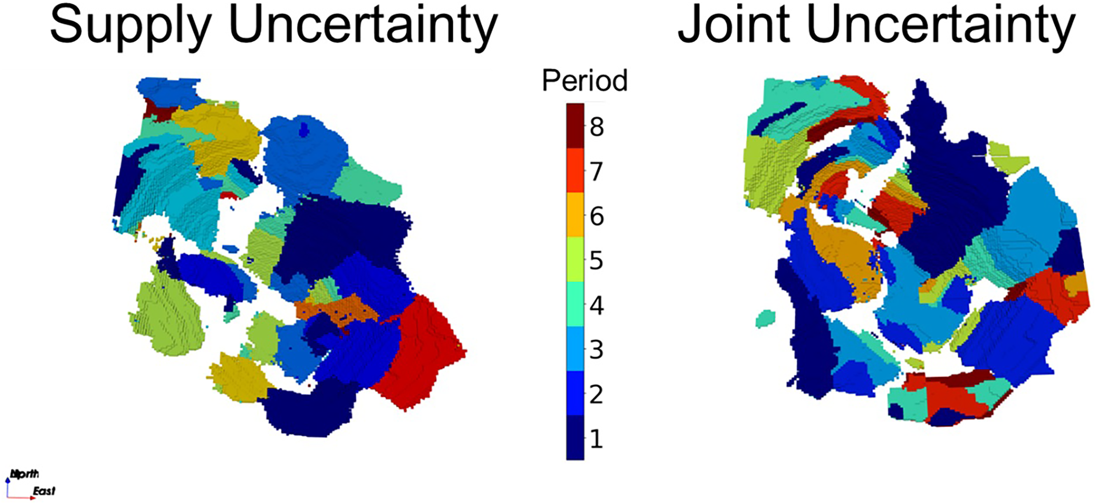
Plan-view of mine 2 production schedule for supply uncertainty case and joint uncertainty case.

In summary, the joint uncertainty case results in a better production schedule with higher utilisation of equipment that better respects the equipment capacity. Also, it can achieve a slightly higher NPV by recovering more copper at earlier periods. This improvement is in addition to the improvement achieved by incorporating supply uncertainty into simultaneous stochastic optimisation compared to the conventional method.

Conclusions

This article extends the previous simultaneous stochastic optimisation framework of mining complexes to include equipment uncertainty and related constraints. The application at a copper mining complex demonstrates the practical aspects of integrating joint supply and equipment uncertainties. The uncertainty of equipment productivity is captured by simulations based on historical production data using Monte Carlo simulations. By integrating equipment uncertainty, in addition to geological (supply) uncertainty, the optimisation process respects the simulated equipment capacity, resulting in pragmatic and realistic life-of-asset production schedules. In the case study, the joint uncertainty production schedule produces 5% more copper for the mills in the first year, although the risk profiles show more fluctuations across multiple periods compared to the schedule where only supply uncertainty is considered. The leach pads also show higher copper production in later years. Consequently, the proposed extended stochastic schedule now reflects and manages risk regarding equipment productivity, and achieves a 2% higher NPV compared to the schedule that considers only supply uncertainty, while it is also capable of improving waste management in the earlier years.

Future research directions could consider haul cycles in the optimisation process. Another important avenue could be including factors such as block depth and distance from the mining site, which influence truck productivity and cost structure. Evaluating the feasibility of investing in an additional crusher to alleviate production constraints mentioned previously may significantly impact overall productivity and profitability. In addition, various operating modes can be explored for the mill, such as including options with higher recovery but lower throughput. Additional case studies and comparisons would also be valuable in terms of providing an understanding of the effects of different equipment configurations in mining operations.

Footnotes

Declaration of conflicting interests

The author(s) declared no potential conflicts of interest with respect to the research, authorship, and/or publication of this article.

Funding

The authors disclosed receipt of the following financial support for the research, authorship, and/or publication of this article: The work in this article was funded by the National Sciences and Engineering Research Council (NSERC) of Canada CRD Grant 500414-16 and NSERC Discovery Grant 239019, the industry consortium members of McGill's COSMO Stochastic Mine Planning Laboratory (AngloGold Ashanti, AngloAmerican, BHP, De Beers, IAMGOLD, Kinross, Newmont and Vale); and the Canada Research Chairs Program.

References

Both

Dimitrakopoulos

(2020) Joint stochastic short-term production scheduling and fleet management optimization for mining complexes. Optimization and Engineering 21: 1717–1743.

Del Castillo

Dimitrakopoulos

(2019) Dynamically optimizing the strategic plan of mining complexes under supply uncertainty. Resources Policy 60: 83–93.

Dimitrakopoulos

Farrelly

Godoy

(2002) Moving forward from traditional optimization: Grade uncertainty and risk effects in open-pit design. Mining Technology 111(1): 82–88.

Dimitrakopoulos

Lamghari

(2022) Simultaneous stochastic optimization of mining complexes – mineral value chains: An overview of concepts, examples and comparisons. International Journal of Mining, Reclamation and Environment 36(6): 443–460.

Dimitrakopoulos

Ramazan

(2004) Uncertainty-based production scheduling in open pit mining. Society for Mining, Metallurgy, and Exploration 316: 106–112.

Dowd

(1994) Risk assessment in reserve estimation and open-pit planning. Transactions of the Institution of Mining and Metallurgy-Section A-Mining Industry 103: 148–154.

Dowd

(1997) Risk in minerals projects: Analysis, perception and management. Transactions of the Institutions of Mining and Metallurgy Section A-Mining Technology 106: A9–A18.

Farmer

(2017) Stochastic Mining Supply Chain Optimization: A Study of Integrated Capacity Decisions and Pushback Design under Uncertainty . McGill University.

Goodfellow

Dimitrakopoulos

(2016) Global optimization of open pit mining complexes with uncertainty. Applied Soft Computing 40: 292–304.

10.

Goodfellow

Dimitrakopoulos

(2017) Simultaneous stochastic optimization of mining complexes and mineral value chains. Mathematical Geosciences 49(3): 341–360.

11.

Hoerger

Bachmann

Criss

, et al. (1999a) Long term mine and process scheduling at Newmonts Nevada operations. In: Dagdelen

Dardano

Francisco

Proud

(eds) APCOM'99, Computer Applications in the Mineral Industries: Proceedings. Golden, CO: Colorado School of Mines, pp.739–748.

12.

Hoerger

Seymour

Hoffman

(1999b) Mine planning at Newmont’s Nevada operations. Mining Engineering 51(10): 3–7.

13.

Hustrulid

Kuchta

Martin

(2013) Open Pit Mine Planning & Design (Revised and Extended 3rd). London: CRC Press.

14.

Kirkpatrick

Gelatt

Vecchi

(1983) Optimization by simulated annealing. Science 220(4598): 671–680.

15.

Kumar

Dimitrakopoulos

(2019) Application of simultaneous stochastic optimization with geometallurgical decisions at a copper–gold mining complex. Mining Technology: Transactions of the Institutions of Mining and Metallurgy 128(2): 88–105.

16.

Lamghari

Dimitrakopoulos

(2018) Hyper-heuristic approaches for strategic mine planning under uncertainty. Computers & Operations Research 115: 104590.

17.

Matamoros

MEV

Dimitrakopoulos

(2016) Stochastic short-term mine production schedule accounting for fleet allocation, operational considerations and blending restrictions. European Journal of Operational Research 255(3): 911–921.

18.

Metropolis

Rosenbluth

, et al. (1953) Equation of state calculations by fast computing machines. The Journal of Chemical Physics 21(6): 1087–1092.

19.

Montiel

Dimitrakopoulos

(2015) Optimizing mining complexes with multiple processing and transportation alternatives: An uncertainty-based approach. European Journal of Operational Research 247(1): 166–178.

20.

Montiel

Dimitrakopoulos

(2017) A heuristic approach for the stochastic optimization of mine production schedules. Journal of Heuristics 23(5): 397–415.

21.

Montiel

Dimitrakopoulos

(2018) Simultaneous stochastic optimization of production scheduling at Twin Creeks Mining Complex, Nevada. Mining Engineering 70(12): 48–56.

22.

Paduraru

Dimitrakopoulos

(2018) Adaptive policies for short-term material flow optimization in a mining complex. Mining Technology 127(1): 56–63.

23.

Pimentel

Mateus

Almeida

(2010) Mathematical models for optimizing the global mining supply chain. In: Nag

(ed) Intelligent Systems in Operations: Methods, Models and Applications in the Supply Chain. Business Science Reference, pp.133–163. https://doi.org/10.4018/978-1-61520-605-6.ch008

24.

Quigley

Dimitrakopoulos

(2020) Incorporating geological and equipment performance uncertainty while optimising short-term mine production schedules. International Journal of Mining, Reclamation and Environment 34(5): 362–383.

25.

Ravenscroft

(1992) Risk analysis for mine scheduling by conditional simulation. Transactions of the Institution of Mining and Metallurgy. Section A. Mining Industry 101: A104–A108.

26.

Ribeiro

Laporte

(2012) An adaptive large neighborhood search heuristic for the cumulative capacitated vehicle routing problem. Computers & Operations Research 39(3): 728–735.

27.

Ropke

Pisinger

(2006) An adaptive large neighborhood search heuristic for the pickup and delivery problem with time windows. Transportation Science 40(4): 455–472.

28.

Saliba

Dimitrakopoulos

(2019) Simultaneous stochastic optimization of an open 1 gold mining complex with supply and market uncertainty. Mining Technology: Transactions of the Institutions of Mining and Metallurgy 128(4): 216–229.

29.

Stone

Froyland

Menabde

, et al. (2007) Blasor-blended iron ore mine planning optimisation at Yandi, Western Australia. In: Dimitrakopoulos

(ed) Orebody Modelling and Strategic Mine Planning: The Australasian Institute of Mining and Metallurgy. Spectrum Series 14. Carlton, VIC: Australasian Institute of Mining and Metallurgy, 133–136.

30.

Whittle

(2018) The global optimiser works—What next? In: Dimitrakopoulos

(ed) Advances in Applied Strategic Mine Planing. Cham: Springer, pp.31–37. https://doi.org/10.1007/978-3-319-69320-0_3

31.

Whittle

(2007) Global long-term optimization of very large mining complexes. In: Magri

(eds) Application of Computers and Operations Research in the Mineral Industry. Santiago, Chile: GECAMIN, pp.253–260.

32.

Yaakoubi

Dimitrakopoulos

(2023) Learning to schedule heuristics for the simultaneous stochastic optimization of mining complexes. Computers & Operations Research 159: 106349.

Simultaneous stochastic optimisation of mining complexes with equipment uncertainty: Application at an open-pit copper mining complex

Abstract

Keywords

Introduction

Method

Notation

Optimisation with equipment uncertainty

Solution approach

Case study at a copper mining complex

Overview of the mining complex

Modelling equipment uncertainty

Parameters

Results of stochastic optimisations incorporating joint supply and equipment uncertainty

Conclusions

Footnotes

Declaration of conflicting interests

Funding

References