Sage Journals: Discover world-class research

Abstract

Stochastic long-term mine planning has evolved to account for different sources of uncertainty. Typically, the uncertainty and local variability of boundaries in geological domains have been overlooked by experts through their deterministic interpretation of available data. Categorical attributes are used to model geological domains, and their stochastic simulation accounts for the mentioned issues. The ability of two-points simulation methods to reproduce complex patterns or the requirement of a training image in multiple-points simulation methods has limited their implementation in mining environments. The high-order simulation of categorical attributes presents a mathematically consistent framework that overcomes these limitations by using high-order spatial statistics from sample data. The case study at a gold mining complex shows two stochastic mine plans based on two sets of geological realisations: geological domains in the first set are modelled using conventional wireframes, while, in the second, they are simulated through the high-order method. The resulting mine plans are substantially different; while both plans present a similar quantity of metal recovered and lifespan, risk profiles are up to 40% wider, and the expected NPV is 20% higher for the case of simulated geological domains, given the decrease of waste handling costs and the corresponding reduction in environmental footprint.

Keywords

simultaneous optimisation mine complexes high-order simulation wireframes stochastic mine planning categorical simulations geological domains

Introduction

A mining complex or mineral value chain is an engineering system that manages the extraction, handling and processing of valuable materials from the ground to their final destinations, such as storing facilities, clients and spot markets. This system can consist of several mines, stockpiles, waste dumps, processing facilities, tailings dams and transportation mechanisms (Goodfellow and Dimitrakopoulos, 2017; Hoerger et al., 1999a, 1999b; Montiel and Dimitrakopoulos, 2015; Pimentel et al., 2010; Whittle, 2007, 2018). Conventional approaches to mining complexes (Barbaro and Ramani, 1986; Hoerger et al., 1999a, 1999b; Whittle, 2007, 2014, 2018; Zuckerberg et al., 2007) attempt to deterministically optimise siloed components of a mining complex.

In recent years, several methodologies have emerged to address the challenge of strategic open-pit mine production scheduling under geological uncertainty. A two-stage stochastic integer programming (SIP) formulation was developed (Dimitrakopoulos and Ramazan, 2008; Ramazan and Dimitrakopoulos, 2007, 2013), which maximises expected NPV while minimising the risk of not meeting production targets in terms of ore tonnes, grades and blending requirements. Boland et al. (2008) introduced a multistage stochastic programming approach that emphasised the evolving nature of open-pit mine operations, such that decisions made later depend on observations of the material mined in earlier periods by assuming that grades of the mined materials are known at the beginning of each period. Mai et al. (2019) proposed a SIP method that required the aggregation of blocks, which misrepresents the selectivity of materials to mine. While SIP formulations can obtain higher values than traditional deterministic formulations by quantifying and managing the risk of not meeting production targets, they are designed for a single pit. Thus, they cannot capitalise on the synergies of the simultaneous optimisation of a mining complex.

Unlike conventional approaches, the simultaneous stochastic optimisation (SSO) of a mining complex manages the supply and demand uncertainties related to geological attributes and commodity prices, respectively. SSO capitalises on the synergies of the different parts of the mineral value chain by optimising the strategic decisions simultaneously and in a single mathematical formulation. As a result, the expected net present value (NPV) is increased by up to 30%, as compared with the performance of a solution generated through standard practices (Del Castillo and Dimitrakopoulos, 2019; Dimitrakopoulos and Lamghari, 2022; Farmer and Dimitrakopoulos, 2018; Goodfellow and Dimitrakopoulos, 2016, 2017; Levinson and Dimitrakopoulos, 2020; Montiel and Dimitrakopoulos, 2013, 2015, 2017, 2018; Montiel et al., 2016). These decisions are taken under different sources of uncertainty and correspond to extraction sequences, destination policies and downstream decisions. The holistic approach of SSO unveils hidden value and reaches a higher NPV (Birge and Louveaux, 2011; Dimitrakopoulos, 2011; Dimitrakopoulos and Lamghari, 2022; Dimitrakopoulos and Ramazan, 2008) than siloed and deterministic optimisations of the mineral value chain components, while honouring technical constraints. SSO also allows for the management of the technical risk of not meeting production targets by penalising deviations from goals in the objective function.

Geological uncertainty of categorical and continuous attributes, such as geological units and element grades in mineral deposits, has been long identified as significant cause of risk of not meeting technical and financial outcomes (Dimitrakopoulos et al., 2002; Dowd, 1994, 1997; Jewbali et al., 2018; Ravenscroft, 1992; Vallée, 2000). These problems are due to ignoring geological uncertainty, misrepresentation of wireframed volumes and local variability of geological attributes. Conventional geological models, based on estimation methods, are known to cause such issues (Journel and Alabert, 1989), while stochastic geological modelling represents uncertainty and reproduces local variability found in drill-hole data. Geological uncertainty is incorporated into the simultaneous stochastic optimisation framework as a set of different equally probable orebody models with their respective categorical or continuous attributes simulated.

For categorical attributes, conventional geological modelling is understood as the subjective task of constructing wireframed volumes and boundaries for each geological unit, which is a deterministic representation of categorical attributes based on interpretations over sparse measurements. Conventional geological modelling can be divided into implicit and explicit structural modelling (Irakarama et al., 2020). In implicit structural modelling, the object being modelled is obtained by extracting a hypersurface along an iso-value of an interpolated function (Newman and Yi, 2006). In explicit structural modelling, geological boundaries are defined by a two-dimensional planar graph embedded in a three-dimensional space (Caumon et al., 2009). The conventional modelling of a geological domain's volumes and boundaries through wireframes is still one of the most widely used methods in the industry, and dependent on the expertise of the modeller.

The stochastic geological modelling of boundaries started with two-point simulation methods, such as sequential indicator simulation (Journel, 1983; Journel and Alabert, 1989) and PluriGaussian (Armstrong et al., 2011; Matheron et al., 1987). These methods cannot reproduce complex patterns or require Gaussian assumptions. Multiple-point statistics (MPS) methods (Guardiano and Srivastava, 1993; Mariethoz et al., 2010; Remy et al., 2009; Strebelle, 2002; Zhang et al., 2006) require a training image, which may limit their implementation in mining environments. Alternatively, high-order simulation methods present a mathematically consistent framework that overcomes the mentioned limitations by using high-order spatial statistics from sample data and the optional use of a training image (Dimitrakopoulos et al., 2010; Minniakhmetov and Dimitrakopoulos, 2022; Mustapha and Dimitrakopoulos, 2011). A high-order simulation method yields equally probable realisations of geological domains in real-life-sized mineral deposits.

For continuous attributes, such as element grades, a widely used method corresponds to the sequential Gaussian simulation (SGS) (Goovaerts, 1997; Journel, 1994; Remy et al., 2009). A significant improvement in the performance of SGS was provided by the direct block simulation (DBSIM) method (Boucher and Dimitrakopoulos, 2009). The DBSIM approach is faster than SGS, reduces the storage requirement considerably, and does not require re-blocking, which enables the simulation of real-life large deposits.

The goal of this manuscript is to show the effects of the high-order simulation of geological domains through the SSO framework. This is done by creating two sets of geological simulations; the first set considers only partial geological uncertainty given by the simulation of gold grades within geological domains obtained through conventional wireframing; the second set considers full geological uncertainty by simulating geological domains and gold grades within them. Then, the two sets are used as inputs to obtain two SSO mine plans respectively, as shown in Figure 1. It must be stressed that the only difference between both workflows are the boundaries of the geological domains, which, in case of Figure 1 (centre column), are obtained by conventional wireframes, while, in Figure 1 (right column), they are simulated through a high-order simulation method. Optimisation parameters are kept the same for both mine plans. The SSO outputs correspond to a single extraction sequence for each mine, destination policies, along with production and financial forecasts.

Figure 1.

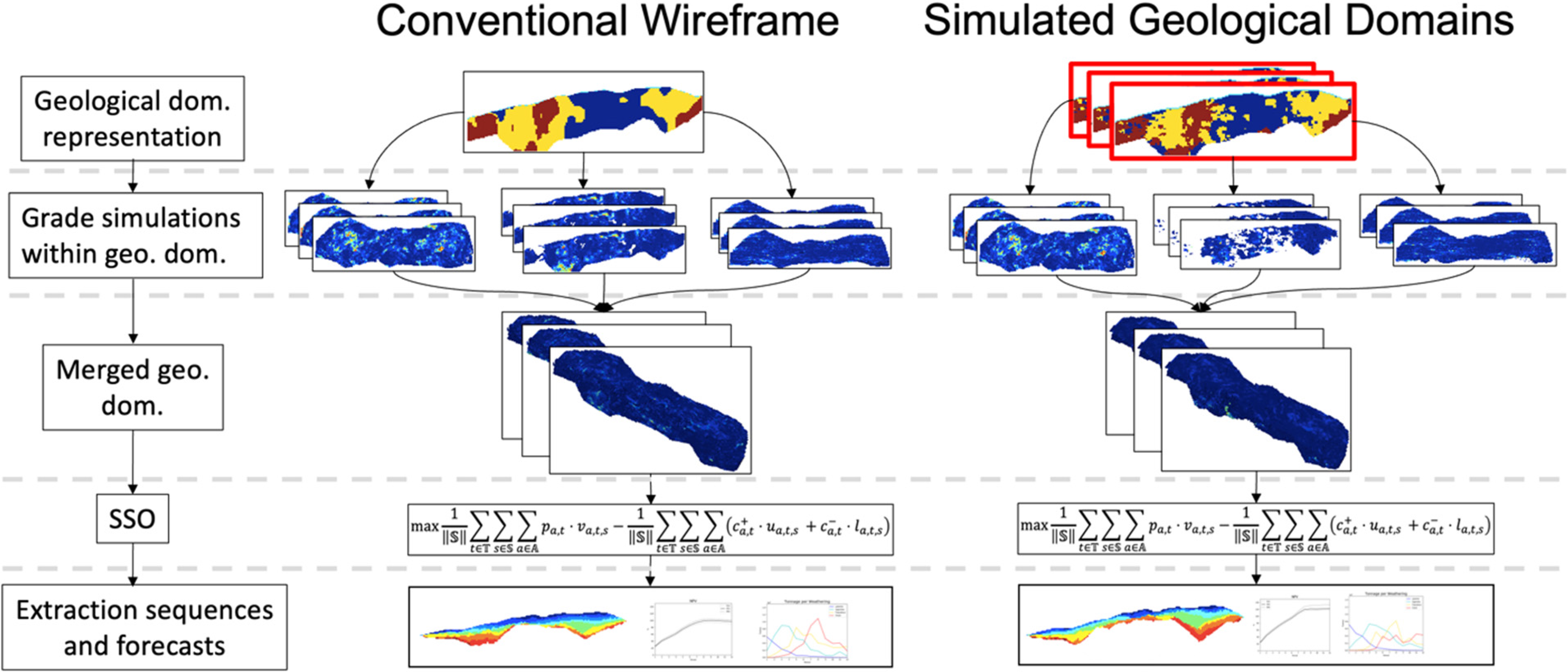
Workflows to compare the effects of high-order simulated geological domains. They start with the (a) representation of geological domains, respectively, (b) grades simulations, (c) merged geological domains into full orebody models, (d) SSO and (e) mine plans represented by extraction sequences and forecasts.

The following sections correspond to an overview of the categorical, continuous simulation methods, along with SSO. Next, the method's application to the Saramacca gold mine is described, and conclusions follow.

Methods

This section describes methods used to show the effects of the high-order simulation of geological domains in the stochastic LOM optimisation of mining complexes.

High-order simulation of geological domains

The high-order categorical simulation method used (Minniakhmetov and Dimitrakopoulos, 2022) did not require a training image. The main steps of the method are outlined as follows:

Having conditioning dataset, grid, and neighbourhood parameters:

Define random path visiting all the unsampled nodes from the grid.

For each node $x_{i_{0}}$ in the path without value assigned:

Find the closest data samples $x_{i_{1}}, x_{i_{2}}, \dots, x_{i_{n}}$ . The categories at these nodes are denoted by $k_{1}, \dots, k_{n}$ .

For all $k_{0} = 1 \dots K$ , calculate the high-order spatial indicator moments $M_{k} (Z_{i_{0}}, Z_{i_{1}}, \dots, Z_{i_{n}})$ .

Calculate conditional distribution from joint distribution

P (Z_{i_{0}} = k_{0} | Z_{i_{1}} = k_{1}, \dots, Z_{i_{n}} = k_{n}) = A M_{k} (Z_{i_{0}}, Z_{i_{1}}, \dots, Z_{i_{n}}),

(1)

where A is the normalisation coefficient

A = \frac{1}{\sum_{k_{o} = 1}^{K} M_{k} (Z_{i_{0}}, Z_{i_{1}}, \dots, Z_{i_{n}})} .

(2)

Draw a random value $z_{i_{0}}$ from conditional distribution and assign it to un-sampled location in the grid $x_{i_{0}}$

Add $z_{i_{0}}$ to the set of hard data sample and previously simulated values.

Repeat steps (a) to (e) for all the points in the path defined in step 1.

In summary, the method calculates conditional probability distribution functions from the joint distribution given by high-order spatial indicator moments.

DBSIM of grades

The DBSIM method of continuous attributes is detailed in Boucher and Dimitrakopoulos (2009), and can be considered as an extension of the generalised SGS method (GSGS) (Dimitrakopoulos and Luo, 2004). DBSIM overcomes the memory requirements and improves computational performance by considering block-support values as conditioning data, rather than only point-support values.

The main characteristic of the method is the inclusion of conditioning data from different support scales. Having conditioning dataset, discretisation and neighbourhood parameters, the main steps of the method are summarised as:

Perform normal-score transformation of conditioning data from data-scale to normal-score.

Define random path visiting each of the N blocks to be simulated.

For each block,

Generate simulated values of the internal nodes by considering conditioning normal-score data of both point and block supports, similar to LU simulation.

Average the simulated internal node to get a simulated block support in normal-score value.

Back-transform the internal normal-score values to get point support values in data-scale. Average these to get a simulated block support value in data scale.

Discard values of internal nodes and add the simulated block value in normal score to the conditioning data set; keep the block value in data scale as the result.

Repeat steps in (3), up until all the block N are simulated, for each of the realisation required.

Simultaneous stochastic optimisation of mining complexes

The simultaneous stochastic optimisation of mining complexes framework was presented and further described in Goodfellow and Dimitrakopoulos (2016, 2017). The framework models the mining complex as a network where material mass flows from sources to destinations, changing its value based on optimised decisions on when and where to send it. SSO maximises expected value while managing the risk of not meeting production targets and capacity constraints, such as mining, hauling, processing and stockpiling. Being based on the value of products rather than the economic value of blocks, allows the simultaneous incorporation of non-linear relations such as blending and recoveries. The outputs of SSO correspond to a feasible and optimised production schedule, along with technical and financial forecasts.

The mining complex $C$ may be composed of several sources of material, such as mines or other external sources $M$ , stockpiles $S$ , processors $P$ and a waste dump $W$ . Material from the mines is discretised in selective mining units (also known as mining blocks) $b \in B_{m}$ , where $B_{m}$ represents the set of blocks in a mine m. Blocks are modelled with primary and secondary attributes. Primary attributes $p \in P$ , such as valuable material's mass, are sent from one location to another in an additive manner. Hereditary attributes $h \in H$ , such as chemistry, recovery or economic value, are calculated as functions of primary attributes at each location. Specifically, hereditary attributes enable the inclusion of non-linearities into the mathematical programming model. For each location $i \in M \cup S \cup P \cup W$ in the mining complex, materials and their attributes can be sent and received from a distinct set of locations, $I (i)$ and $O (i)$ , respectively. Geological uncertainty is considered by simulating categorical and continuous attributes for each block, each scenario $s \in S$ has equal probability of occurring.

There are three types of decision variables: extraction sequence, destination policy and processing stream. A binary decision variable $x_{b, t} \in {0, 1}$ determines the extraction sequence of a mine and is equal to one if block b is mined in period t and zero otherwise. A block b is available for extraction if its predecessors in set $O (b)$ are extracted at the same period $t \in T$ or before. Predecessor are calculated in a pre-processing step. A binary decision variable $z_{g, j, t}$ determines the destination policy a group $g \in G$ of material that is sent to a destination $j \in O (g)$ in each period t. Groups are generated in a pre-processing step using k-means + + clustering algorithm to define the boundaries of the groups. Blocks may be sent to different destinations across various scenarios but are optimised using a scenario independent destination policy that assigns membership to the group g for each block b in scenario s. The continuous variables $y_{i, j, t, s}$ ∈ [0,1] determines the proportion of material sent from stockpile $i \in S$ to location $j \in P$ in period $t \in T$ and scenario $s \in S$ . Lastly, the value of a primary or hereditary attribute is denoted as $v_{p, i, t, s}$ and $v_{h, i, t, s}$ , respectively, for each location $i \in S \cup P$ in period $t \in T$ , and scenario $s \in S$ .

Revenues and expenditures are incurred throughout the mining complex, which are modelled as hereditary attributes and are directly incorporated into the objective function by calculating a discounted value $p_{h, i, t} = \frac{p_{h, i, 1}}{{(1 + d)}^{t}}$ where d is the economical discount rate utilised. Costs can be separated into mining, hauling, rehandling, processing and waste categories for each hereditary attribute h, at location i and period t. Lower (-) and upper (+) deviation variables $d_{h, i, t, s}^{-}$ and $d_{h, i, t, s}^{+}$ are introduced along with their respective penalty costs $c_{h, i, t}^{-}$ and $c_{h, i, t}^{+}$ for managing deviations from production targets or capacities. A geological discount rate $d_{g e o}$ is also applied to deviation costs to defer riskier material to later periods, $c_{h, i, t} = \frac{c_{h, i, 1}}{{(1 + d_{g e o})}^{t}}$ .

\begin{aligned} max \frac{1}{| S |} \sum_{s \in S} \sum_{t \in T} & {\underset{P a r t I}{\underset{⏟}{\sum_{i \in P} \sum_{h \in H} p_{h, i, t} \cdot v_{h, i, t, s}}} - \underset{P a r t I I}{\underset{⏟}{\sum_{i \in M \cup S \cup P} \sum_{h \in H} (c_{h, i, t}^{-} \cdot d_{h, i, t, s}^{-} + c_{h, i, t}^{+} \cdot d_{h, i, t, s}^{+}}})} \\ - \underset{P a r t I I I}{\underset{⏟}{\sum_{t \in T} \sum_{b \in W_{b}} \sum_{i \in M} (c_{b, t, i}^{s m o o t h} \cdot d_{b, t, i}^{s m o o t h}) - \sum_{t \in T} \sum_{b \in V_{b}} \sum_{i \in M} (c_{b, t, i}^{s i n k} \cdot d_{b, t, i}^{s i n k})}} \end{aligned}

(3)

The objective function (Equation (3)) of the mathematical model maximises the net present value (NPV) that is generated by producing a set of marketable materials and minimises the risk of failing to meet production targets and environmental requirements. Part I maximises the profits generated from selling products. Part II minimise the deviations from mining, hauling, stockpiling and processing capacities. Part III corresponds to mineability constraints.

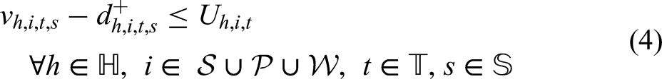
The mining, hauling, stockpiling and processing capacity constraints are managed to satisfy the operational capabilities of the mine by calculating the deviations $d_{h, i, t, s}^{+}$ and $d_{h, i, t, s}^{-}$ from the upper $U_{h, i, t}$ , and lower $L_{h, i, t}$ limits, respectively, and penalising the deviations through discounted costs $c_{h, i, t}^{+}$ and $c_{h, i, t}^{-}$ in the objective function ( $P a r t I I$ ). Mining and hauling capacities are determined by the equipment required to those activities. Stockpiles are bounded by the available space in the run-of-mine stockpiling facility. Processing capacity is determined by plant processing constraints, and particularly the mill capacity. Capacity constraints are demonstrated as follows

v_{h, i, t, s} - d_{h, i, t, s}^{+} \leq U_{h, i, t} \forall h \in H, i \in S \cup P \cup W, t \in T, s \in S

(4)

v_{h, i, t, s} + d_{h, i, t, s}^{-} \geq L_{h, i, t} \forall h \in H, i \in S \cup P \cup W, t \in T, s \in S .

(5)

A destination policy constraint also ensures that a group can only be sent to one destination within the mining complex:

\sum_{j \in O (g)} z_{g, j, t} = 1 \forall g \in G, t \in T

(6)

Mineability constraints are also considered to ensure feasibility of the extraction sequence. Blocks within a horizontal window around block b and blocks above it, in a certain pit i become members of a set

W_{b, i}

and

V_{b, i}

, respectively. The quantity of blocks in

W_{b, i}

and

V_{b, i}

mined in different periods than block b becomes

d_{b, t, i}^{s m o o t h}

and

c_{b, t, i}^{s i n k}

, respectively, associated with discounted penalty costs

c_{b, t, i}^{s m o o t h}

and

c_{b, t, i}^{s i n k}

Producing a schedule for mining is difficult in a complex mining environment because of the numerous factors that need to be optimised at the same time. Most commercial optimisation tools simplify the issue by using a single estimated model, but this overlooks the unpredictability of orebody models. The probabilistic approaches used in this study make the optimisation more challenging, necessitating the use of a heuristic method to find solutions. Goodfellow and Dimitrakopoulos (2016, 2017), Lamghari et al. (2014) and Lamghari and Dimitrakopoulos (2020) explain various heuristic techniques. In this work, a combination of multi-neighbourhood simulated annealing with adaptive neighbourhood search is used (Goodfellow and Dimitrakopoulos, 2016, 2017). The method employed necessitates an initial viable solution, which is derived using a greedy algorithm designed to optimise the objective function while adhering to slope constraints. This preliminary solution undergoes various perturbations to yield an alternative solution. If this new outcome is superior, the related decision variables are incorporated. Conversely, if the solution does not improve, it may still be considered, but with a progressively diminishing likelihood.

Application: Case study at the Saramacca gold deposit

The Saramacca gold deposit is located approximately 25 km southwest of the Rosebel Gold Mine milling facility and was owned by IAMGOLD Corp. at the time of the study. This facility is located approximately 80 km south of the city of Paramaribo, capital of Suriname.

Stochastic simulation of the Saramacca gold deposit

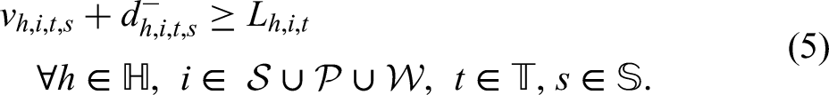
The wireframe representation of lithologies (geological domains) of the Saramacca gold deposit is shown in Figure 2. The lithologies simulated correspond to the following three domains: fault zone, pillow basalt and rest. Laterite was considered as a thin (<10 m) sedimentary top layer, not simulated. Drillholes with pyroclastic information were not considered. The Fault Zone corresponds to a vertical zone which is associated with rich gold mineralisation, as shown in Figure 4(b). The rest zone corresponds to a barren lithology that encompasses Massive Basalt and Amygdular Basalt, both combined given their similar properties and considered to limit the SW extent of the gold-rich fault zone (Payeur et al., 2018).

Figure 2.

Plan view of Saramacca Gold deposit lithologies (Payeur et al., 2018).

Figure 4.

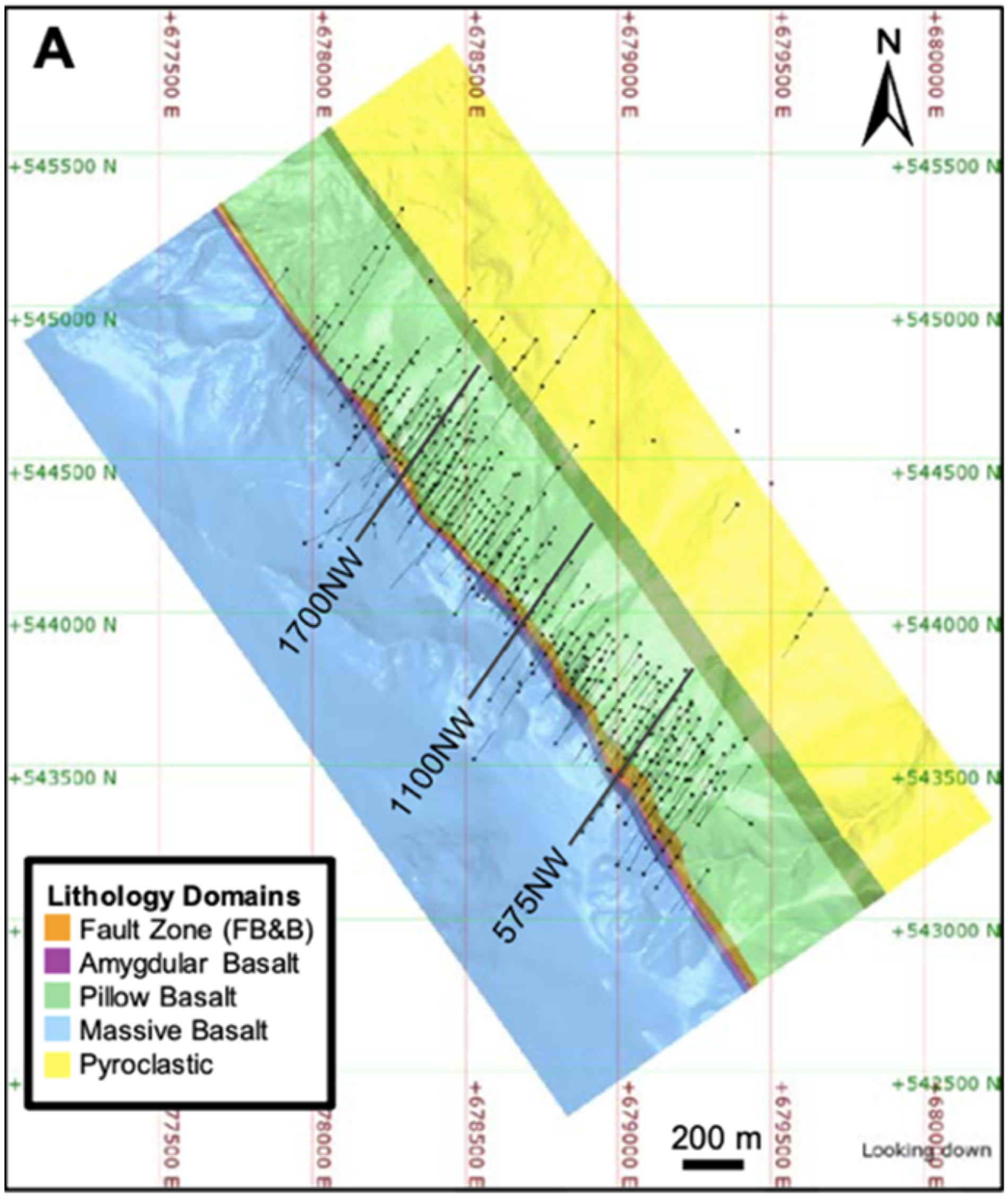
Histograms for mineralised lithologies (a) laterite, (b) fault and (c) pillow basalt.

Available data includes 473 exploration drillholes spaced about 50–60 m and composited in 5 m heights. North in Figure 3(a) is rotated 55 deg. counterclockwise with respect to north in Figure 2. Sampled dimensions in volume in Figure 3 are about 2 × 1 × 0.5 km in east-west, north-south, and up-down directions, respectively.

Figure 3.

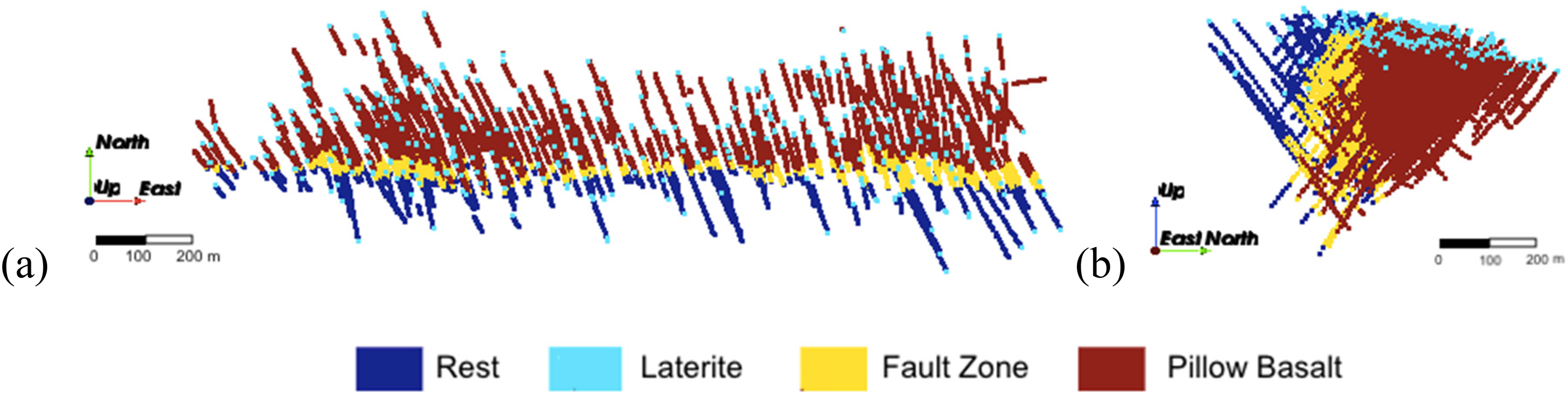
Top (a) and lateral (b) views of exploration drillholes. Light blue, yellow and red corresponds to Laterite, Fault and Pillow Basalt respectively. Dark blue corresponds to other lithologies combined of no interest named rest. Fault zone, pillow basalt and rest were simulated while laterite was considered deterministic.

Gold grade histograms based on drillhole data for the three mineralised domains simulated are found in Figure 4.

The mineral deposit is also modelled through different deterministic weathered types of materials shown in Figure 5. The weathered rock types are not simulated, and they were used as provided (Payeur et al., 2018), as they are related to different geotechnical and metallurgical parameters, along with drilling, blasting and processing costs. Deeper in the mineral deposit, the rock is more competent and less weathered for which costs and slope angles increase while recovery decreases (Payeur et al., 2018). The rock types are typically sorted along the vertical direction, starting at the top with the most weathered (less competent) thin layer of laterite and saprolite, to the less weathered (more competent) thick layers of transition and fresh rock.

Figure 5.

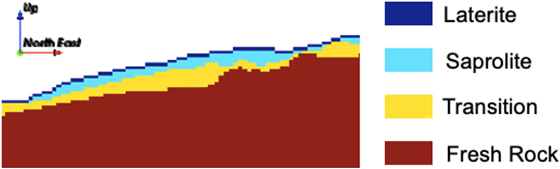
Vertical section of deterministic weathering profiles (not simulated).

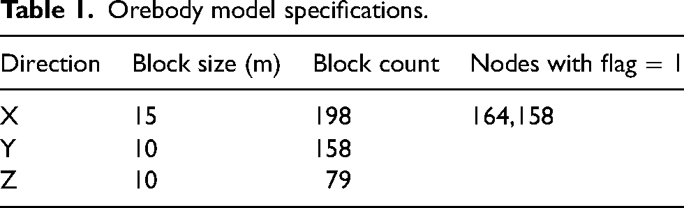
Orebody model specifications are found in Table 1. To account for the topography and mineralised volume, an arbitrary and deterministic flag was defined as 1 to each of the nodes to be assigned with a geological domain value (active for computation) and −999 for the rest (non-active for computation). The set of flagged nodes is named mask, and sections of it are shown in Figure 6. Positive flagged nodes outline the mineralisation and determine the domain where the categorical simulations of the geological domain will be generated. The use of a mask allows the simulation to be constrained by the topography and reduces the computational time as not all the nodes in a parallelepiped are needed to be computed (Mariethoz and Caers, 2015).

Figure 6.

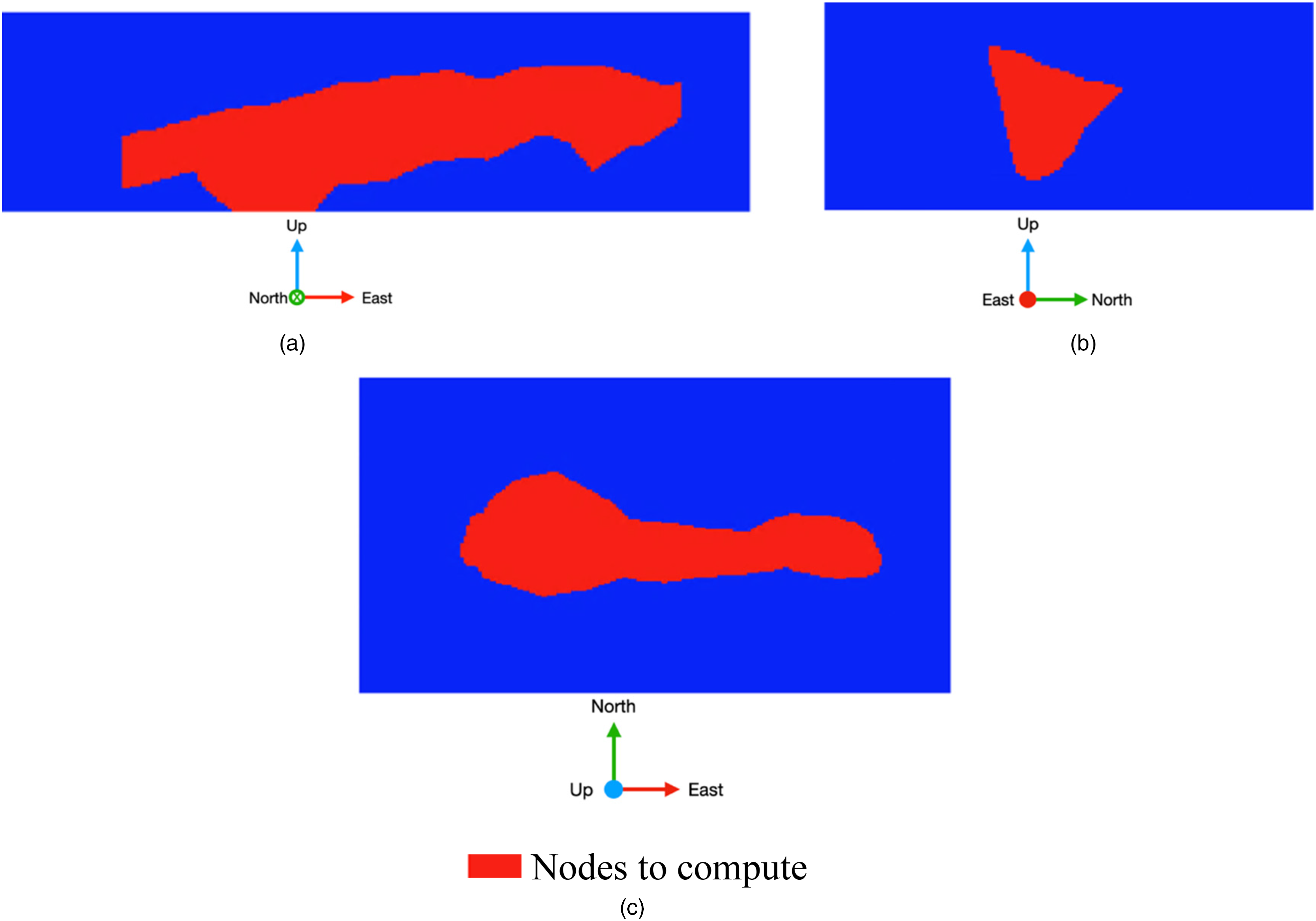
Sections of computational mask. Vertical (a), (b) and horizontal (c). Red and blue indicate nodes to compute and not compute, respectively.

Table 1.

Orebody model specifications.

Direction	Block size (m)	Block count	Nodes with flag = 1
X	15	198	164,158
Y	10	158
Z	10	79

Two sections of the given wireframes and two sections for each of the two categorical simulations of the geological domains (lithologies) are shown in Figure 7. Fifteen realisations were used, because it has been documented that 10–15 simulations are sufficient to generate stable results in long-term mine planning and production scheduling (Albor and Dimitrakopoulos, 2009; Montiel and Dimitrakopoulos, 2017). Given wireframes present smoother boundaries between the geological domains than realisations, that rather show high variability in these boundaries while maintaining consistency with data in the location of the domains. This local variability is a consequence of the uncertainty inherent in the sparse data sampled.

Figure 7.

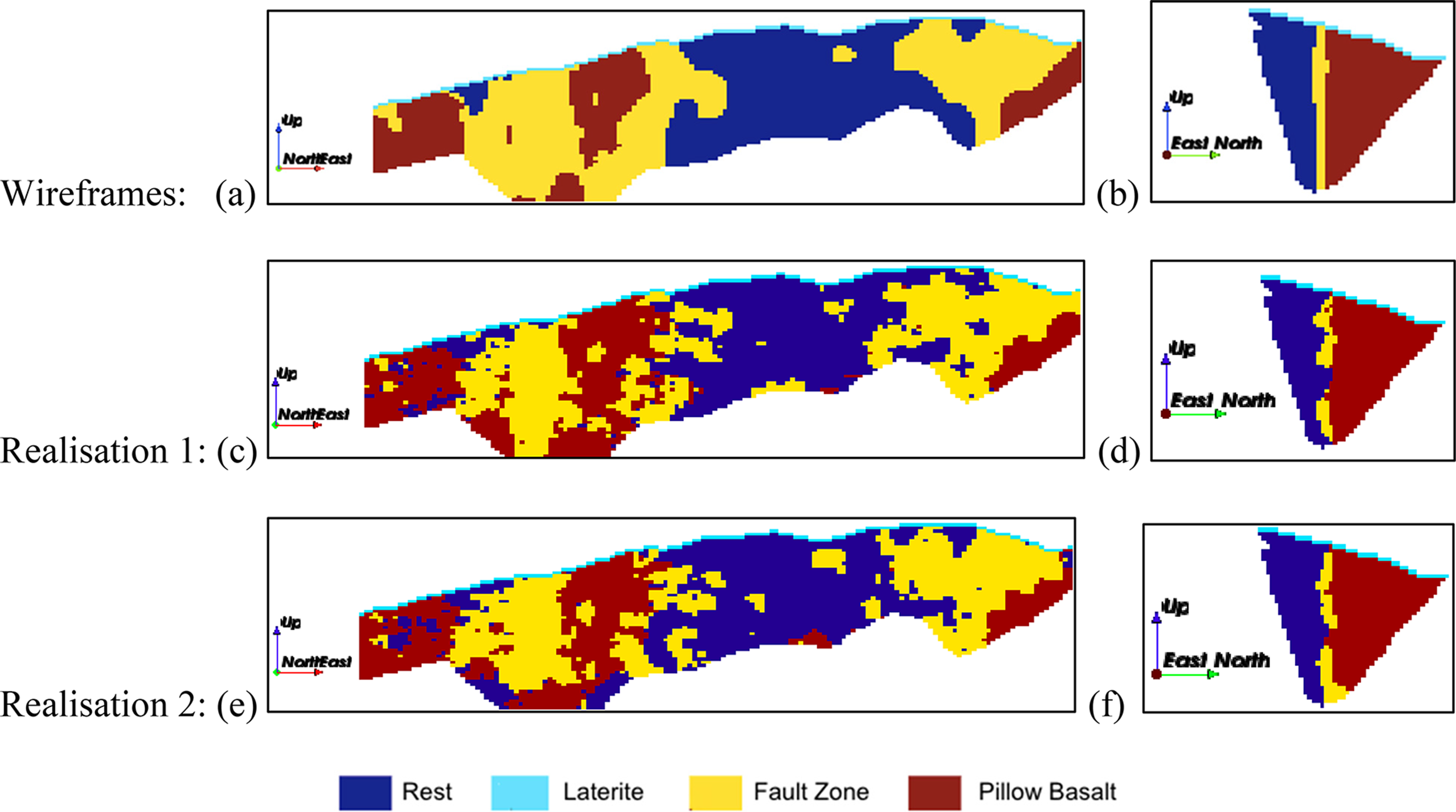
Vertical sections of geological units by given wireframes (a), (b); and two randomly selected realisations of simulated geological units (c)–(f).

The local variability of boundaries is more evident in the realisations than in the given wireframes, as shown in Figure 7(a) and (b). For the fault zone, in particular, which is the geological domain related with the highest grades, the more variable representation of boundaries in the realisations could render a different extraction sequence rather than using the single continuous and smoothed interpretation given by the wireframes.

The statistics considered for validation correspond to their respective orders. The first-order statistic corresponds to the probability of a single block to belong into a certain geological unit (one-point statistic), that is, the proportions of each geological unit in the domain of computation. Second-order corresponds to the traditional indicator variogram along certain directions, which is related to the joint probability of two points along one dimension to have the same values. Third and higher orders are given by the joint probability of corresponding points to belong to certain geological units. Joint probabilities are given by high-order spatial indicator moments. In this case, validation is shown up until the fourth order. For the following comparison of statistics, it must be noted that, rather than an exact collation, validation is done by considering the reproduction of main patterns.

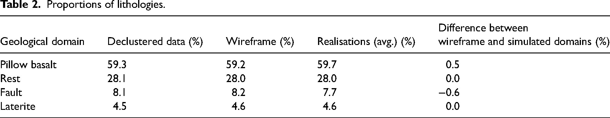
As seen in Figure 8 and in Table 2, declustered proportions of each geological unit for the wireframed and realisation sets are similar; it is expected that the results are driven by the spatial distribution of these geological units rather than by their proportions. The biggest proportion corresponds to Pillow Basalt followed by rest, fault and laterite.

Figure 8.

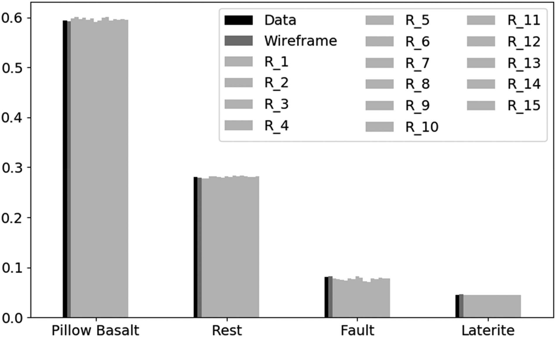
Proportions of lithologies given wireframed and simulated geological units.

Table 2.

Proportions of lithologies.

Geological domain	Declustered data (%)	Wireframe (%)	Realisations (avg.) (%)	Difference between wireframe and simulated domains (%)
Pillow basalt	59.3	59.2	59.7	0.5
Rest	28.1	28.0	28.0	0.0
Fault	8.1	8.2	7.7	−0.6
Laterite	4.5	4.6	4.6	0.0

Table 3.

Mining complex parameters.

Mine	Hauling	Stockpiles	Processor	General
Drilling and blasting costs^a	Hauling cost	Rehandling cost	Recovery^a	Economic discount rate
Mining cost	Hauling capacity		Processing cost^a	Geological discount rate
Closure costs			Processing capacity	Gold price
Dumping costs				Selling costs
Mining capacity				Royalties
Mineability parameters^b				Fixed costs
				Optimisation parameters^b

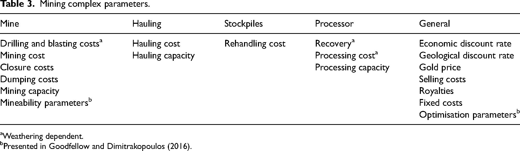
^aWeathering dependent.

^bPresented in Goodfellow and Dimitrakopoulos (2016).

Indicator variograms are calculated and shown in Figures 9–12, for each mineralised geological unit along the different directions, for the data, and the realisations. More detail on wireframed information can be found in the corresponding NI 43-101 report (Payeur et al., 2018). In general, data variability is reproduced. Laterite presents less variability than fault and basalt geological units for the lags shown. High reproduction of variability of basalt is attributed to the fact that it is the geological unit with the highest quantity of samples.

Figure 9.

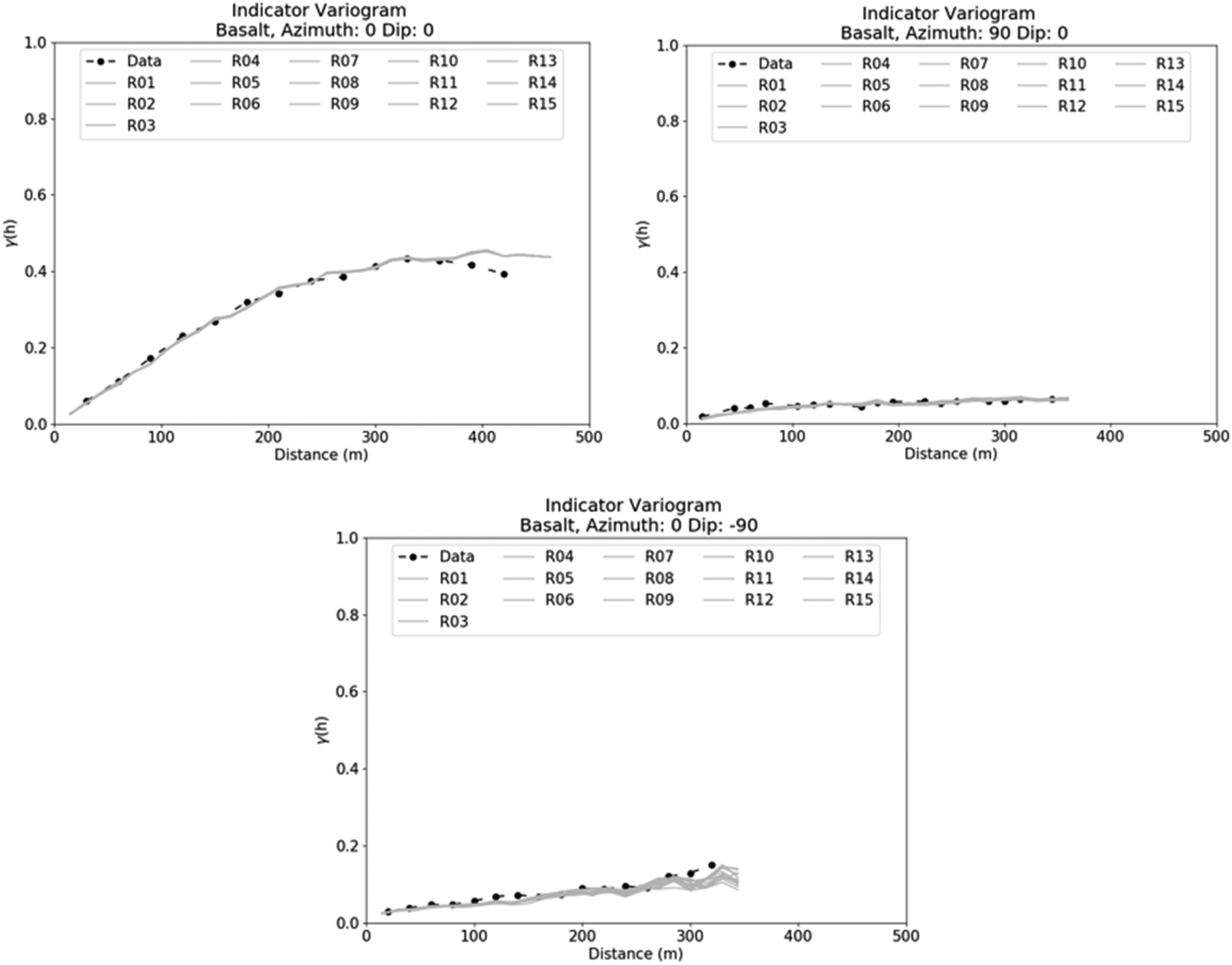
Indicator variograms of pillow basalt for different directions.

Figure 10.

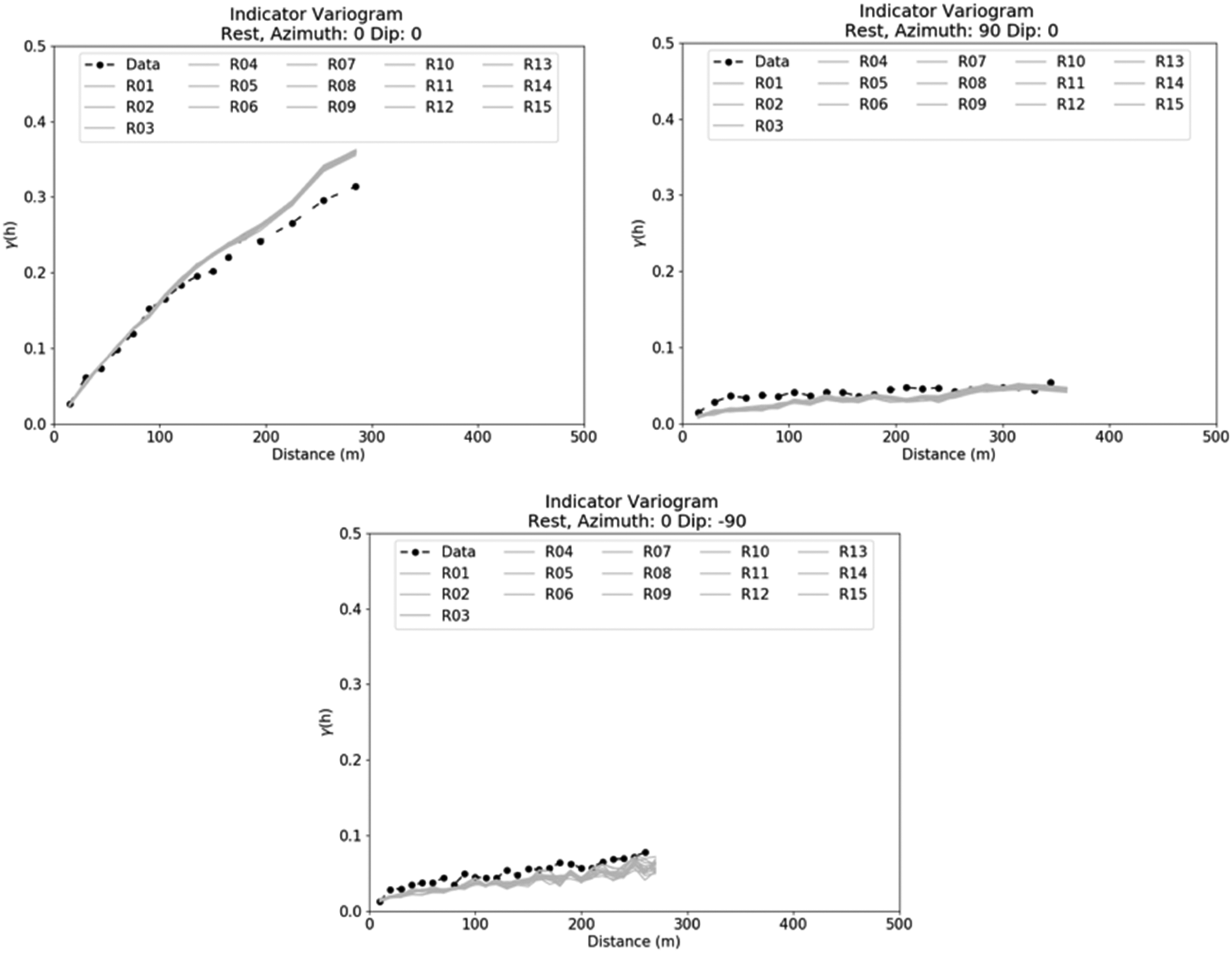
Indicator variograms of rest for different directions.

Figure 11.

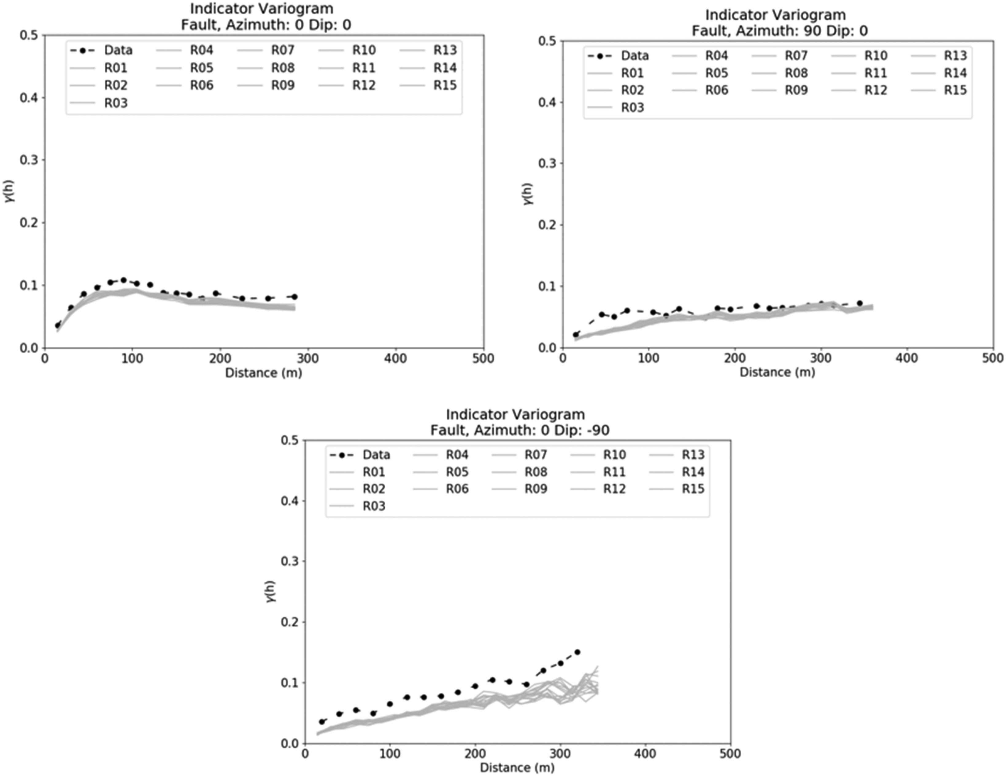
Indicator variograms of fault for different directions.

Figure 12.

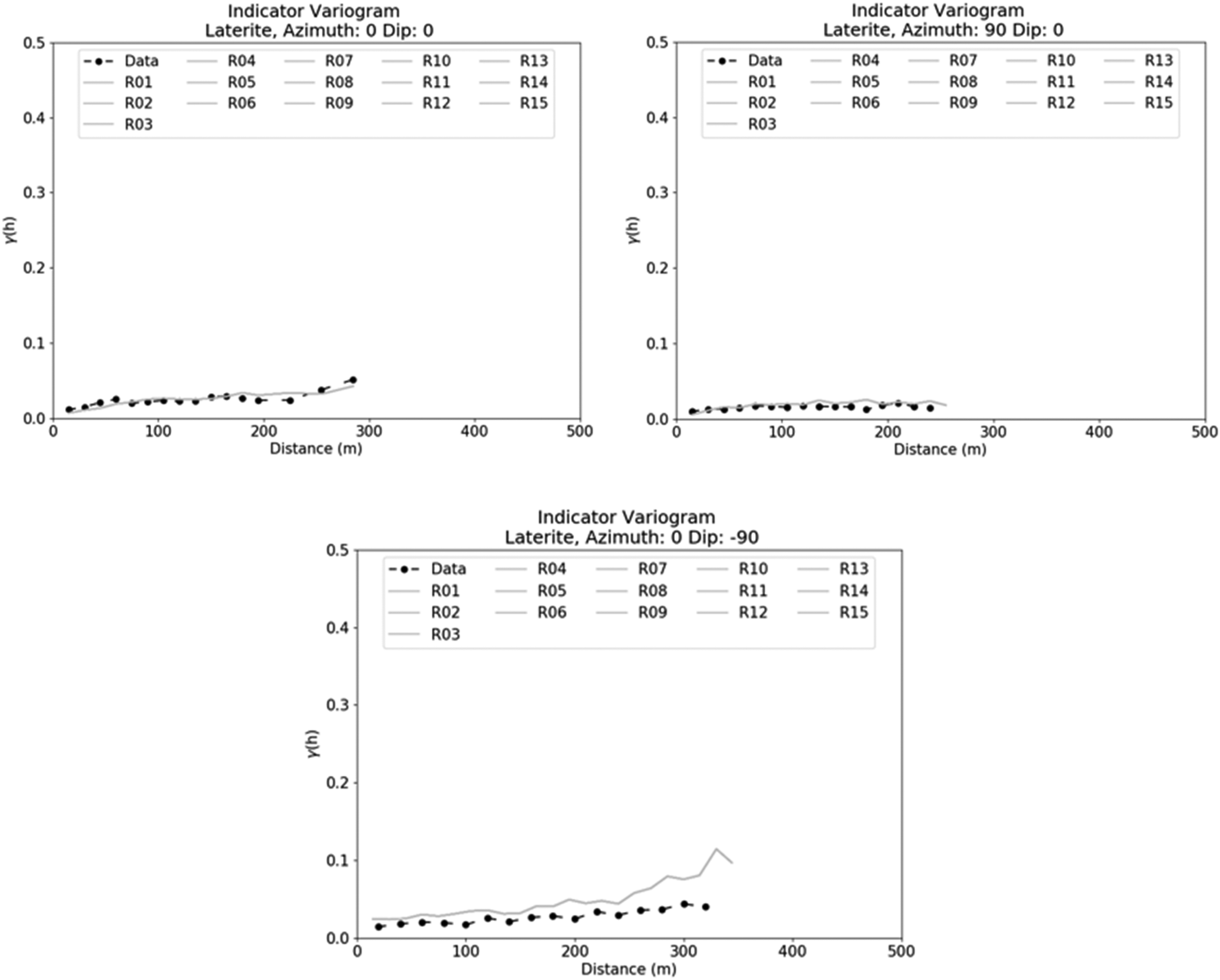
Indicator variograms of laterite for different directions.

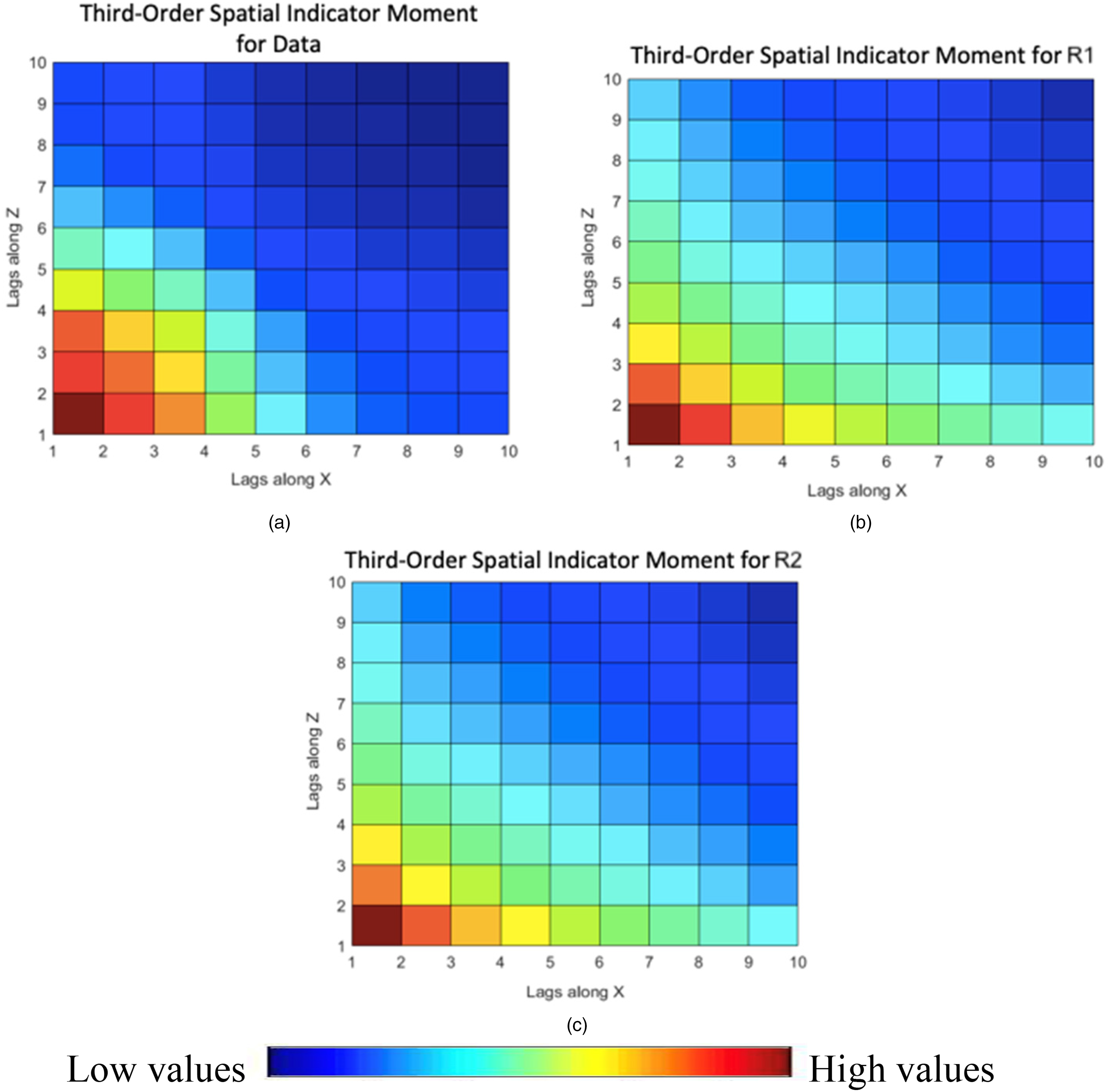
The validation of higher-order statistics is done through the reproduction of the joint-probability distributions of having certain categories at respective positions, in an orthogonal template, represented by high-order spatial indicator moments maps. The codification of {Rest:0; Laterite:1; Fault:2; Basalt:3} is used for the indexation of $\hat{M}$ . Figure 13 shows the third order spatial indicator moment map for fault geological domain for two directions of an L-shape template, for different lags, noted as ${\hat{M}}_{222} (h_{1}, h_{2})$ , with lags $h_{1} = (i d x, 0, 0)$ and $h_{2} = (0, 0, k d z)$ , indexed by $i, k = 1, \dots, 10$ where $d x$ and $d z$ are 15 m × 10 m, respectively. As expected, the joint probability is higher for shorter lags, shown in red, rather than long ones, shown in blue, meaning that there is a higher chance of finding this pattern of geological unit in shorter, rather than longer, distances. It is also found that this relation is similar for vertical (Z) and horizontal direction (X), not showing any preferential behaviour for one of these directions.

Figure 13.

Third-order spatial indicator moment maps ${\hat{M}}_{222} (h_{1}, h_{2})$ . Approximated spatial indicator moment of data (a) and of two realisations (b) and (c).

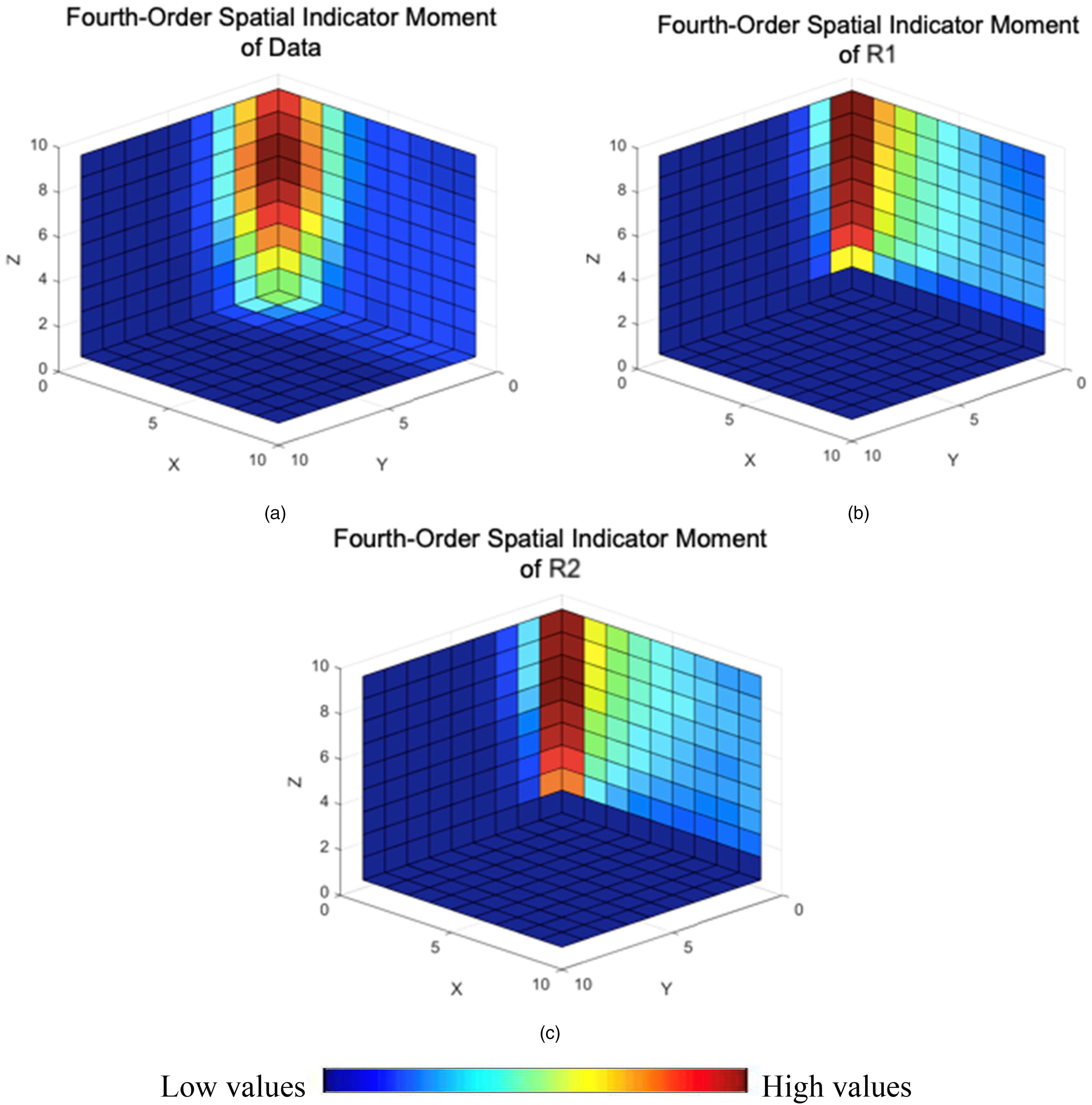
Finally, Figure 14 shows the fourth-order spatial indicator moments where the centre and horizontal values in X and Y directions correspond to fault zone, while the last vertical Z correspond to basalt, noted ${\hat{M}}_{2223} (h_{1}, h_{2}, h_{3})$ , with lags $h_{1} = (i d x, 0, 0)$ , $h_{2} = (0, j d y, 0)$ and $h_{3} = (0, 0, k d z)$ , indexed by $i, j, k = 1, \dots, 10$ , where $d x$ , $d y,$ and $d z$ are 15 m × 10 m × 10 m. As fault zone is a relatively thin zone with respect to the Y (S-N) direction, low probabilities are found for almost any lag higher than two in this direction. It is also noted that, as the statistic’s order increases, comparing data with realisations becomes more difficult. This is because the former has fewer repetitions than the latter.

Figure 14.

Fourth-order spatial indicator moment for fault zone in vertical, strike and perpendicular to strike directions noted ${\hat{M}}_{2223} (h_{1}, h_{2}, h_{3})$ . Approximated spatial indicator moment of data (a) and of two realisations (b) and (c).

The simulation and validation of gold grades are performed for each mineralised geological domain by using the DBSIM method. Two sets of geological scenarios are defined. The first set considered the simulation of grades inside wireframed geological domains shown in Figure 7(a) and (b). The second set considered the full geological uncertainty given by the simulated geological domains and gold grades within them.

The data available for each mineralised geological domain corresponds to the capped exploration drillholes from 2018, composited in 5 m (Payeur et al., 2018). It is noted that the richest mineralised zone corresponds to the fault zone, which is also characterised with the highest gold grade variance. The laterite domain follows with lower average grades; however, as seen in Figure 7, it only represents a thin top layer of no more than 10 m of depth (Payeur et al., 2018). Finally, the pillow basalt domain presents the lowest average gold grade, but corresponds to the lithology with the most data records and relatively low variance.

Gold grade realisations for both sets, wireframed and simulated geological domains, are shown in Figure 15. The main difference between gold grade realisations within wireframed and simulated geological domains is the domain's spatial variability. This is particularly seen in fault zone, Figure 15(c) and (d), where the simulated domain in Figure 15(d) presents higher local variability than the wireframed domain in Figure 15(c). The clustered representation shown in Figure 7(d) and (f) allows high grades to be connected within clusters, rather than the thin vertical continuous domain shown in Figure 7(b).

Figure 15.

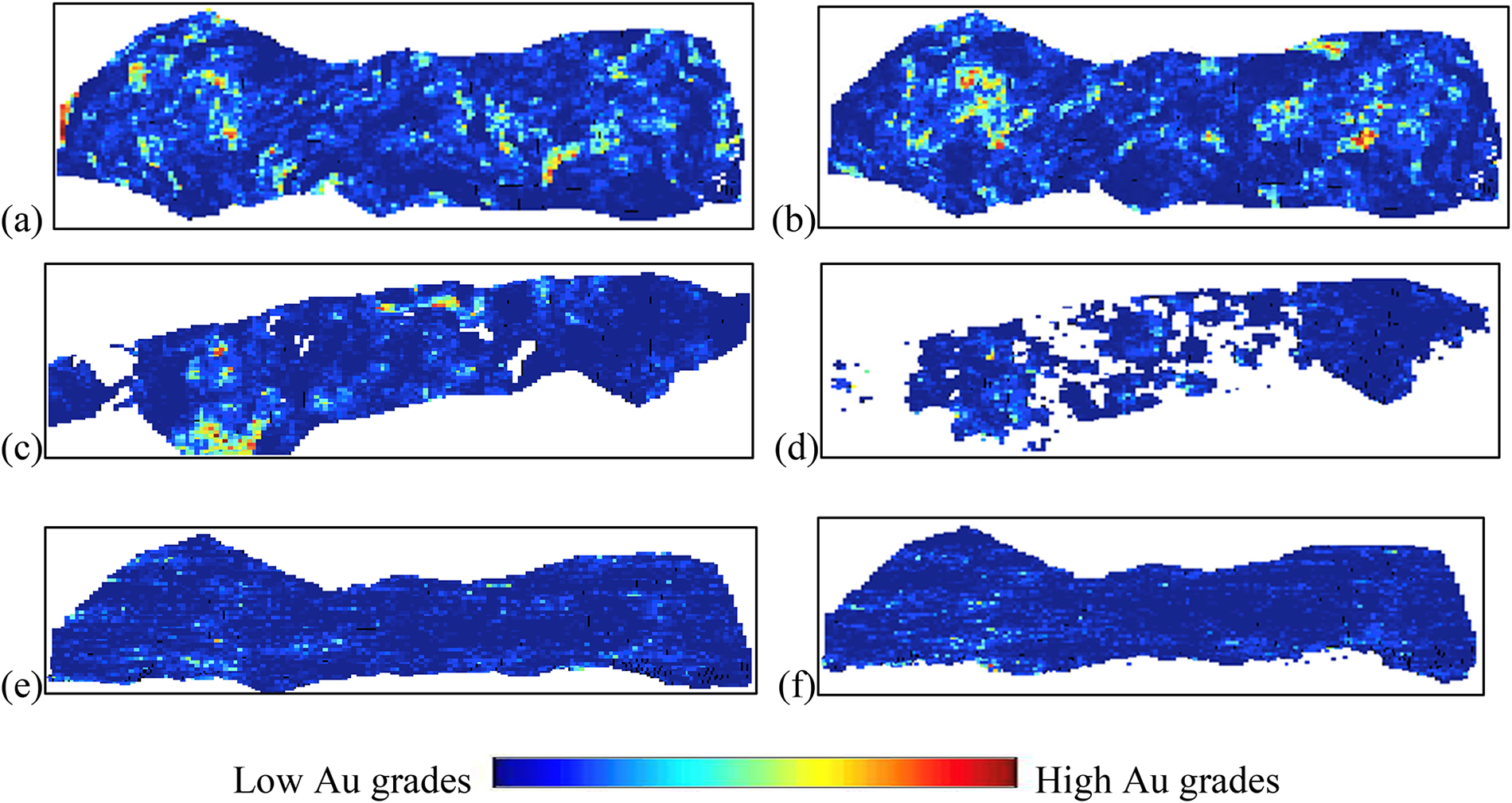
Top view of grade realisations within laterite within wireframed and simulated geological domains (a) and (b). Vertical view of grade realisations within fault zone within wireframed and simulated geological domains (c) and (d). Top view of grade realisations within basalt within wireframed and simulated geological domains (e) and (f).

E-types in Figure 16(a) highlight one artefact of using a deterministic representation of geological units, as a high-grade zone is drastically discontinued by a barren domain, while simulated domains in Figure 16(b) consider the possible mineralisation in that area. This will later translate into different extraction sequences, where the schedule based on the wireframed domains considers more waste to handle than the one based on simulated domains, thus increasing the costs and reducing the profit at the related financial forecasts.

Figure 16.

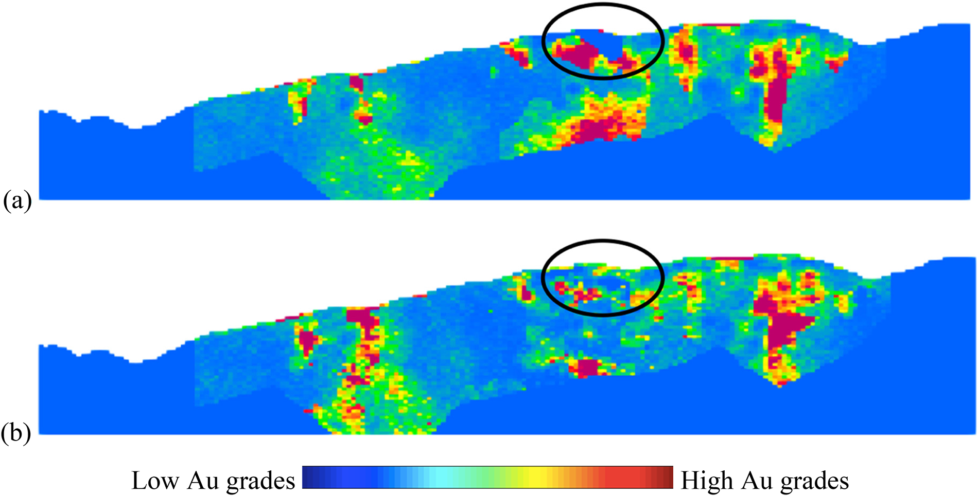
Vertical sections of e-types for (a) wireframed and (b) simulated geological domains. Black oval highlight differences.

Figure 17.

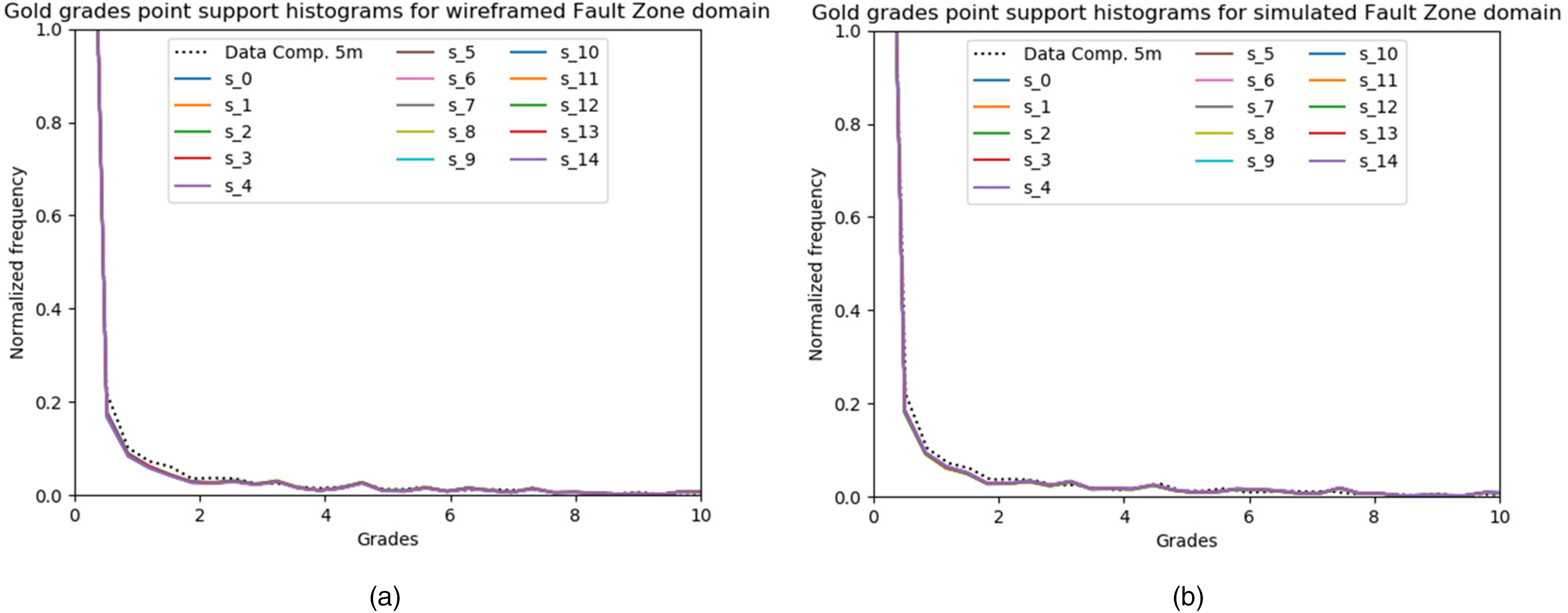
Histograms of gold grades within fault zone for (a) wireframed, and (b) simulated geological domains.

Figure 18.

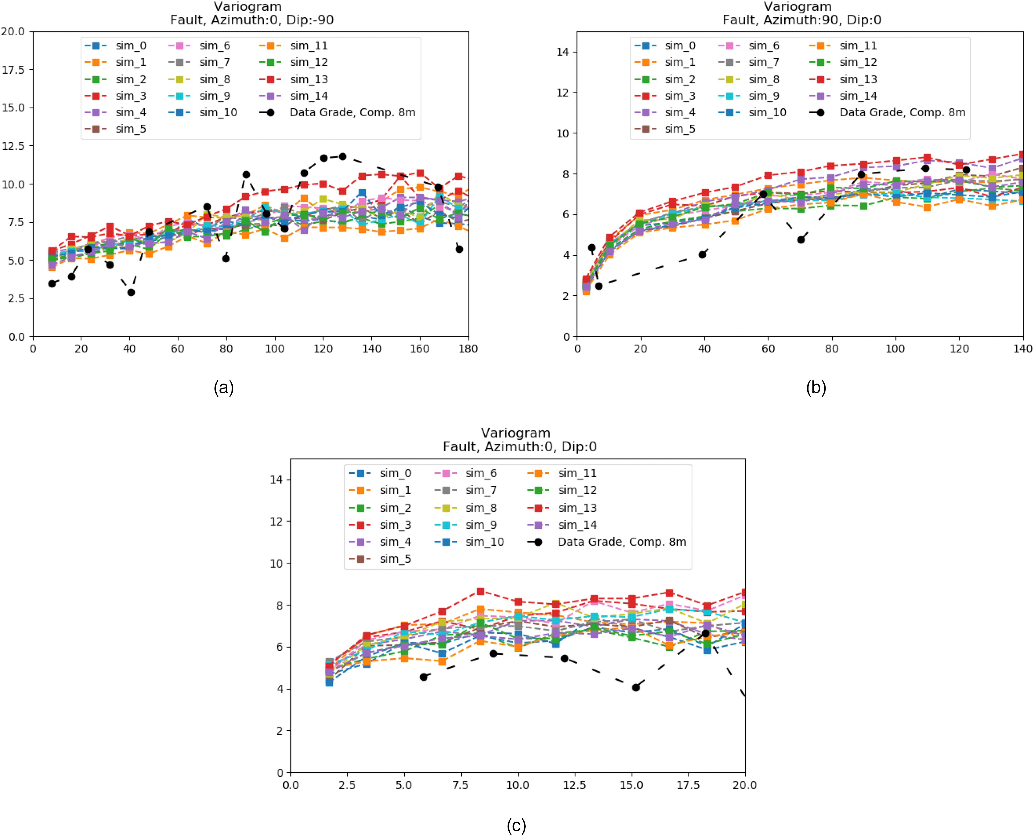
Variograms for gold grades in fault zone for simulated geological domains.

Validation of grade simulations is done by comparing first- and second-order statistics (histogram and variograms) of sample data and realisations in Figures 17 and 18, respectively, for simulated geological domains.

Simultaneous stochastic optimisation of the mining complex

The simultaneous stochastic optimisation framework is applied to the gold mining complex schematised in Figure 19. This study aims to explore how simulated lithologies of a gold deposit impact the strategic mine plan. The complex includes one open pit mine, an adjacent waste dump, and two stockpiles situated close to a processing mill. The two stockpiles are designated for soft and hard rocks; with the soft stockpile containing laterite and saprolite, while the hard stockpile holds transition and fresh rock types.

Figure 19.

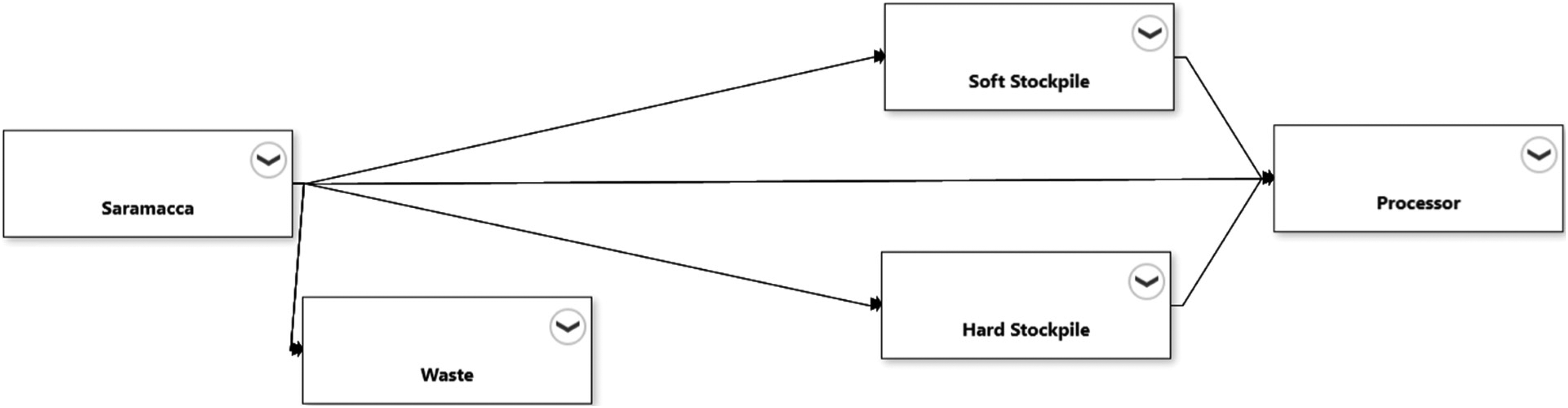
Mining complex modelled.

All extracted material that is not economically profitable to process is sent to the nearby waste dump. This destination policy is simultaneously optimised and does not require the input of pre-defined cut-off grades; rather, it comes out as an output of the optimisation process. Profitable material is hauled to stockpiles and a processor, constrained by the capacity of the truck fleet. Material is reclaimed from the stockpiles with generic equipment for which no capacity constraint is considered.

A summary of parameters considered in the optimisation is shown in Table 3.

Long-term production mine schedules for both sets, wireframed and simulated geological domains, are shown in Figure 20(a) and (b), respectively. As highlighted in Figure 20, extraction sequences are different for the two sets of simulations. These differences are attributed to the different spatial distributions of geological domains given by wireframes and simulated geological domains. As extraction sequences are different, ultimate-pit limits are also different. It must be noted that mineability constraints and parameters are the same for both optimisations, for which they have no influence in different extraction sequences. Economic and production forecast for schedules based on both sets, wireframed and simulated geological domains, are shown in Figures 21–27.

Figure 20.

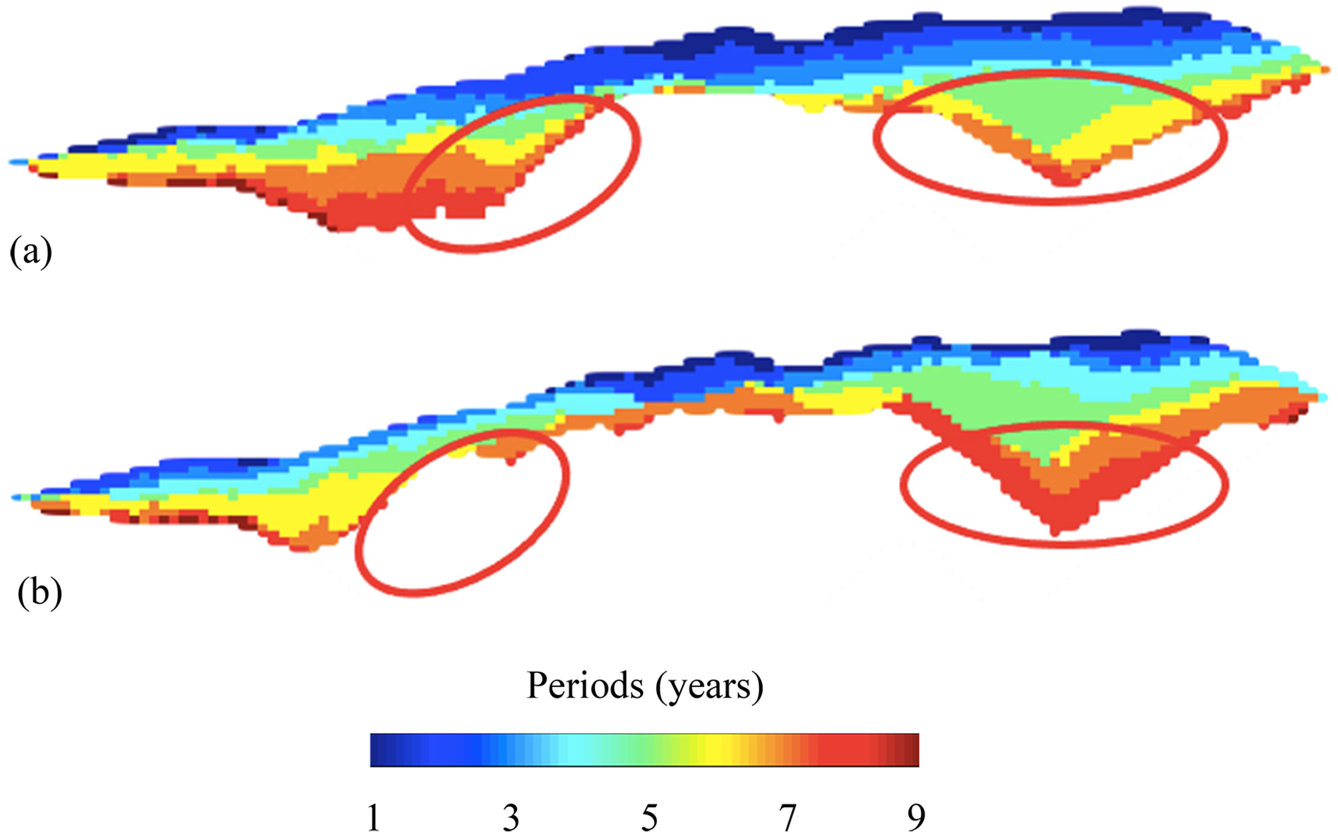
Vertical sections of extraction sequences for (a) wireframed and (b) simulated geological domains. Red ovals highlight differences.

Figure 21.

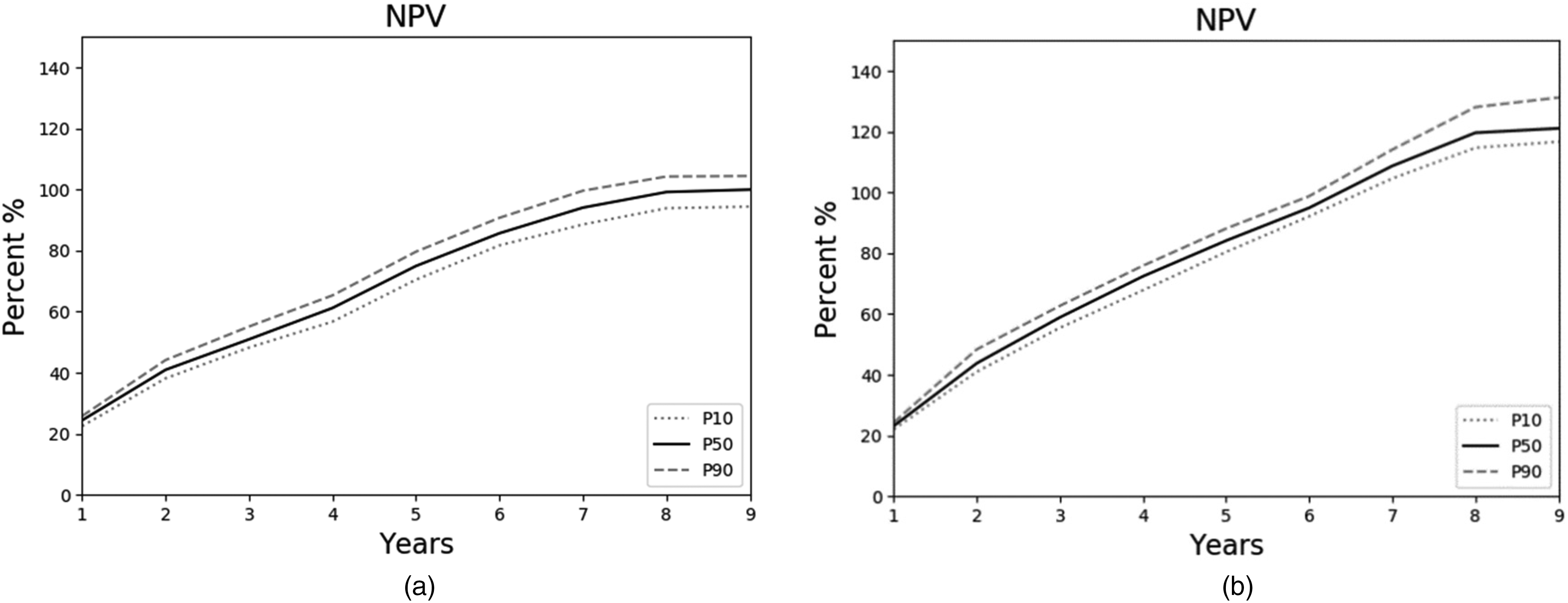
Scaled net present value (NPV) forecasts from schedules obtained from (a) wireframed and (b) simulated geological domains. Values scaled using year nine in (a).

Figure 22.

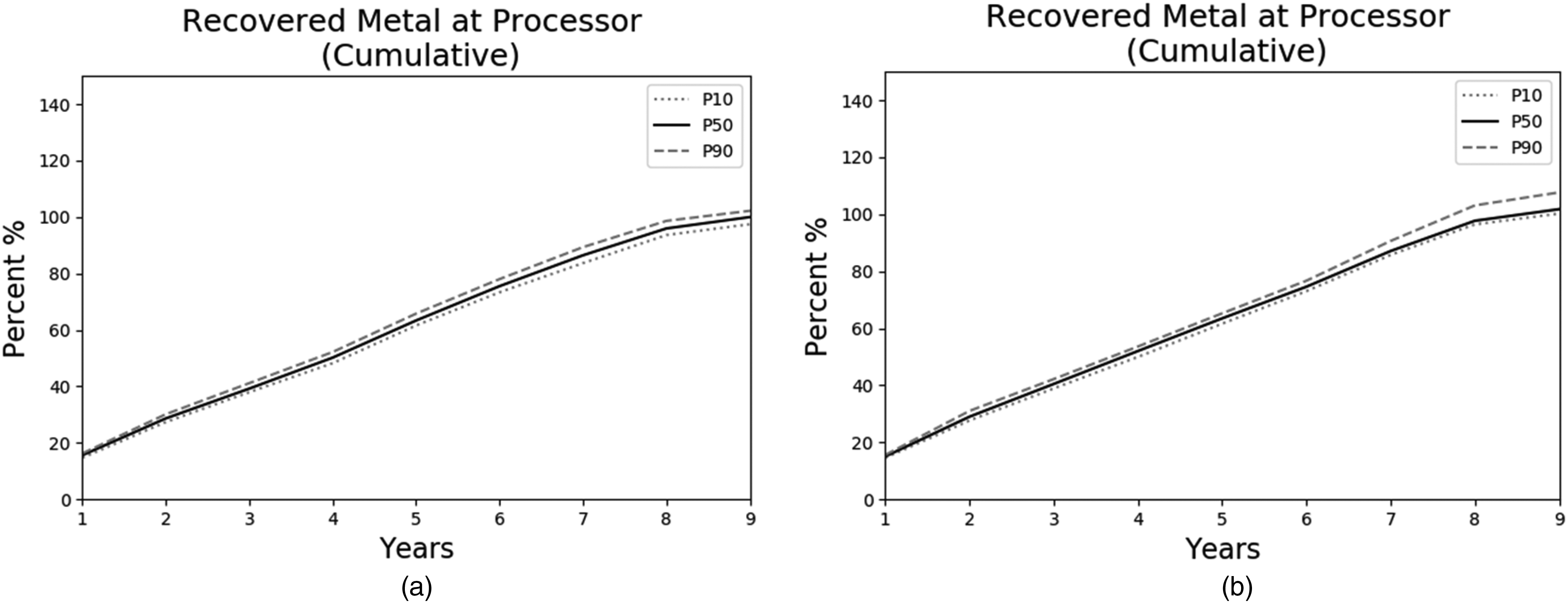
Scaled recovered metal forecasts from schedules obtained from (a) wireframed and (b) simulated geological domains. Values scaled using year nine in (a).

Figure 23.

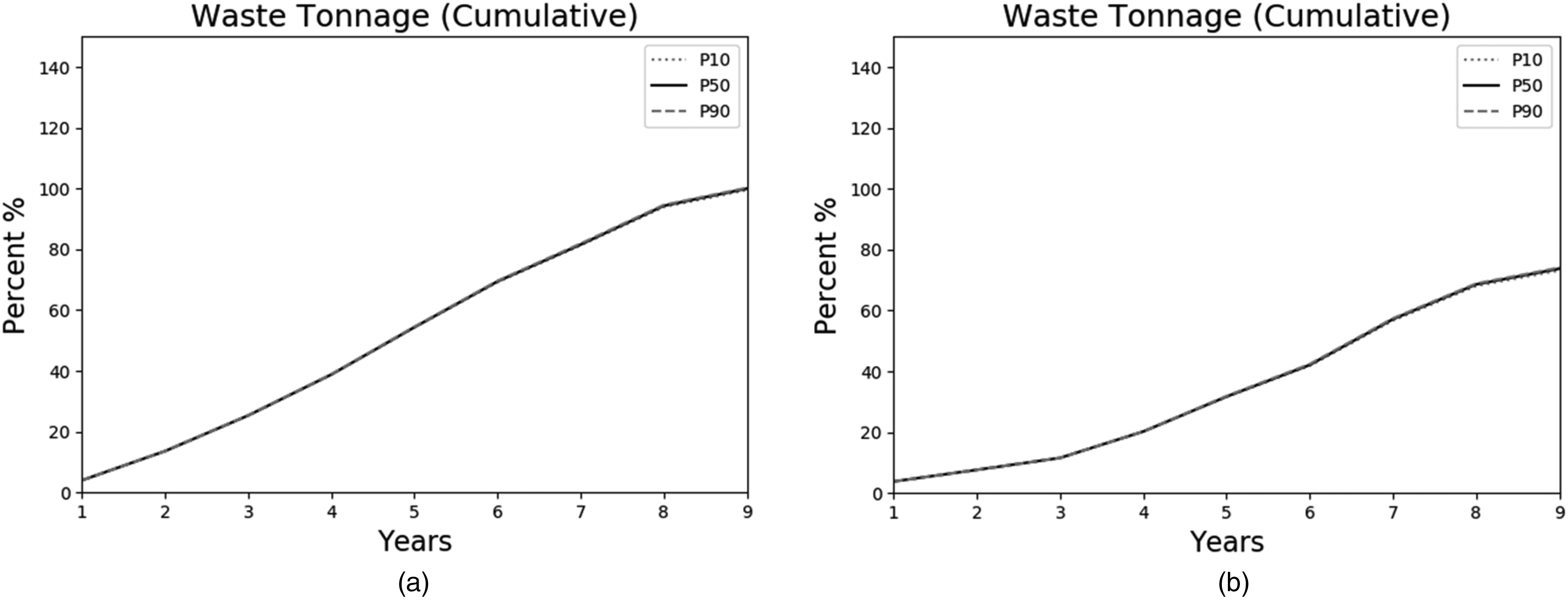
Scaled cumulative waste tonnage forecasts from schedules obtained from (a) wireframed and (b) simulated geological domains.

Figure 24.

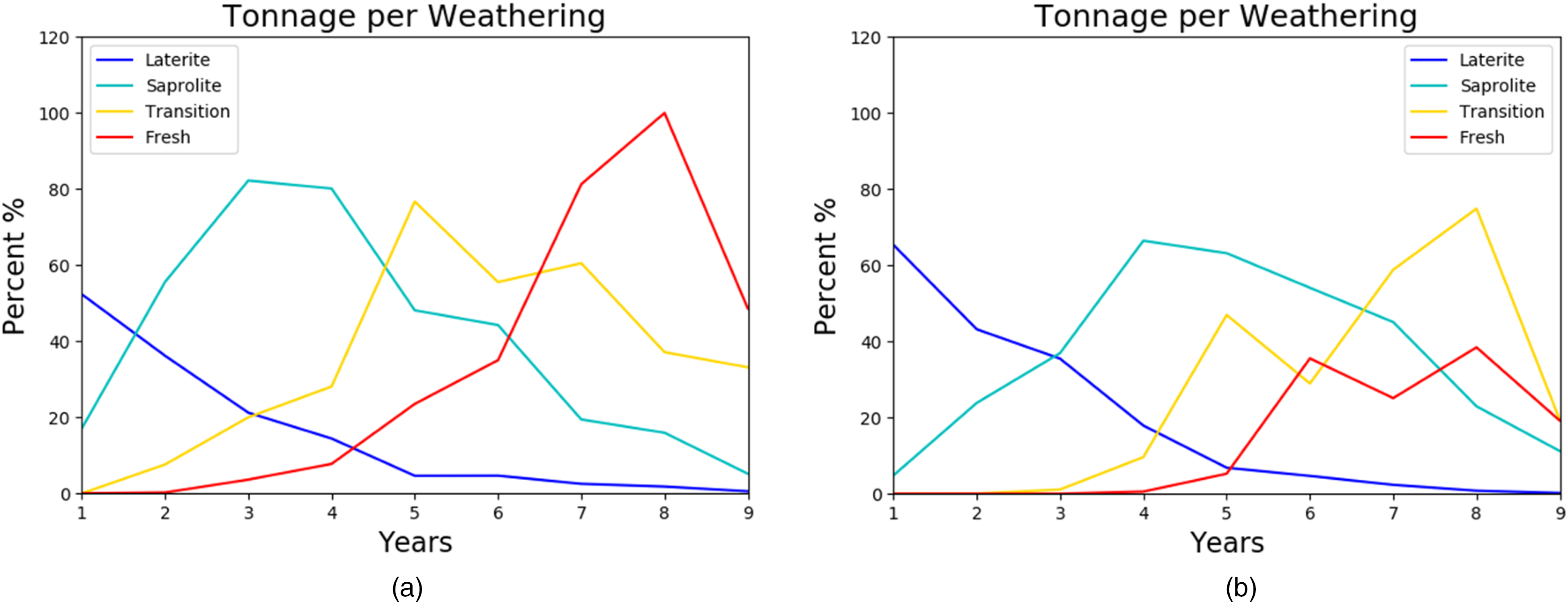
Scaled tonnage per weathering type from schedules obtained from (a) wireframed and (b) simulated geological domains.

Figure 25.

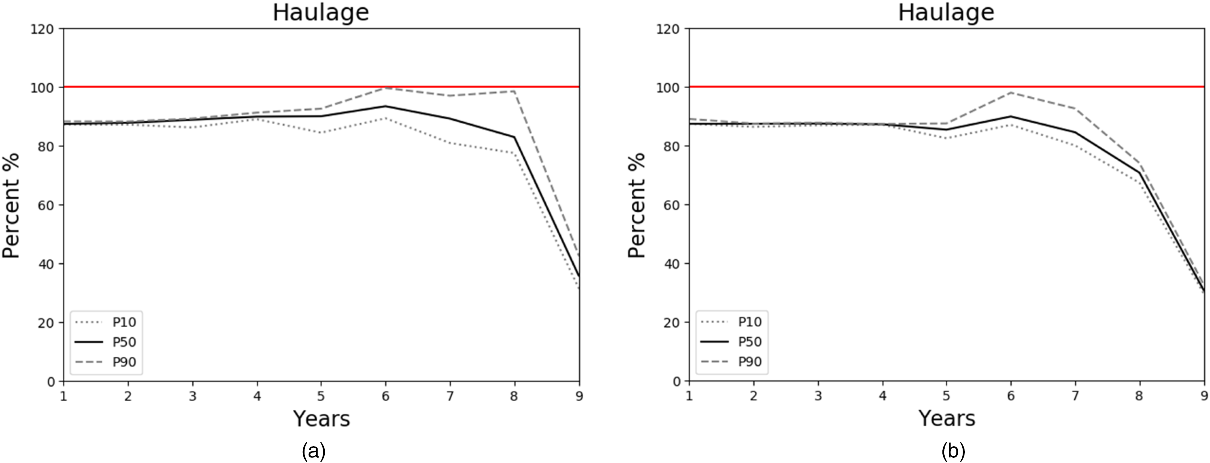
Scaled haulaged tonnes forecasts from schedules obtained from (a) wireframed and (b) simulated geological domains. Red lines indicate capacity constraint.

Figure 26.

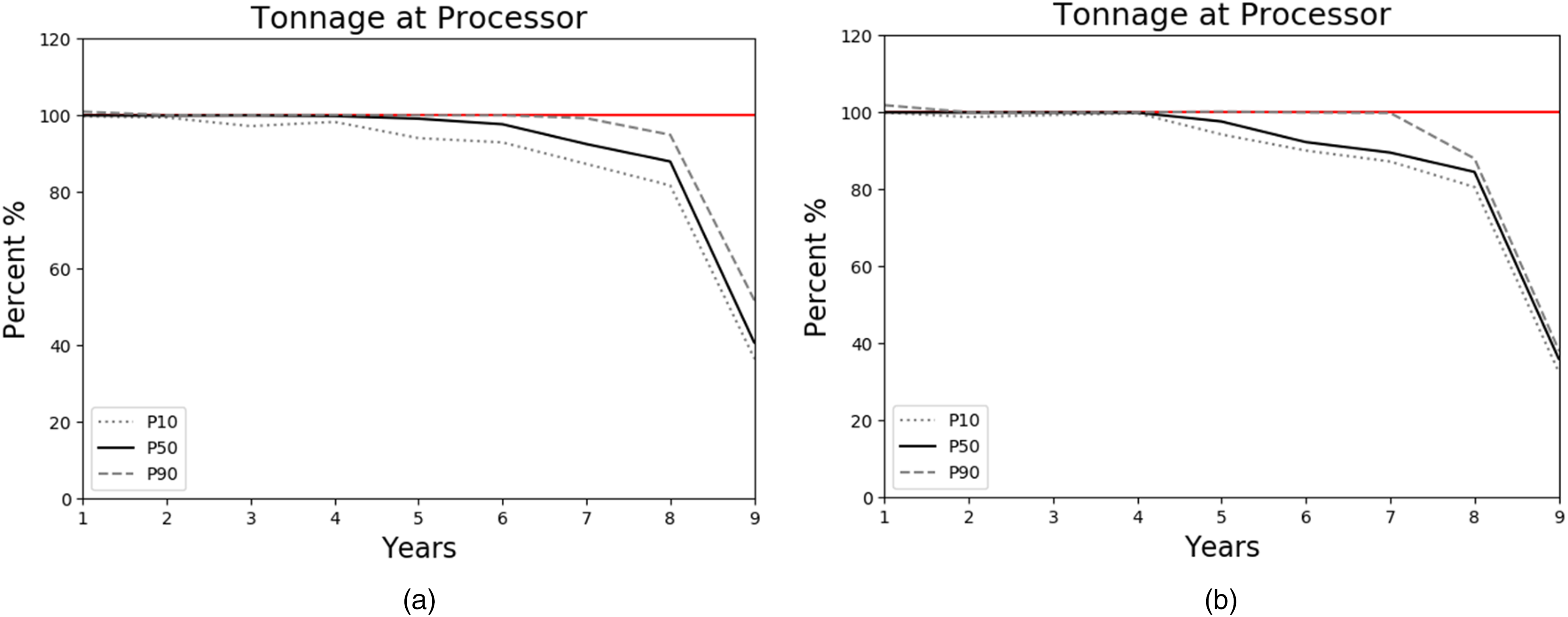
Scaled tonnes forecasts at processor from schedules obtained from (a) wireframed and (b) simulated geological domains. Red lines indicate capacity constraint.

Figure 27.

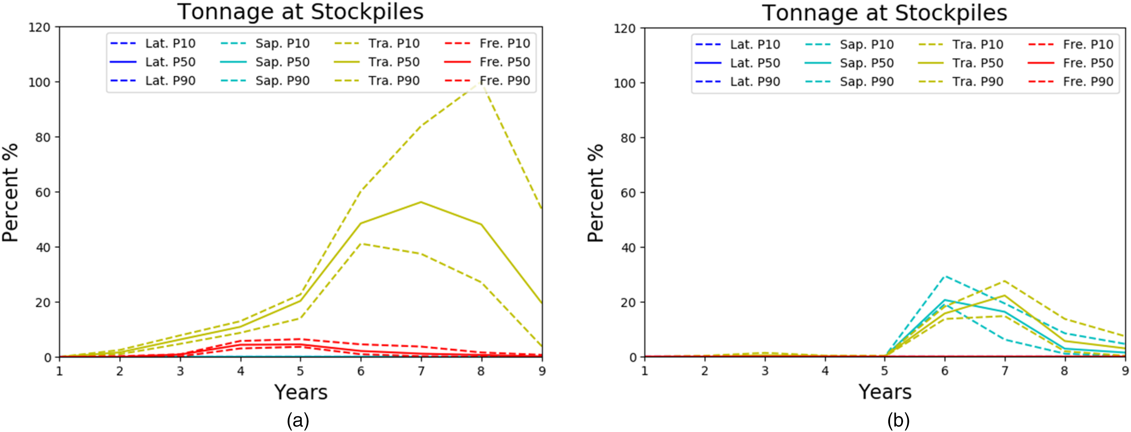
Scaled tonnes forecasts at stockpiles from schedules obtained from (a) wireframed and (b) simulated geological domains.

The forecasts for net present value (NPV) shown in Figure 21 present two noticeable differences. First, the widening of the risk profiles in Figure 21(b) for the schedule obtained based on simulated geological domains set. This widening corresponds to a 40% increase for year 9 (period of maximum NPV and mining stops), with respect to the NPV expected based on the wireframes. This result is expected, given that the additional source of geological uncertainty is accounted for, and it translates into more financial uncertainty with respect to the single wireframe-based schedule.

The second difference corresponds to a higher NPV reached by the schedule based on simulated geological domains. In this case, the increase corresponds to 20% with respect to the schedule based on wireframed domains. This effect is attributed to the ability of the optimisation process to capitalise over a representation of geological uncertainty and variability given by a set of realisations of geological domains and related boundaries, where simulated scenarios of geological domains replace the common single smooth wireframe representation of lithologies. To understand better this increase in value, more production forecasts are shown in Figures 22–27.

For the metal recovered at the processor shown in Figure 22, the two schedules present similar metal production at the mill. The only noticeable difference is, again, the widening in the risk profiles for the schedule based on simulated geological domains. As there are no major differences in cumulative metal production for the LOM, this is not the major cause for the difference in NPV noted between schedules. The difference is found in the waste tonnage handled by each schedule, shown in Figure 23. The schedule based on wireframed geological domains handles 25% more waste than the one based on simulated geological domains for the LOM. This difference is again attributed to the different spatial distributions of ore given by the simulation of lithologies, and to the simultaneous optimisation of cut-off grades given by the optimisation framework.

Another source for the difference in the expected NPV is attributed to the quantity of material types mined and the associated cost. Drilling and blasting costs for Fresh rock is five times higher than those for Laterite. As shown in Figure 24, the quantity extracted of Fresh in the schedule based on wireframed geological domains is higher than simulated ones, rendering a higher cost and respective reduction in NPV. The higher removal of Fresh rock also indicates that the schedule based on wireframed geological domains extracts more material at deeper levels, which can also be seen in Figure 20.

Regarding capacity constraints, Figures 25 and 26 show that both haulage and processing capacities are honoured. These figures also show the effect of the geological risk discounting, which allows for the management of risk by deferring it to later periods. This risk management is noticed by wider risk profiles in years 6, 7 and 8 than in the first four. The difference between the quantities shown in hauled and processed material is given by the material stockpiled, shown in Figure 27. Stockpiled material is also different for each schedule. The schedule based on wireframed geological domains stockpiles more quantity and more expensive material than the schedule based on simulated geological domains, helping to explain the difference in NPV forecasts.

Conclusions

The effects of the simulation of geological domains through the simultaneous stochastic optimisation of a gold mining complex were assessed and discussed. The optimisation method managed the geological uncertainty by maximising the NPV and minimising the risk of not meeting production targets and constraints, while capitalising in the synergies of the mine complex, for two sets of simulations: the first one based on a single wireframe, while the second based on simulations of geological domains.

The second set used 15 categorical scenarios of geological domains which were obtained through the high-order simulation method (HOSIM), without the use of a training image (TI). First- and second-order statistics of the fifteen realisations were validated by comparing them with corresponding data statistics. Similar validation was done for third- and fourth-order. The reproduction of statistics’ main patterns resulted as expected, given that HOSIM is a data-driven simulation method, rather than other TI-driven methods.

Validation of statistics (histograms and variograms) was also done for the simulation of gold grades within each mineralised geological domain. Grade simulations were obtained for wireframed and simulated geological domains.

The two sets of simulations were used as inputs to the simultaneous stochastic optimisation framework to obtain two schedules, respectively. The results observed by comparing both stochastic mine plans were: (a) different extraction sequences with consequently different ultimate pit limits, (b) 20% increase in expected NPV and 40% widening increase in the risk profiles when using the fully simulated geological set, (c) no major changes in metal recovered and (d) less handling of waste, with respective less cost, for the fully simulated geological set. These results stress the importance of accounting uncertainty and variability of geological domains in obtaining optimised mine plans.

The practical implications of these results start with the difference of extraction sequence and ultimate-pit limits, which are highly related to different mine designs and civil constructions such as ramps and the waste dump layouts. For the technical and financial forecasts, the widening of risk profiles is considered as a positive aspect because it implies a better accounting of geological uncertainty than only grade's uncertainty. The increase in 20% of expected NPV is considerable as for a gold project of this magnitude this percentage translates in the order of hundreds of millions of USD. Noticeable, this change in expected value does not come from more metal recovered, but for less waste handled, which also translates into volume reductions for the waste dump design and reduced environmental footprint.

For future work, for geological modelling, grades could also be simulated by HOSIM, as this method is known to represent better spatial connectivity of high grades. For mine-planning, multiple mineral deposits of the gold mining complex could be considered to fully capture the synergies of the mining complex, rendering an even higher economical value for the mining company. Considerations of gold price uncertainty could also be provided as it has increased substantially in the last years.

This manuscript has been derived from the work presented in Morales (2021).

Footnotes

Acknowledgments

Special thanks to Raphael Dutaut, Nathaniel Chouinard and Stephen Eddy from IAMGOLD for data and insights provided.

Data Availability Statement

The data is not publicly available due to confidentiality agreements.

Declaration of Conflicting Interests

The authors declared no potential conflicts of interest with respect to the research, authorship, and/or publication of this article.

Funding

The authors disclosed receipt of the following financial support for the research, authorship, and/or publication of this article: This research was supported by the National Science and Engineering Research Council of Canada (NSERC) CRD Grant CRDPJ 500414-16, NSERC Discovery Grant 239019 and the COSMO mining industry consortium (AngloGold Ashanti, Anglo American, BHP, De Beers, IAMGOLD, Kinross, Newmont Mining and Vale).

References

Albor

Dimitrakopoulos

(2009) Stochastic mine design optimisation based on simulated annealing: Pit limits, production schedules, multiple orebody scenarios and sensitivity analysis. Transactions of the Institutions of Mining and Metallurgy, Section A: Mining Technology 118(2): 79–90.

Armstrong

Galli

Beucher

, et al. (2011) Plurigaussian Simulations in Geosciences. 2nd ed. Berlin: Springer Verlag.

Barbaro

Ramani

(1986) Generalized multiperiod MIP model for production scheduling and processing facilities selection and location. Transactions of the American Institute of Mining, Metallurgical, and Petroleum Engineers, Society 280: 107–114.

Birge

Louveaux

(2011) Introduction to Stochastic Programming. 2nd ed. New York: Springer.

Boland

Dumitrescu

Froyland

(2008) A multistage stochastic programming approach to open pit mine production scheduling with uncertain geology. Optimization Online: 1–33.

Boucher

Dimitrakopoulos

(2009) Block simulation of multiple correlated variables. Mathematical Geosciences 41(2): 215–237.

Caumon

Collon-Drouaillet

Le Carlier De Veslud

, et al. (2009) Surface-based 3D modeling of geological structures. Mathematical Geosciences 41(8): 927–945.

Del Castillo

Dimitrakopoulos

(2019) Dynamically optimizing the strategic plan of mining complexes under supply uncertainty. Resources Policy 60(C): 83–93.

Dimitrakopoulos

(2011) Stochastic optimization for strategic mine planning: a decade of developments. Journal of Mining Science 47(2): 138–150.

10.

Dimitrakopoulos

Farrelly

Godoy

(2002) Moving forward from traditional optimization: Grade uncertainty and risk effects in open-pit design. Institution of Mining and Metallurgy. Transactions. Section A: Mining Technology 111: 82–88.

11.

Dimitrakopoulos

Lamghari

(2022) Simultaneous stochastic optimization of mining complexes - mineral value chains: An overview of concepts, examples and comparisons. International Journal of Mining, Reclamation and Environment 36(6): 443–460.

12.

Dimitrakopoulos

Luo

(2004) Generalized sequential Gaussian simulation on group size v and screen-effect approximations for large field simulations. Mathematical Geology 36(5): 567–591.

13.

Dimitrakopoulos

Mustapha

Gloaguen

(2010) High-order statistics of spatial random fields: Exploring spatial cumulants for modeling complex non-Gaussian and non-linear phenomena. Mathematical Geosciences 42(1): 65–99.

14.

Dimitrakopoulos

Ramazan

(2008) Stochastic integer programming for optimising long term production schedules of open pit mines: Methods, application and value of stochastic solutions. Transactions of the Institutions of Mining and Metallurgy, Section A: Mining Technology 117(4): 155–160.

15.

Dowd

(1994) Risk assessment in reserve estimation and open-pit planning. Transactions of the Institution of Mining and Metallurgy, Section A: Minerals Industry 103: A148–A154.

16.

Dowd

(1997) Risk in minerals projects: analysis, perception and management. Transactions of the Institution of Mining and Metallurgy, Section A: Minerals Industry 106: A9–A18.

17.

Farmer

Dimitrakopoulos

(2018) Schedule-based pushback design within the stochastic optimisation framework. International Journal of Mining, Reclamation and Environment 32(5): 327–340.

18.

Goodfellow

Dimitrakopoulos

(2016) Global optimization of open pit mining complexes with uncertainty. Applied Soft Computing Journal 40: 292–304.

19.

Goodfellow

Dimitrakopoulos

(2017) Simultaneous stochastic optimization of mining complexes and mineral value chains. Mathematical Geosciences 49(3): 341–360.

20.

Goovaerts

(1997) Geostatistics for Natural Resources Evaluation. New York: Oxford University Press.

21.

Guardiano

Srivastava

(1993) Multivariate geostatistics: beyond bivariate moments. In: Soares

(ed.) Geostatistics Troia ‘92, vol. 5. Dordrecht: Kluwer Academic Publishers, 133–144.

22.

Hoerger

Bachmann

Criss

, et al. (1999a) Long term mine and process scheduling at Newmont’s Nevada operations. 28th APCOM Symposium, 739–748.

23.

Hoerger

Seymour

Hoffman

(1999b) Mine planning at Newmont’s Nevada operations. Mining Engineering 51(10): 26–30.

24.

Irakarama

Laurent

Renaudeau

, et al. (2020) Finite difference implicit modeling of geological structures. Mathematical Geosciences 53: 785–808.

25.

Jewbali

Perry

Allen

, et al. (2018) Applicability of categorical simulation methods for assessment of mine plan risk. In: Dimitrakopoulos

(ed.) Advances in Applied Strategic Mine Planning. Cham: Springer, 513–536.

26.

Journel

(1983) Nonparametric estimation of spatial distributions. Mathematical Geology 15(3): 445–468.

27.

Journel

(1994) Modeling uncertainty: Some conceptual thoughts. In: Dimitrakopoulos

(ed.) Geostatistics for the Next Century. Dordrecht: Springer, 30–43.

28.

Journel

Alabert

(1989) Non-Gaussian data expansion in the Earth Sciences. Terra Nova 1(2): 123–134.

29.

Lamghari

Dimitrakopoulos

(2020) Hyper-heuristic approaches for strategic mine planning under uncertainty. Computers and Operations Research 115: 1–18.

30.

Lamghari

Dimitrakopoulos

Ferland

(2014) A variable neighbourhood descent algorithm for the open-pit mine production scheduling problem with metal uncertainty. Journal of the Operational Research Society 65(9): 1305–1314.

31.

Levinson

Dimitrakopoulos

(2020) Simultaneous stochastic optimisation of an open-pit gold mining complex with waste management. International Journal of Mining, Reclamation and Environment 34(6): 415–429.

32.

Mai

Topal

Erten

, et al. (2019) A new risk-based optimisation method for the iron ore production scheduling using stochastic integer programming. Resources Policy 62(June 2017): 571–579.

33.

Mariethoz

Caers

(2015) Multiple-point Geostatistics: Stochastic Modeling with Training Images. John Wiley & Sons.

34.

Mariethoz

Renard

Straubhaar

(2010) The direct sampling method to perform multiple-point geostatistical simulations. Water Resources Research 46(11): 1–14.

35.

Matheron

Beucher

de Fouquet

, et al. (1987) Conditional simulation of the geometry of fluvio-deltaic reservoir. In: 62nd Annual Technical Conference and Exhibition of the Society of Petroleum Engineers, pp.591–599. Dallas: Society of Petroleum Engineers.

36.

Minniakhmetov

Dimitrakopoulos

(2022) High-order data-driven spatial simulation of categorical variables. Mathematical Geosciences 54(1): 23–45.

37.

Montiel

Dimitrakopoulos

(2013) Stochastic mine production scheduling with multiple processes: Application at Escondida Norte, Chile. Journal of Mining Science 49(4): 583–597.

38.

Montiel

Dimitrakopoulos

(2015) Optimizing mining complexes with multiple processing and transportation alternatives: An uncertainty-based approach. European Journal of Operational Research 247(1): 166–178.

39.

Montiel

Dimitrakopoulos

(2017) A heuristic approach for the stochastic optimization of mine production schedules. Journal of Heuristics 23(5): 397–415.

40.

Montiel

Dimitrakopoulos

(2018) Simultaneous stochastic optimization of production scheduling at Twin Creeks Mining Complex, Nevada. Mining Engineering 70(12): 48–56.

41.

Montiel

Dimitrakopoulos

Kawahata

(2016) Globally optimising open-pit and underground mining operations under geological uncertainty. Transactions of the Institutions of Mining and Metallurgy, Section A: Mining Technology 125(1): 2–14.

42.

Morales

(2021) High-order Simulation of Geological Domains of a Gold Deposit and its Effects on the Simultaneous Stochastic Optimization of a Mining Complex. Montreal: McGill University.

43.

Mustapha

Dimitrakopoulos

(2011) HOSIM: A high-order stochastic simulation algorithm for generating three-dimensional complex geological patterns. Computers and Geosciences 37(9): 1242–1253.

44.

Newman

(2006) A survey of the marching cubes algorithm. Computers and Graphics (Pergamon) 30(5): 854–879.

45.

Payeur

Dutaut

Doucette

, et al. (2018) Technical Report On The Rosebel Gold Mine, Suriname, NI 43-101.

46.

Pimentel

Mateus

Almeida

(2010) Mathematical models for optimizing the global mining supply chain. In: Barin

(ed.) Intelligent Systems in Operations: Methods, Models and Applications in the Supply Chain. Hershey: IGI Global, 133–163.

47.

Ramazan

Dimitrakopoulos

(2007) Stochastic optimisation of long-term production scheduling for open pit mines with a new integer programming formulation. In: Dimitrakopoulos

(ed.) Orebody Modelling and Strategic Mine Planning. Uncertainty and Risk Management Models, vol. 14. Cham: Springer, 385–391.

48.

Ramazan

Dimitrakopoulos

(2013) Production scheduling with uncertain supply: A new solution to the open pit mining problem. Optimization and Engineering 14(2): 361–380.

49.

Ravenscroft

(1992) Risk analysis for mine scheduling by conditional simulation. International Journal of Rock Mechanics and Mining Sciences & Geomechanics Abstracts 101: A104–A108.

50.

Remy

Boucher

(2009) Applied Geostatistics with SGeMS: A User’s Guide. Cambridge: Cambridge University Press.

51.

Strebelle

(2002) Conditional simulation of complex geological structures using multiple-point statistics. Mathematical Geology 34(1): 1–21.

52.

Vallée

(2000) Mineral resource + engineering, economic and legal feasibility = ore reserve. CIM Bulletin 93(1038): 53–61.

53.

Whittle

(2007) Global asset optimisation. In: Dimitrakopoulos

(ed.) Orebody Modelling and Strategic Mine Planning: Uncertainty and Risk Management Models. Carlton: AusIMM, Spectrum Series 14, pp.331–336.

54.

Whittle

(2014) Not for the faint-hearted. In: Dimitrakopoulos

(ed.) Orebody Modelling and Strategic Mine Planning Symposium. Perth: The Australian Institute of Mining and Metallurgy, 3–5.

55.

Whittle

(2018) The global optimiser works-What next? In: Dimitrakopoulos

(ed.) Advances in Applied Strategic Mine Planning. Cham: Springer, 31–37.

56.

Zhang

Switzer

Journel

(2006) Filter-based classification of training image patterns for spatial simulation. Mathematical Geology 38(1): 63–80.

57.

Zuckerberg

Stone

Pasyar

, et al. (2007) Joint ore extraction and in-pit dumping optimisation. In: Dimitrakopoulos

(ed.) Orebody Modelling and Strategic Mine Planning. Uncertainty and Risk Management Models. 2nd ed., Vol. 14. Carlton: AusIMM, 137–140.

High-order simulation of geological domains and effects on stochastic long-term planning of mining complexes

Abstract

Keywords

Introduction

Methods

High-order simulation of geological domains

DBSIM of grades

Simultaneous stochastic optimisation of mining complexes

Application: Case study at the Saramacca gold deposit

Stochastic simulation of the Saramacca gold deposit

Simultaneous stochastic optimisation of the mining complex

Conclusions

Footnotes

Acknowledgments

Data Availability Statement

Declaration of Conflicting Interests

Funding

References