Evaluating Cognitive Models With Permutation Testing: A Case Study of Prototype and Exemplar Categorization

Abstract

Computational cognitive models offer powerful means for testing competing theoretical frameworks. A central challenge is determining which model best explains observed data, balancing goodness of fit with parsimony. Several fruitful approaches to model comparison have been used in the areas of cognitive and mathematical psychology, but the most popular in practice remain Akaike information criterion (AIC) and Bayesian information criterion (BIC), which penalize model complexity as measured by the number of free parameters. Here, we revisit these conventional approaches to model selection on a sample case of the prototype and exemplar models of categorization. We highlight the limitations of parameter count-based complexity measures, showing that they may fail to capture a model’s true flexibility. We then introduce a Monte Carlo permutation-testing approach as an alternative that has a rich tradition in many areas but whose use for model selection is still trailing that of AIC/BIC. We demonstrate that permutation testing offers at least three advantages: more robust comparison of models with chance, more robust comparison between models with equal or differing numbers of parameters, and quantification of uncertainty in model selection. After demonstrating how permutation testing offers a more nuanced and principled framework for evaluating cognitive models, we conclude with practical considerations for implementing permutation-based model selection in cognitive-modeling research.

Mathematically formalized cognitive models provide fundamental insight into the psychological processes underlying cognition and behavior (Farrell & Lewandowsky, 2018; Lee & Wagenmakers, 2013). They can be used to predict behavior, test competing theoretical assumptions, or bridge empirical observations with theoretical frameworks (Lewandowsky & Oberauer, 2018; Pitt et al., 2002). Ideally, cognitive models account for psychological processes in terms of a parsimonious set of parameters that can be interpreted as cognitively meaningful constructs (Schurr et al., 2024). Thus, cognitive models aimed at understanding human cognition have remained steadily popular ever since the publication of the first Handbook of Mathematical Psychology (Estes, 1964).

When considering two or more competing models of behavior, what is the best way to select among them? Optimization techniques, available in most software packages, can easily provide a goodness-of-fit metric, such as likelihood or mean squared error, for any model. However, what goodness-of-fit value is “good” when considering a single model? And how does one use model-fit values for comparison between models with an equal or different number of parameters?

Simple to compute and widely accepted, traditional model-selection criteria—especially Akaike information criterion (AIC; Akaike, 1974) and Bayesian information criterion (BIC; Vrieze, 2012)—address the balance of model fit with model complexity by penalizing models for each of their free parameters. Although many other approaches have been proposed (J. I. Myung & Pitt, 2004; Pitt & Myung, 2002), AIC and BIC remain the most commonly reported in cognitive-science publications over the past decade. A brief search with the term “computational modeling” in two example journals, Cognition and Journal of Experimental Psychology: Learning, Memory, and Cognition, reveals that in research in which model comparison was performed, 47% and 50% of articles in each journal, respectively, relied on AIC or BIC. When considering only studies predicting categorical rather than continuous response (the domain of application for AIC/BIC), we found that the percentage increases to 65% to 66% in each journal, respectively. However, equating model complexity with the number of free parameters is necessarily oversimplified (e.g., Hastie et al., 2009; Pitt & Myung, 2002; Villarreal et al., 2023). The implicit assumption that each parameter contributes equally and independently to model flexibility is often violated in cognitive models in which parameters may be constrained, hierarchically structured, and/or functionally redundant (Farrell & Lewandowsky, 2010; I. J. Myung, 2000). Thus, two models with the same number of parameters may differ in flexibility, whereas models with more parameters may in practice be more constrained.

In this tutorial-style article, we provide an introduction to an alternative approach: permutation testing. Permutation testing is a nonparametric method for hypothesis testing that is light on assumptions, flexible, intuitive, and widely accepted (Berry et al., 2011; Good, 2000; Pesarin & Salmaso, 2010). It has been used extensively to establish statistical significance in many domains that deal with complex, interdependent data (neural-population coding, Koren et al., 2020; Mendoza-Halliday & Martinez-Trujillo, 2017; Michaels & Scherberger, 2018; functional-MRI activation or connectivity, Eklund et al., 2011; Nichols & Holmes, 2002; Suckling & Bullmore, 2004; Suckling et al., 2006; electroencephalogram decoding, Hubbard et al., 2019; Li et al., 2022; Meyer et al., 2021). However, it has been underused for model selection. Here, we start by reviewing the traditional approaches to model fitting and model selection, AIC and BIC, on a sample case of the prototype and exemplar models of categorization. Readers well versed in prototype and exemplar models and/or traditional model fitting can choose to skim some of these background sections, but our goal was to provide enough context for both experienced and novice modelers. We then illustrate several weaknesses of traditional approaches to penalizing extra parameters, demonstrating that the amount of flexibility each additional parameter brings may not be well captured by the fixed penalization. We demonstrate how computationally intensive methods, such as permutation testing, may provide a more robust way to approach model selection. We demonstrate advantages of permutation testing for comparison of a single model with chance and its advantages for comparison of two models of interest. We describe how permutation testing helps with quantification of uncertainty in model selection. We then discuss several practical aspects of model selection in the area of categorization and cognitive modeling more broadly. We conclude by pointing interested readers to other resources and approaches to model selection. Although running thousands of simulations for each participant and each model would not have been realistic a few decades ago—leading to the adoption of computationally light heuristics—such simulations can nowadays be easily carried out on personal computers while providing a more robust means for evaluating model fits.

Prototype and Exemplar Models

Mathematical modeling has played a crucial role in understanding how humans learn concepts and organize their experiences into categories (for an overview, see Pothos & Wills, 2011). By simulating and predicting behavior, such models offer insights into the cognitive processes and representations that underlie categorization. Two foundational models in this domain are the exemplar and prototype models. The exemplar model postulates that individuals store detailed memories of specific category instances and make generalization decisions by comparing new stimuli with these stored exemplars (Curtis & Jamieson, 2019; Nosofsky, 1986, 1987; Zaki et al., 2003). In contrast, the prototype model suggests that people abstract a central tendency—a prototype—from multiple experiences and use this summary representation to guide categorization (Posner & Keele, 1968). Although many sophisticated categorization models have been proposed (Ashby et al., 1998; Kurtz, 2007; Love et al., 2004; Nosofsky et al., 1994; Tenenbaum & Griffiths, 2001), here, we use prototype and exemplar models as two competing accounts of how people represent concepts because they provide a convenient means for illustrating mathematical model fitting and comparing traditional and permutation-testing approaches with model selection. We focus on fitting models to trial-by-trial responses from individual participants rather than to aggregated data because aggregation can obscure individual differences and distort the underlying cognitive representations (Ashby et al., 1994). However, we conclude with a brief discussion of how the same permutation-testing approach can be applied when fitting continuous data, such as group averages.

The exemplar model originated from Medin and Schaffer’s (1978) context model. The context model stated that the psychological similarity between two stimuli is context dependent. For example, a mug and a bottle may be judged as highly similar in a context that emphasizes function but highly dissimilar in a context that emphasizes structure. Nosofsky (1986) introduced a generalized version (generalized-context model) that captures context dependency with selective attention weights that can systematically modify the shape of psychological space in which stimuli, or exemplars, are embedded. Effectively, psychological space is stretched along attended dimensions and shrunk along less attended or ignored dimensions. Attended dimensions are typically those learned to be category relevant, and ignored dimensions are those that are category irrelevant, but other goals or prior biases also play a role in how attention is directed to stimulus features. The exemplar model predicts category judgments by mapping a novel stimulus into psychological space and computing its similarity to each stored exemplar within the relevant categories. These similarities are summed within each category and compared to determine the most likely classification.

The prototype model makes many of the same assumptions as the exemplar model (Wattenmaker et al., 1986). However, categories are assumed to be represented by their prototypes, or summary representations of the exemplars that have been encountered (Posner & Keele, 1968). Prototypes are usually operationalized as the mean or mode of feature frequencies. To make categorization decisions, similarity is computed between a novel stimulus and each category’s prototype. Because a prototype is essentially the mean or mode of its exemplars, novel stimuli are often similarly related to both prototype and exemplar representations, leading to correlated model predictions (Mack et al., 2013). However, from the full pattern of responses, it is usually possible to determine which model provides a better account of behavior.

Calculating perceived similarity from physical and psychological distance between stimuli

Mathematical formalization of these models relies on characterizing the feature space of the stimuli, which allows one to quantify the physical distance between stimuli and its inverse, physical similarity. This is often achieved by constructing artificial stimuli with known dimensions. Especially popular are stimuli with binary-dimension features (Bowman & Zeithamova, 2018), which we also use here, although the similarity metrics have known adaptations for continuous-dimension stimuli (Kalish & Kruschke, 2000). In general, the physical distance between two stimuli (x, y) can be computed as

$$distance(x,y)={\left[\sum {\left|x-y\right|}^r\right]}^{\frac{1}{r}},$$

(1)

where x is a vector representing feature values of stimulus x, y is a vector representing feature values of stimulus y, and r is the distance metric. The distance metric is typically set to r = 1 for separable dimension stimuli, such as those with binary features, representing city-block distance. The sum is then simply the sum of differences (or lack thereof) across all stimulus dimensions. For example, imagine that stimuli have three binary features: size (large or small), color (black or white), and shape (triangle or circle). The distance (difference) between two stimuli can range from zero to three features. For example, large black triangle differs by one feature from small black triangle and by three features from small white circle. In general, the more features two stimuli have in common, the more similar they will be to each other and the smaller the distance between them. Formally, the large black triangle can be represented as a vector with values [0 0 0], the small white circle can be represented as a vector with values [1 1 1], and all other stimuli can be represented as a vector consisting of zeros or ones representing one or the other value on each dimension.

The distance metric can also be set to r = 2 for continuous, especially integral-dimension, stimuli, representing Euclidian distance. For example, imagine that stimuli are lines varying along two continuous value dimensions: length and orientation. A line with tilt of 50° and length 20 mm can be represented as a vector (50, 20), and a line with a tilt of 80° and length 60 mm can be represented as a vector (80, 60). Their Euclidean distance in vector space would be calculated as the square root of their squared differences on each dimension (30°, 40 mm), or $\sqrt{{\left(50-80\right)}^2+{\left(20-60\right)}^2}=50$ .

Although these formulas for physical distance provide a good illustration of the logic of the calculation, they do not account for the perceived, or psychological, distance without some adjustments. First, as demonstrated in the context model and others, it may be that not all stimulus dimensions are equally salient or equally attended by a subject. Moreover, 1 unit of change along one dimension may not be equivalent to 1 unit of change in another dimension, as would likely be the case for degrees of orientation and millimeters of length. Second, to estimate perceived similarity from distance, the models take into account research in psychophysics and especially the work of Shepard (1958, 1987) that showed that perceived similarity decays exponentially as a function of distance. Attention weights to each feature and the rate of decay of perceived similarity as a function of distance are not just features of the stimuli themselves but also a function of the observer and context, and they are thus not known a priori. However, they can be estimated from the responses of individual subjects.

Mathematical equations formalizing the prototype and exemplar models account for differential attention and the exponential decay of perceived similarity, and in their basic versions, prototype and exemplar models differ only in their assumption of how categories are represented. Prototype models assume that category structures are represented by their prototypes, and thus, they compute the similarity of each test stimulus to each category’s prototype. Perceptual similarity is modeled as an exponential decay function of physical similarity while taking into account differences in attention to specific features. Formally, the similarity $S$ of a test stimulus $x$ to Category A is

$$S_A(x)=\exp \left[-c{(\Sigma (w{\left|x-prot{o}_A\right|}^r))}^{\frac{1}{r}}\right],$$

(2)

where proto_A is a vector characterizing the prototype of Category A, $c$ is a sensitivity parameter that determines the rate of decay (estimated from the data), $r$ is the distance metric, and $w$ is a vector of attention weights with length equal to the number of stimulus features (estimated from the data and constrained to sum to 1).

Exemplar models assume that categories are represented by their exemplars, or individual instances observed during the training phase. These models calculate similarity between each stimulus and a category by computing the summed similarity of the stimulus and all the training stimuli from the given category (Nosofsky, 1986, 1987):

$$S_A(x)=\underset{y\in A}{\Sigma }\exp \left[-c{(\Sigma (w{\left|x-y\right|}^r))}^{\frac{1}{r}}\right].$$

(3)

Here, y represents a training stimulus from Category A, and all other parameters are the same as in the prototype model. Because there are typically several (potentially many) training stimuli in each category (as opposed to a single category prototype), similarity is computed to each of these training stimuli and summed across all of them.

Predicting the probability of each response

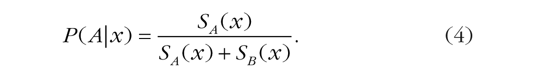
To transform these measures of psychological similarity to probabilities of each response, we use a commonly employed Luce choice rule (Luce, 1963) that estimates the probability of each response by dividing the similarity to the given category by summed similarity to all relevant categories. In the case of two categories, the probability of responding “A” on a given trial would be computed as the similarity to Category A divided by the sum of similarity to Category A and Category B:

$$P(A|x)=\frac{S_A(x)}{S_A(x)+S_B(x)}.$$

(4)

We discuss an alternative version of the exemplar model with a more complex version of the choice rule toward the end of the article. However, we start with the basic version as a convenient means to illustrate model fitting and model selection using traditional and permutation-testing approaches.

Model Fitting Using Maximum Likelihood Method

Once a model is specified mathematically, the typical next step is to estimate which values for the model’s parameters best reproduce the observed sequence of responses from a given subject (“best fit” approach). The most common metric for models that generate probability estimates is the maximum likelihood. To estimate the likelihood of a single response for a given model and a given set of parameters, we calculate the probability of the response that a subject actually selected on that trial. For example, assume that a model’s estimated probability of choosing “A” is 75% on the first trial and the probability of choosing “B” is the remaining 25%. If the subject chose “A” on the first trial, the likelihood of the subject’s response “A” is .75. If the subject chose “B,” the likelihood of the subject’s response is .25. Conceptually,

$$\begin{array}{c}P(actualresponse)=P(A|x)ifparticipantrespondedA\hfill \\ P(actualresponse)=P(B|x)ifparticipantrespondedB.\hfill \end{array}$$

(5)

Because each experiment typically involves many trials, the goal is not to predict just one decision but the whole sequence of a subject’s responses. For example, if the subject responded “A-B-B-A” across Trials 1 through 4, what would be a set of parameters generating predictions most closely matching all these responses?

Mathematically, the total likelihood of a given sequence of responses is equal to the product of likelihoods across all trials. For example, if the likelihood of a given subject’s response is 0.5 on Trial 1, 0.2 on Trial 2, 0.7 on Trial 3, and 0.6 on Trial 4, the likelihood of the given sequence of four responses is 0.5 × 0.2 × 0.7 × 0.6 = 0.042. Of course, to be able to compute the likelihood of each response, one needs to know the value of all parameters. In typical scenarios, the values of the parameters are not known a priori, so one has to use minimization algorithms, built into the majority of statistical-analysis tools, to find the set of parameters that maximizes the total likelihood of the given sequence of responses.

In practice, for anything more than a handful of trials, using the raw total likelihood computed as a product of probabilities across trials is not feasible. Because probabilities are between zero and one, multiplying many of them together can result in extremely small numbers that cannot be accurately represented in a calculator or computer and result in numerical instability. Instead, raw likelihoods for each trial are log transformed and then summed together, which is numerically stable, convenient, and mathematically equivalent: The logarithm of a product of a vector of numbers is equal to the sum of logarithms of individual numbers, ln(a × b) = ln(a) + ln(b). Because the likelihood is always a number between 0 and 1 on each trial, the log likelihoods are negative. Therefore, maximizing the likelihood estimate corresponds to maximizing the sum of negative numbers, making the sum as close to zero as possible. For convenience, it is standard to take the negatives of log likelihoods so that the optimization goal is to minimize the sum of positive numbers instead (again, making the sum as close to zero as possible). Most analysis tools have functions designed to achieve just that—minimization functions that search through parameter space to find a set of parameter values that make some outcome value as small as possible.

The results of model fitting are twofold. First, model fitting generates estimates of the model’s parameters that provide the best fit to the data, and the parameter values themselves are potentially of interest because they are thought to reflect underlying psychological processes. Second, model fitting generates the overall fit value (e.g., the maximum likelihood, or more commonly, the negative-log-likelihood value) that can be used to evaluate the overall model’s performance and serve as a basis for comparison of fits of multiple models against each other.

Traditional Approaches to Model Selection

After researchers fit a model and obtain a fit value, how do they know if a model fits the data “well”? And when they have two or more competing models, how do they decide which model fits “better”? Relying on a model’s raw fit value is usually not sufficient. Typically, models with more parameters fit data better than models with fewer parameters, but it may be due to overfitting—fitting the noise instead of (or in addition to) the signal (Villarreal et al., 2023). For example, any set of observations can be fit perfectly with a model that has the same number of parameters as there are observations, but such a model has no explanatory or predictive value. Therefore, the resulting likelihood value must be evaluated in the context of the model’s complexity, which is traditionally achieved by including some form of penalization for the total number of free parameters (Akaike, 1974; Schwarz, 2007; Vrieze, 2012). Usually, simpler models with fewer parameters are preferred over complex ones with more parameters unless substantial improvement in fits justifies the use of more complex models.

The two most used goodness-of-fit metrics are AIC (Akaike, 1974) and BIC (Schwarz, 2007). Other easy-to-compute goodness-of-fit metrics have been proposed, such as consistent AIC (Bozdogan, 1987) and Hannan-Quinn criterion (Hannan & Quinn, 1979), but they share the same parameter-penalization principle as AIC and BIC and are less used in practice. We thus focus on AIC and BIC, which are to this day the most popular metrics balancing fit with complexity. Both AIC and BIC involve computing the best-fitting (minimal) negative log likelihood, –ln(L), followed by an explicit penalization for the number of free parameters, but they were developed with somewhat different goals (Burnham & Anderson, 2004; Cavanaugh & Neath, 2019; Neath & Cavanaugh, 2012). We first focus on AIC. Akaike (1974) considered that fitting a model too closely to the data at hand could reduce its ability to generalize to future data drawn from the same underlying distribution. The proposed penalty for complexity was derived based on how much model fit tends to improve with each additional free parameter, assuming large samples. Based on these considerations, AIC is calculated as $-2\ln \left(L\right)+2k$ , where $k$ is the number of parameters. Models with lower AIC are considered better fitting. Under an assumption of large samples, the AIC penalization has been shown to favor models that best predict new data (Akaike, 1974; see also Cavanaugh & Neath, 2019; Neath & Cavanaugh, 2012).

In comparisons of two models that have the same number of free parameters (i.e., the versions of the prototype model and the exemplar model described above), the penalizations are often equal and thus cancel each other out, meaning one can simply choose the model with smaller negative-log-likelihood values, reflecting higher overall likelihood of the data given the model. When two models vary in the number of free parameters, the more complex model (model with more parameters) cannot just fit better; it must outperform the simpler model by a fit difference proportionate to the difference in the number of free parameters. We illustrate how the penalization works in a case in which we want to compare a cognitive model with chance. Traditionally, to model random behavior, we first construct a null model, also called a “random model” or a “flat model.” Such a model can have zero free parameters and simply assume that the probability of responding “A” on a given trial is always 0.5 for two categories. In other words, the null model with zero parameters assumes that a subject chooses randomly on every trial with each of the two responses having equal probability and with no regard to what stimulus is presented for categorization. The misfit of the model is always 0.5 on every trial because the prediction is 0.5 and the actual response is 0 or 1. Alternatively, the null model can incorporate a single bias parameter, which is estimated as the proportion of trials that a subject selected one response option over the other. Thus, the null model assumes that on every trial, $P(A)$ in Equation 5 equals the known proportion of “A” responses and $P\left(B\right)=1-P(A)$ equals the known proportion of “B” responses. For example, if the subject tended to respond “A” on 80% of trials, the null model assumes that—irrespective of what stimulus is being categorized—the probability of responding A is 0.8 on every trial and that the probability of responding “B” is 0.2. The negative log likelihood of the subject’s series of responses is calculated based on that prediction.

The null model typically fits worse than a more complex model, resulting in lower likelihood and higher (worse) negative log likelihood. However, to balance fit with complexity, the AIC requires the cognitive model of interest (e.g., the prototype or exemplar model) to outperform the null model by a certain value. For example, many prior studies used four dimensional stimuli, so the number of free attentional weights for the prototype model would be three (the attention to the fourth dimension is dictated by the remaining three because they sum to 1). One additional free parameter would be sensitivity c, for a total of four free parameters. Thus, AIC for the prototype (or exemplar) model would be calculated as AIC = −2 × ln(L) + 2 × k = −2 × ln(L) + 8, and AIC for the null model with a single bias parameter would be calculated as AIC = −2 × ln(L) + 2 × k = −2 × ln(L) + 2. The much larger penalty for the prototype model (eight) compared with the null model (two) dictates by how much the prototype model has to outperform the simpler model. Otherwise, the simpler null model will be favored, and the prototype model will not be considered fitting better than chance.

Similar to AIC, BIC, also known as Schwarz information criterion, is derived from the negative log likelihood combined with penalization for free parameters. However, the goal of BIC is to determine which of competing models would be most likely to produce the data at hand (Schwarz, 2007). BIC is calculated as $-2\ln \left(L\right)+k\times ln(n)$ , where k is the number of free parameters and $n$ is the number of trials/samples. Schwarz (2007) demonstrated that under certain assumptions, this penalization provides an efficient means for selecting the true model among the candidate models. Otherwise, the model-selection procedure is similar to using AIC: Compute BIC for all candidate models, often including a null model. Then, select model with the lowest (best) BIC as the winner. Because the penalization for free parameters is not fixed at 2 × k but instead scales (logarithmically) with the number of trials, the BIC penalty is typically more severe than that of AIC, more strongly favoring simpler models over complex ones. As a downside, such penalization may be too strict. Especially if the true model is not among the candidate models, BIC may underfit, missing important structure in the data, and is not guaranteed to generalize well out of sample. Furthermore, some of the assumptions of BIC are unlikely met in cognitive research, including the assumptions of large (asymptotically infinite) samples, independent contributions from each parameter, or the true model being among the candidate models (I. J. Myung, 2000).

AIC/BIC are easy to compute, useful in many contexts, and backed by information-theoretic principles (Akaike, 1974; Burnham & Anderson, 2004; Vrieze, 2012). Nevertheless, parameter-count-based penalization used by both AIC and BIC is necessarily oversimplified (Grünwald & Roos, 2019; I. J. Myung et al., 2000). There are at least two important issues with the assumption that the complexity of a model is fully determined by the number of its freely estimated parameters (also see Pitt & Myung, 2002; Villarreal et al., 2023). First, it assumes that the functional forms of models are all equivalent, meaning all else equal, one model’s functional form is not inherently more flexible than another’s. In addition, it assumes that each additional parameter affords the same flexibility both within a model and between models, which may not be the case. Instead, to better understand the complexity of a model, one should consider the distribution of predictions that a model can make, including determining whether the model can predict the specific responses of a subject better than it can predict mere noise (also see Palminteri et al., 2017; Pitt & Myung, 2002). This is at the heart of an alternative approach to model selection using permutation testing. Before explaining permutation testing in more detail, we briefly introduce the data sets used as a running example throughout the article.

Data Sets Used for Running Examples

We have completed the same method-evaluation analyses in several data sets from our lab with more than 600 participants (e.g., Bowman & Zeithamova, 2018, 2020, 2023), leading to the same conclusions. To illustrate the principles and advantages of permutation testing in this article, we model two large-N data sets, reported in Bowman and Zeithamova (2023). The first experiment (N = 177) used eight-dimensional binary-value stimuli, and the second experiment (N = 276) used 10-dimensional binary-value stimuli (e.g., square or round body, head forward or up; Fig. 1). The category structure was generally prototype-based such that no feature was necessary or sufficient but rather, the overall number of category-consistent features determined category membership. Each experiment used multiple category structures varying in the number and typicality of training exemplars across participants, allowing us to compare model-fitting approaches across a wider range of parameters than if we relied on just one experiment.

Fig. 1.

Stimulus structure. Example stimuli used in the study by Bowman and Zeithamova (2023) that provided data reported here. Stimuli varied along eight and 10 binary features in Experiments 1 and 2, respectively. Prototypes for two categories differed on every dimension. Example stimuli between category prototypes have different numbers of features shared with their prototype, representing their varying physical similarity to the prototype.

All participants completed a category-learning phase in which they learned to categorize a set of training exemplars into one of two categories via corrective feedback. Participants then completed a recognition-memory test (not discussed further in the current article) and a no-feedback categorization test with old and new category exemplars. Prototype and exemplar models were fit to the categorization-test data. For both data sets, $r$ was fixed to 1, assuming a city-block distance metric. The number of stimulus features in Experiment 1 was eight, and in Experiment 2, it was 10. Thus, for both models, there are nine or 11 subject-specific parameters estimated from subjects’ pattern of responses: one sensitivity parameter c and eight or 10 attention weights w (one for each stimulus dimension). Consistent with standard modeling approaches, we assume that attention is a finite resource and that all stimulus features compete for a shared pool of attention, instantiated in both models as a constraint that the attention weights across all features sum to 1 (Minda & Smith, 2001). In this case, each attention weight can be interpreted as the percentage of one’s attention allocated to a given feature. As a result, estimating all but one attention weight determines the attention allocated to the final weight, and the number of attention-weight parameters considered free to vary will always be one fewer than the number of stimulus features. Thus, for traditional approaches to model selection, we assumed eight free parameters in Experiment 1 (one parameter c, seven attentional weights free to vary) and 10 free parameters in Experiment 2. Because the two experiments had a different number of test trials, the raw fit-value distributions will be distinct between experiments, although this distinction does not necessarily indicate better or worse fit to the different data sets in general.

The original data from Bowman and Zeithamova (2023), the stimuli, and the scripts for model fitting and permutation testing are all available at https://osf.io/5pdw3/files/osfstorage. The link also contains eight-dimensional stimuli from Experiment 1 recoded from 10-dimensional to a more intuitive eight-dimensional notation. To create eight-dimensional structure, the original 10-dimensional notation had two dimensions (leg width and foot shape) perfectly correlated and the color dimension fixed at gray (Fig. 1). Although MATLAB (The MathWorks, Natick, MA) was used to run all analyses in the current article, we additionally provide an R script that replicates the same analyses. Furthermore, we provide an R package designed specifically for categorization-related computational modeling, including functions for running prototype and exemplar models as discussed above (https://github.com/troyhouser/CatMod).

Permutation-Testing Approach to Model Selection

Permutation testing is a specific application of the Monte Carlo method, which is a broad class of computational algorithms that rely on repeated random sampling for estimating probabilities (Ernst, 2004; Good, 2000; Holt & Sullivan, 2023). For example, to estimate the probability of getting a tail when tossing a coin, one may toss a coin 10,000 times, count the total number of tails across all tosses, and use the relative frequency as an estimate of the probability of getting a tail. Perhaps one may get 5,017 tails and 4,983 heads across the 10,000 tosses for the estimated probability of a tail being 5,017 ÷ 10,000 = 0.5017, or 50.17%.

Of course, most would be happy to accept that the probability of a tail is half, or 50%, without requesting to see results of 10,000 tosses. However, other situations are much more difficult to decide a priori based solely on theoretical considerations. Thus, when analyzing data that are unsuitable for standard statistical tests because of complexity and lack of normality, various Monte Carlo–based approaches, such as permutation testing or bootstrapping, provide a robust means for evaluating statistical significance and estimating p values (Henderson, 2005; Ludbrook, 1994). Permutation testing is a robust nonparametric statistical method that involves repeatedly shuffling or permuting data labels, such as responses on each trial, to simulate the null hypothesis, or expected distribution of an outcome if there was no real signal in the data. Permutation testing has been the go-to method of evaluating significance with complex data and/or when parametric assumptions may not be met (Pesarin & Salmaso, 2010). The examples range from neuroimaging (Eklund et al., 2011; Nichols & Holmes, 2002; Suckling & Bullmore, 2004; Suckling et al., 2006) to machine-learning model validation (Diciccio et al., 2020; Ojala & Garriga, 2010) to biomedical research (Ludbrook & Dudley, 1998) to economics (Bugni et al., 2023). In the remainder of this section, we demonstrate how permutation testing can be used for evaluating model fits and show its advantage over traditional model-selection approaches. Similar to traditional approaches, permutation testing can be used to assess whether a cognitive model fits data better than chance and to compare two competing models with the same or different number of free parameters. We then describe how to use permutation testing for each of these model-evaluation tasks and illustrate with examples why permutation approach often yields a more robust result than traditional methods.

Comparison with chance

The first question one should ask when using a formal model is whether the model meaningfully accounts for a subject’s behavior. Is there any evidence that the subject engaged in the processes that the model assumes? Or do their responses appear more or less random? Although the comparison with chance is sometimes skipped when comparing two competing cognitive models is of interest, we advocate that a comparison with chance should be always included as the first step. For instance, it may be misleading to assign one or the other cognitive strategy to a subject who does not appear to use any strategy at all.

Using accuracy to determine whether a subject responded randomly is less straightforward than it may seem. First, one needs to decide what level of performance is “chance.” Sometimes, “above chance” is defined as more than 50% correct for two categories. Alternatively, we consider that even accuracies above 50% can be still obtained just by chance. A cutoff criterion in such cases would typically be based on a binomial distribution, which evaluates the probability of a given number of correct out of total responses given a probability of random success on each trial. For example, 60% categorization accuracy may or may not be considered above chance depending on the sample size: Six or more out of 10 correct is fairly likely to happen just by chance (about 38% probability) but 60+ out of 100 is fairly unlikely to happen just by chance (about 3% probability). However, with a smaller number of trials, such a criterion may be rather strict. Moreover, and perhaps most relevant for the current topic, a participant may be using a consistent strategy, but the strategy does not align with the experimenter-defined categories. In such a case, a model may describe participants’ behavior well even when their accuracy is at chance. Thus, when categorization strategies are of interest, researchers typically use model-comparison tools rather than accuracy to evaluate behavior against chance.

With traditional approaches, one typically evaluates cognitive models against chance by constructing a null model and then comparing the AIC/BIC value of the null model with the AIC/BIC value of the cognitive model(s) of interest. The null model simply becomes one of the models a researcher is comparing. The permutation-testing approach is a bit different. Rather than constructing the null model, one instead constructs a null distribution of model fits for each candidate model. This allows directly taking into account the given model of interest and the given subject’s pattern of responses. How well would this model fit if this subject was responding randomly to these stimuli? Is their actual model fit any better than what would be expected by chance?

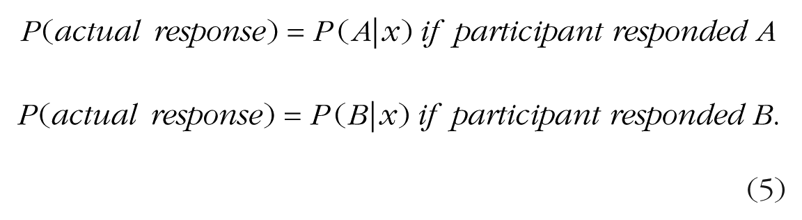
Permutation testing allows us to answer these questions by repeatedly simulating random responses and fitting the model into those random responses, recording the overall model fit for each simulation. With enough simulations, we construct the null distribution of model fits and can then directly compare this distribution with the observed model fit obtained from the subject’s real data. To obtain each random simulation for a given subject, our recommended approach is to keep the stimuli that the subject encountered and keep the subject’s actual responses but randomly shuffle the stimuli and the responses with respect to each other. A simple way to achieve it in a computer simulation is to randomly permute the responses that the subject gave while leaving the stimuli in order (Table 1). This produces a randomized data set in which there is no real relationship between the stimuli and the responses, so whatever fit value we obtain to this randomized data, it is obtained just by chance. Shuffling the stimuli with respect to responses would produce equivalent results because prototype and exemplar models are not influenced by the order of the stimulus-response pairs. Another option would be to generate a completely random sequence of responses, such as flipping a (virtual) coin on each trial and assigning “A” and “B” responses randomly based on heads or tails. However, shuffling the subjects’ actual responses has the advantage of maintaining any response bias the subject might have had while still randomizing the relationship between a stimulus and its response. This provides a better estimate of what “chance” is for a given subject because predicting responses for someone who tended to choose Category A on 80% of trials may be easier than predicting responses of someone who distributed responses more evenly.

Table 1.

Illustration of the Permutation Approach to Creating Each Simulation

Actual data		Example Simulation 1
Stimulus value	Subject response	Stimulus values	Permuted subject responses
1 1 1 0	A	1 1 1 0	A
0 1 0 0	B	0 1 0 0	A
0 0 0 1	B	0 0 0 1	B
0 1 1 1	A	0 1 1 1	A
0 0 0 0	B	0 0 0 0	A
1 0 0 0	A	1 0 0 0	B
1 1 0 1	A	1 1 0 1	B

Note: Example using stimuli that vary along four binary dimensions (four features, each with two possible values). Stimulus values are represented as vectors of ones and zeros, one value for each feature. To generate the subject-specific null distributions, we use the stimuli that the subject encountered and the subject’s actual responses but randomly shuffle the stimuli and the responses with respect to each other. This produces a randomized data set in which there is no real relationship between the stimuli and the responses but the type of stimuli encountered in an experiment and any potential response biases are maintained. By repeating the simulation many times, with a new randomized data set for each simulation, one can obtain a subject-specific null distribution of random model fits for each model.

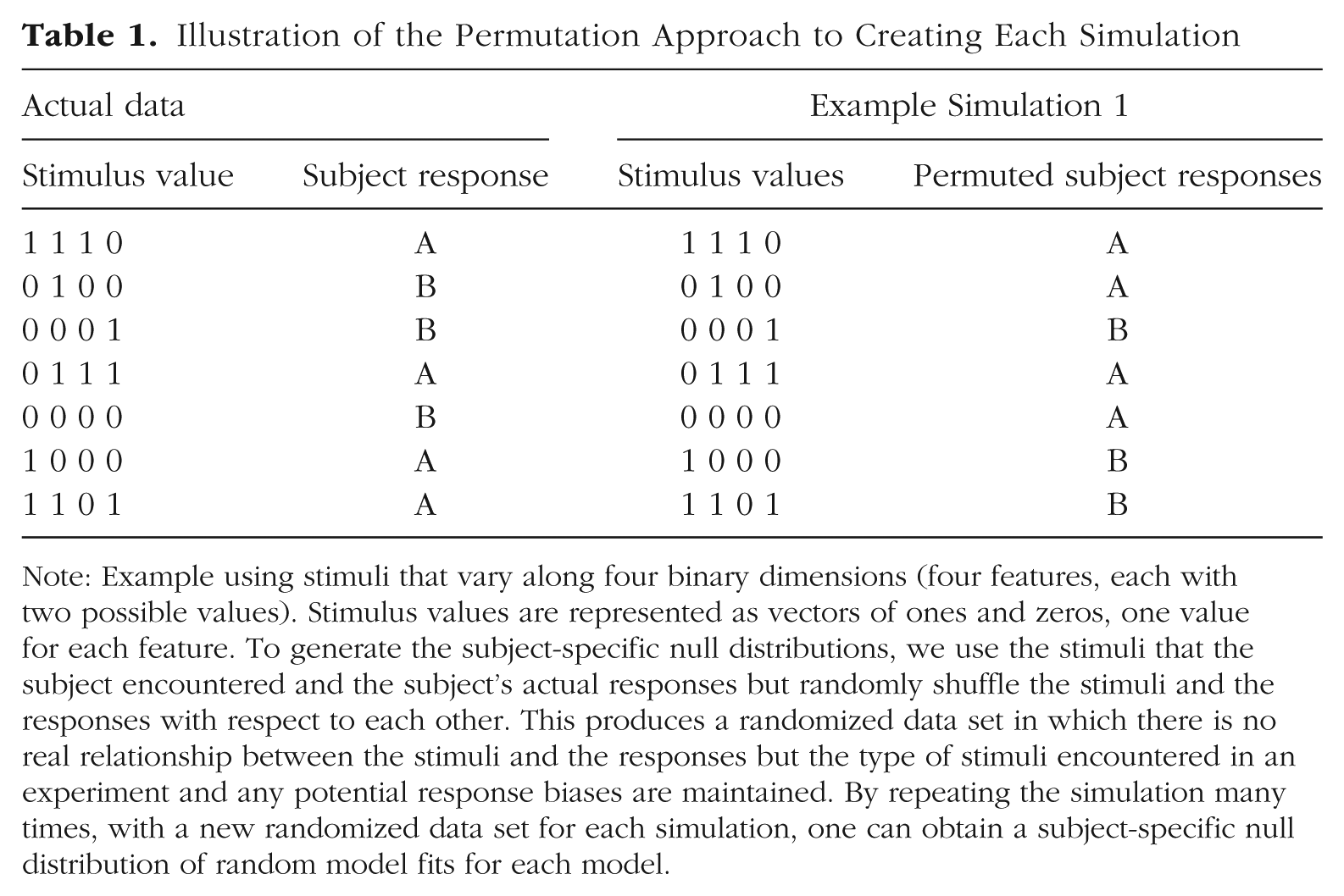
Once we complete a large number of simulations (we use 10,000 in this article but demonstrate that fewer may be sufficient), followed by model fitting into each simulated data set, we can generate the subject-specific null distribution of model fits. The null distribution provides information about the typical range of model-fit values that happen for that model just by chance, when the underlying data contain no real signal. Figure 2 shows such null distributions for the prototype and exemplar models for two example subjects from our prior study (Bowman & Zeithamova, 2023). The distributions, represented by the histograms, show the range of fit values we should expect just by chance, that is, if the subject was responding randomly rather than using any strategy.

Fig. 2.

Distributions of randomly simulated model fits. Example subject-specific null distributions of model fits for (left; red) exemplar model and (right; blue) prototype model for two example subjects, one in each row. To generate each subject’s null distributions, we randomly shuffle the order of their categorization responses with respect to the stimuli and then fit the prototype and exemplar models to this random data, storing the resulting fit values. This procedure is repeated 10,000 times for each subject to generate the subject’s null prototype and exemplar fit distributions. The null distributions, depicted by the red or blue histogram, show the range of fit values that would be expected just by chance, if there was no real relationship between the stimuli and responses. We then consider where the actual fit to the subject’s real data falls with respect to the null distribution. Here, the observed fit (fitting real subject’s data) is denoted by vertical dotted lines. Most commonly, the observed fit is considered better than chance if it appears in the corresponding null distribution with a frequency less than 5% (p < .05, one-tailed). Here, the subject depicted in the top row has both model fits well above chance (exemplar model: p < .001; prototype model: p < .001). In contrast, the actual fit value for the subject depicted in the bottom row does not appear reliably above chance because it occurs frequently just by chance (exemplar model: p = .274; prototype model: p = .162).

The dotted lines in Figure 2 represent the actual model fit for a given subject (lower = better). Comparing each subject’s observed prototype and exemplar model fits with their subject-specific prototype and exemplar null distributions allows us to determine whether one or both models fit the subject’s data better than chance. The relative frequency of model fits as good or better than the observed one estimates the likelihood that a given fit can be obtained just by chance. In other words, it represents the empirically derived p value of the model fit such that low p values indicate that the fit is statistically significantly above chance (i.e., unlikely to happen just by chance). Large p values indicate that the fit is not particularly good and can frequently be observed just by chance even if responses were completely random.

The top row of Figure 2 represents one subject who did not appear to respond randomly. The subject’s observed prototype model-fit value (negative log likelihood) was 10.05. None of the 10,000 simulations yielded a prototype fit as good or better than the actually observed one (lower value = better fit), meaning that such a good prototype model fit can be observed just by chance with p < .0001. Likewise, the exemplar model fit is also very unlikely to be this good just by chance (fit = 11.02, p < .0001). Thus, we would conclude that the models perform better than chance. To put it differently, assuming that the subject responded using one of those strategies accounts for the subject’s data far better than assuming the subject responded randomly.

In contrast, the bottom subject in Figure 2 had a prototype model fit of 39.71, with 1,620 of 10,000 random simulations yielding fits as good or better than the actually observed one (p = .162). Their exemplar model fit was also observed relatively frequently just by chance (fit = 40.00, p = .274). Thus, assuming that the subject followed a prototype or exemplar strategy does not seem to account for the subject’s data significantly better than assuming that the subject responded randomly.

The two subjects depicted in Figure 2 were selected to be clear-cut, and most subjects in our recent studies have been clear-cut as well. In general, whether the responses appear random is easier to distinguish when a larger number of responses are fit. It can be more difficult to confidently discern random responses from strategy-following responses when fitting only a few trials. Nevertheless, in every study, one has to choose a cutoff threshold for all the subjects as to what is considered above-chance model fit. In our prior work, we have typically used a threshold borrowed from null hypothesis testing and considered a model to fit data better than chance if it outperforms 95% of random simulations (p < .05, one-tailed, that the fit is this good just by chance). For example, a subject’s observed exemplar model fit would be considered better than chance if fewer than 5% of the random simulations (from the subject’s exemplar null distribution) produced fits that were as good or better as the observed data fit. The prototype model fit would be evaluated against the null distribution of prototype model fits. Subjects for whom neither model outperformed chance would be labeled as responding randomly (classified as “chance” or “neither [model]”). Nevertheless, it may be reasonable to use a different cutoff threshold, depending on the study goals.

Advantages of permutation approach for comparing with chance

The first advantage of permutation testing is that it can quantify the uncertainty of the comparison with chance in terms of probability. Although setting a threshold (e.g., p < .05) for comparison with chance when using the permutation approach is inevitably arbitrary, researchers can use it to their advantage and adjust the threshold based on the question of interest. For instance, we may use a more stringent threshold when the goal would be to select only the subjects fit by the model very well or a more lenient threshold when the goal is to screen out only a minimum number of subjects whose data appear most obviously random. Importantly, we argue that AIC/BIC also sets a threshold, determined by the penalization of extra free parameters, but without a way to quantify the uncertainly associated with that threshold.

Second, permutation testing accounts for the actual model flexibility in a more precise manner than that achieved by counting free parameters. This is an important point for both the comparison with chance and comparison between models. AIC and BIC both penalize for the number of free parameters in the models, using a fixed penalty for each free parameter (AIC) or a fixed penalty for each parameter whose value is proportionate to the number of trials (BIC). This requires making an assumption about how much flexibility (fit improvement) each extra parameter contributes just by chance. However, as we illustrate, such assumptions do not always match reality. It is not the case that each added parameter provides the same additional flexibility. Nor is it the case that two models with equal number of parameters are equally flexible. And finally, in the case of some models, it is not even clear how many free parameters there really are. For example, if there are constraints on any model parameters (e.g., attention weights constrained between 0 and 1 and summing to 1 in the prototype and exemplar models), the number of effective free parameters will be smaller than the nominal number of parameters. Thus, although the free-parameter penalization in AIC and BIC metrics is well validated and has been shown to provide sensible outcomes, we argue that it can be too lenient or too severe in many cases.

Importantly, comparing with chance using permutation testing requires a model to outperform itself when fit into randomized data, bypassing all of these challenges. Does the model do a better job accounting for a real person’s data than random junk data? If a model is excessively flexible, able to account for any pattern of data, then it will be just as successful fitting junk (randomized) data as fitting real data. If constraints or other model features make it less flexible than what the nominal number of parameters would suggest, this will also be true for that same model fit to random data. Although the number of trials fit and the number of free parameters will always affect the fit value in potentially complex ways, these are always equated when fitting the actual versus simulated data with the exact same model. Thus, one does not have to make a priori assumptions about the exact cost one should associate with free parameters within the realm of other constraints. Instead, the Monte Carlo simulations provide a much better estimate of the “ground truth” of model flexibility than any theoretical assumption.

We first illustrate the problem with counting free parameters and expand on it with actual data in the next paragraph. First, consider that prototype and exemplar models both estimate an attentional weight for each stimulus dimension. This may not be a problem for stimuli with three or four dimensions because the free-parameter penalty will be relatively small, but several studies have used stimuli with a higher number of dimensions to create a larger number of unique stimuli. For example, in our prior work (Bowman et al., 2020, 2022; Bowman & Zeithamova, 2018, 2020, 2023), we used stimuli with eight or 10 dimensions. AIC and BIC both penalize for the number of free parameters in the models. Because one attention parameter is estimated for each stimulus feature, this penalty can be quite severe for high dimensional stimuli, such as the eight- and 10-dimensional stimuli used in those studies. As we illustrate below, these metrics then label a large proportion of subjects as responding randomly, including some subjects whose categorization accuracy appeared to be above chance.

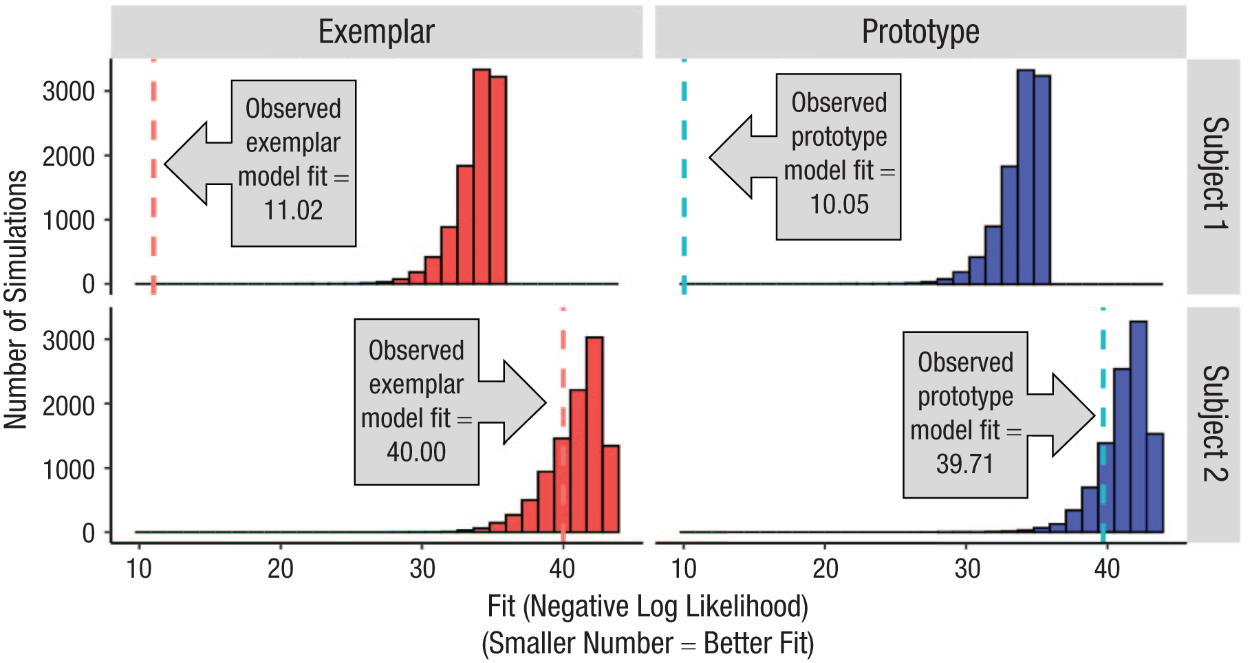
In Experiment 1 in Bowman and Zeithamova (2023), we used eight dimensional stimuli. Because the attentional weights always sum to 1, one can safely consider only seven free parameters representing the attentional weights because the last attentional weight is fully dictated by the first seven. There are further constraints on the weights, such as that they are bound between 0 and 1, making it unlikely that seven is the right number of truly free parameters. However, there is no clear way to adjust the number of free parameters to account for such a constraint. Thus, we end up with a severe penalty for eight “free” parameters for the prototype and exemplar models (7 attentional weights + 1 c parameter) in comparison with the null (random) model that contains only a single parameter P (probability of responding “A”). Once penalized for the many free parameters using AIC or BIC metric, many subjects’ fits would not be considered above chance because AIC/BIC fit values were better (lower) for the random model than the prototype and exemplar models. For example, one subject from Experiment 1 categorized stimuli with 68% accuracy, which is reliably above chance (50%, binomial test p = .017), yet this subject would be classified as “chance” had we not used permutation testing. The subject’s AIC values were 47.72 for the random model, 50.33 for the exemplar model, and 49.32 for the prototype model, leaving the random model as the winner. The BIC values were even more extreme in favor of the random model. However, once we construct the empirical null distribution of the model fits expected if the subject were responding randomly, we see that the subject’s fit value is rather unlikely to happen by chance (Fig. 3). The raw exemplar-model fit value (negative log likelihood) was 17.17. A fit value this good or better appeared in only 12 out of 10,000 simulations, translating to a probability p = .0012 that a fit as good or better can arise just by chance. The prototype-model null distribution had even fewer simulated fits (seven out of 10,000) as good or better than the empirically observed prototype fit (prototype fit = 16.66, p = .0007). Thus, both accuracy and permutation testing suggest that this subject was not responding randomly.

Fig. 3.

Illustration of AIC/BIC over penalization. Example subject whose responses are best fit by the random model when AIC or BIC is used for model selection but who was unlikely to be responding randomly once we consider what random fit looks like using a Monte Carlo approach. (a) Distribution of simulated exemplar model fits. (b) Distribution of simulated prototype model fits. Vertical dashed lines are empirically observed model fits.

The illustrative subject was not a single exception. Using AIC and BIC for model selection (prototype, exemplar, random) would lead to a larger portion of subjects being best fit by the random model than when we use the permutation approach. For example, in Experiment 1, the permutation approach identified 28 out of 176 subjects as responding randomly, but AIC labeled 45 subjects as responding randomly, and BIC labeled 69 subjects as responding randomly. In Experiment 2, permutation approach identified 73 out of 276 subjects as responding randomly, but AIC labeled 97 as responding randomly, and BIC labeled 134 subjects as responding randomly. With one exception (one out of N = 452 across both studies), every subject who was labeled as responding randomly per the permutation approach was also best fit by the null model when using AIC/BIC model comparison. However, some subjects who were labeled as “chance” by AIC/BIC were assigned a strategy when using the permutation test for model selection (their model fits were considered above chance). When looking at the performance of these subjects in terms of accuracy, we find it is unlikely they were responding randomly. In Experiment 1, the average categorization accuracy of subjects labeled random by AIC and BIC but not permutation testing was 60% and 65%, respectively. In Experiment 2, the average categorization accuracy of subjects labeled random by AIC and BIC but not permutation testing was 59% and 65%, respectively. It is unlikely to achieve these scores if these subjects were choosing randomly (choice of two categories, chance = 50%).

These results suggest that the traditional metrics can be overly conservative in distinguishing prototype and exemplar models from the random model, especially for models with higher number of free parameters or models that include parameter constraints. Importantly, permutation testing gives the most accurate estimate of the “ground truth” of what a distribution of chance fits looks like irrespective of how many parameters there are in the model, working just as well with few or many parameters. Although AIC or BIC metrics can serve as useful, computationally fast heuristics in many cases, permutation testing will provide a more precise answer in many real-world applications.

Comparison between two cognitive models: Is zero really the point of no difference?

In addition to allowing one to better differentiate strategic responses from chance, the permutation approach allows one to make a more informed decision between two models (e.g., the prototype and the exemplar models) when comparing them directly. The AIC/BIC metrics consider only the number of parameters when determining whether one model outperforms the other and not necessarily the degree of flexibility those parameters provide. As we demonstrate, two models with the same number of parameters are not necessarily equally flexible, and one may be more likely to fit better even when fitting random data. Furthermore, model-fit differences differ in magnitude, making it difficult to decide whether small differences are meaningful.

First, we probe the assumption of the AIC/BIC approach to model selection that focuses on the number of free parameters. For any two models that have the same number of parameters, the penalization for free parameters cancels out, and one can simply compare raw model fits –ln(L) between the two models to determine the winner. To apply this notion to the prototype and exemplar models, consider the following: If the prototype model’s fit (negative log likelihood) is better (lower) than the exemplar model’s fit, then the prototype model wins. If the exemplar model’s fit is better (lower) than the prototype model’s fit, then the exemplar model wins. The two models would be considered to fit equally well if they have the same fit value, or a difference in fit value of zero.

We examine this assumption that the cutoff point of deciding in favor of one or the other model should be zero difference between the two model fits, which implicitly assumes that the functional forms of both models are equally flexible. To do so, we again consider how well the individual models can fit just by chance and how the two model fits can differ from each other just by chance. Figure 4 shows the key null distributions that we consider during model selection for a representative subject. Figure 4a shows the null distributions of exemplar model fits, Figure 4b shows the null distribution of prototype model fits from a representative subject, with information added about the subject’s central tendency statistics. From these distributions, we may already suspect that despite equal number of parameters, the two models are not necessarily equally flexible. The average fit to randomized data was 24.00 for the exemplar model and 24.86 for the prototype model. The median fit to randomized data was 24.34 for the exemplar model and 25.22 for the prototype model. Thus, even when fitting random data with no real signal, the exemplar model tends to be more successful in accounting for the pure noise and “fit better” on average.

Fig. 4.

Systematic fit differences occurring just by chance. Top figures are null distributions of model fits (model fits to shuffled subject responses). (a) Exemplar (red) model fits. (b) Prototype (blue) model fits. (c) Null distribution of raw model-fit differences (exemplar model fits minus prototype model fits). Vertical dotted lines denote the average (or median in the bottom figure) fit of the null distribution, and solid vertical lines denote the empirically observed fits. All data are from a single representative subject.

This can be even better illustrated when we consider a new null distribution: the null distribution of model-fit differences (Fig. 4c). Each data point on this distribution is the signed difference between exemplar model fit and the prototype model fit to the same randomized data (exemplar – prototype), as obtained during one of the 10,000 simulations we ran for that subject. Negative numbers represent better exemplar model fit (exemplar model having lower fit error), and positive numbers represent better prototype model fit (prototype model having lower fit error). As we show in the distribution, some randomly simulated data end up better fit by the prototype model, and some end up better fit by the exemplar model. The distribution is centered close to zero but not exactly zero despite the 10,000 data points it is based on. In fact, as is visualized in Figure 4c, there is a relatively substantial amount of negative skew in this distribution. For this subject, both the mean and median of the null distribution of model-fit differences was negative (−0.86 and −0.50, respectively). These numbers may seem small, but they are reliable: The mean fit difference was −0.83 versus −0.88 for the first 5,000 versus second 5,000 simulations, respectively; the median difference was −0.47 versus −0.53 for the first versus second 5,000 simulations, respectively. If we were to assign a strategy to each simulated data set, we would find that only 3,095 of the 10,000 raw fit differences (31%) favor the prototype model and that 6,380 (64%) favor the exemplar model. The remaining 5% of simulations resulted in equal prototype and exemplar fit (with equality evaluated to five decimal points). Thus, the exemplar model was twice as likely to outperform the prototype model when fit into random-noise data despite the fact both models have an equal number of parameters.

The above consideration is at the heart of permutation-testing approach to model selection. Instead of just looking at the model-fit differences, one can consider how likely the model-fit differences are to arise by chance alone. The simplest option of how to decide in favor of one model over the other would be to compare the observed model-fit difference (exemplar – prototype) with the mean or median of the null distribution of model-fit differences as a more valid cutoff point compared with using zero. For example, we could consider −0.50 or −0.83 as better cutoff points for model selection than 0. In general, if we observe a model-fit difference that falls in the center of the null distribution of model-fit differences, such a difference is likely to arise by chance, and it may not be appropriate to classify the subject as using the exemplar or the prototype strategy. We may decide that the model fits are too similar to call a winner and instead conclude that both models fit the given subject about equally well. In contrast, if we see a difference that is more extreme than most of the difference scores that appear by chance, we may feel confident that one model indeed outperformed the other (see also Cox, 1962). Importantly, we should consider the actual null distribution rather than assuming that it must be centered at zero.

For the subject depicted in Figure 4, the observed model difference (exemplar – prototype) is +0.63, indicating that the prototype model fit better. Although we would likely consider this subject a prototypist with or without seeing the subject’s null distribution of model-fit differences, considering the full null distribution of model-fit differences allows us to make an even better informed decision of which differences to consider meaningful or large enough to warrant confident classification. Here, the fit difference of +0.63 in favor of the prototype model appears by chance in only 13% of simulations. Thus, we may be relatively confident in the subject’s strategy classification. In contrast, had we observed a model-fit difference of −0.63, seemingly in favor of the exemplar model, we should not be confident in classifying the subject as an exemplarist. Considering the subject’s null distribution, we would see that nearly half (47%) of the random simulations show equal or larger fit differences in favor of the exemplar model just by chance. Thus, such a value would likely not be enough evidence for confident classification.

Importantly, just like with the raw model fits, the range of model-fit differences that we expect to observe just by chance will vary based on the specific stimuli the subject encountered, the number of trials the subject responded to, the number of trials the subject missed (if any), and the subject’s response bias. When we construct subject-specific null distributions of model-fit differences for all the subjects from a given study, we can see that the subject-specific null distributions may not all be biased the same way. Figure 5 illustrates the distributions of the central tendencies (mean and median) of model-fit differences that we observed in Bowman and Zeithamova (2023) across hundreds of subjects. Values away from the zero difference illustrate the bias of one model fitting better than the other just by chance. As shown in Figure 5, midpoints of the null distributions were close to zero for many subjects, but there were also many subjects whose null distributions were decidedly not centered at zero. As the negative skew indicates, when random simulations favored one model more over the other on average, it was always the exemplar model in our data set. The estimates of the midpoints of the subject-specific null distributions were highly reliable within subjects: Reliability ranged between 0.974 and 0.999 for medians and means across the two experiments, computed as a correlation between midpoints estimated from the first 5,000 simulations and second 5,000 simulations. Thus, the center of the null distribution being offset from zero was not driven just by random noise. Rather, it demonstrates inherent differences in the flexibility of the two models.

Fig. 5.

Distribution of model biases across all subjects. (Left) Mean and (right) median simulated model-fit differences across all subjects from (top) Experiment 1 and (bottom) Experiment 2. Fit differences are exemplar model fit minus prototype model fit. Because smaller value means better fit, the negative values for many subjects indicate that the exemplar model tended to fit random data better than the prototype model in those subjects.

Across all subjects in our experiments (Fig. 5), we observed a bias for the exemplar model to fit the randomized responses better than the prototype model (Experiment 1, exemplar advantage: Mdn = −0.07, M = −0.20; one-sample t test comparing mean with 0 (no bias): t[175] = −10.694, p < .001; Experiment 2, exemplar advantage: Mdn = −0.02, M = −0.23; one-sample t test comparing mean with 0, t[275] = −15.577, p < .001). That is, even when no real relationship existed between the stimuli and the responses in the simulated random data, the exemplar model systematically fit better than the prototype model for many subjects. Thus, two models with the same number of parameters may not be equally flexible because one can fit even pure noise better than the other model.

Clearly, assuming that the null difference in model fits is zero for models with equal number of parameters is not warranted. Importantly, we also observed variability in the magnitude and direction of the fit bias across subjects and conditions, suggesting there is no one-size-fits-all solution to accounting for the potential differences in model flexibility. The variability of bias across participants was driven by differences between category structures and test stimuli they encountered and thus may be difficult to predict from one study to the next. Instead, considering the subject-specific null distribution of model-fit differences provides a way to evaluate such a bias, incorporating any effects of category structure, number of trials, response biases, and so on in a data-driven manner. Importantly, the same procedure using null distributions of model-fit differences can be used when models differ in their number of parameters, bypassing the challenge of a priori deciding how much each parameter should be penalized.

Realistically accounting for extra free parameters: the case of gamma

The traditional approach to model comparison assumes that a model’s flexibility is determined by the number of free parameters, with explicit penalization for extra free parameters required for models that differ in the number of free parameters. So far, we have illustrated two challenges to this approach. First, the penalization may be too strict when there are many parameters, parameter constraints, and/or interdependencies, as illustrated by the challenge of comparing the prototype and exemplar models with chance. Second, two models that have an equal number of parameters may not be equally flexible in practice, with a bias for one model to fit any pattern of data better than the other model—even when the data are pure noise. In this section, we illustrate another example of when fixed penalization of extra free parameters may lead to undesirable outcomes. Specifically, we discuss a case in which a theoretically motivated addition of a free parameter to one model may lead to overall worse performance of the model—unless the fits are evaluated through a lens of the model-specific permutation-based null distribution.

Exemplar model with a response-scaling parameter

To illustrate how permutation testing can be used for model comparison when candidate models have a different number of free parameters, we first introduce a more complex version of the exemplar model, often favored by researchers studying exemplar representations (McKinley & Nosofsky, 1995; Nosofsky & Zaki, 2002). The Luce choice rule (Equation 4) is a form of a softmax function that converts similarity scores into choice probabilities proportional to similarity. For example, if the model assigns similarities of 0.8 to Category A and 0.2 to Category B, the resulting probability of choosing Category A becomes 80%, or 0.8 / (0.8 + 0.2). This form of “probability matching” behavior explains choices across species and tasks (Bari & Gershman, 2023; Herrnstein, 1961). It is known, however, that people can use more or less deterministic choice strategies (Nosofsky & Zaki, 2002), such as “overmatching” or “undermatching” (Baum, 1974). This phenomenon can be captured by incorporating an additional, response-scaling parameter gamma $\gamma$ (McKinley & Nosofsky, 1995), which modifies the softmax function by raising each similarity measure to the power of $\gamma$ :

$$P(A|x)=\frac{S_A{(x)}^{\gamma }}{S_A{(x)}^{\gamma }+S_B{(x)}^{\gamma }}.$$

(6)

This makes Equation 4 a special case of Equation 6 (when γ = 1). When γ < 1, people choose Category A less often than would be predicted by its relative similarity to the stimulus alone—they are less deterministic than expected from similarities. For example, if a stimulus has a similarity score of 0.8 to Category A but the gamma parameter is set to 0.5, the probability that one chooses Category A is ${0.8}^{.5}/({0.8}^{.5}+{0.2}^{.5})\approx 60\%$ . When γ > 1, people will choose Category A more often than would be predicted by its relative similarity to the stimulus alone—they are more deterministic. For example, when γ = 2, the probability of choosing Category A is 84%, and when γ = 10, the probability is over 99%.

Note that the addition of a gamma parameter applies to the exemplar model only when it is mathematically dissociable from parameter c. In the prototype model, one can in principle add the gamma parameter, but then only the product of $c\times \gamma$ can be estimated (for a detailed discussion, see Nosofsky & Zaki, 2002). In other words, setting gamma to 1 and sensitivity to 10 yields the same response probabilities as setting γ = 2 and γ = 5 or γ = 10 and sensitivity = 1. By convention, gamma is set to 1 in the prototype model and c estimated (i.e., a standard choice rule from Equation 4 is used).

Permutation testing supports comparison of models irrespective of the number of free parameters

Now we consider the comparison between the prototype model and the more complex exemplar model with one extra parameter. Importantly, no adjustment to permutation testing needs to be made. Irrespective of whether the two models have equal or a differing number of free parameters, we can use the same approach of constructing a null distribution of model-fit differences. We can then compare whether the observed model-fit difference is greater than would be expected just by chance, empirically accounting for the flexibility the differing parameters provide to the models.

The null distribution of model-fit differences is not expected to center at zero when models have a different number of parameters. Importantly, we do not have to make any assumptions as to how much better the more complex model should fit over the simpler model based on just their extra free parameters. The null distribution will give us the information about how much fit difference we should expect just by chance.

Note that when we tested the inclusion of the gamma parameter in the current data sets, we found that it leads to more subjects best fit by the exemplar model but only when we use the permutation approach rather than AIC or BIC metric for model selection. Figure 6 displays the proportion of subjects best fit by each model according to AIC, BIC, and permutation approach for both Experiment 1 (Fig. 6a) and Experiment 2 (Fig. 6b). When using the permutation approach, adding gamma to the exemplar model leads to fewer prototypists and more subjects being fit comparably by both prototype and exemplar models, suggesting that the response-scaling parameter improved exemplar model fits for several participants beyond what would be expected by chance. In contrast, when AIC or BIC metrics are used, the same gamma version of the exemplar model led to an increase in subjects best fit by the prototype model and fewer participants best fit by the exemplar model or fit comparably well by both models. We do not always see such dramatic negative effects with AIC/BIC selection criteria. For example, in Bowman and Zeithamova (2020), we saw a small increase in the number of participants assigned an exemplar strategy using not just permutation testing but also AIC model selection (Fig. 6c). Nevertheless, the fact that a theoretically justified addition of a free parameter may have such a detrimental effect on AIC/BIC model selection warrants caution.

Fig. 6.

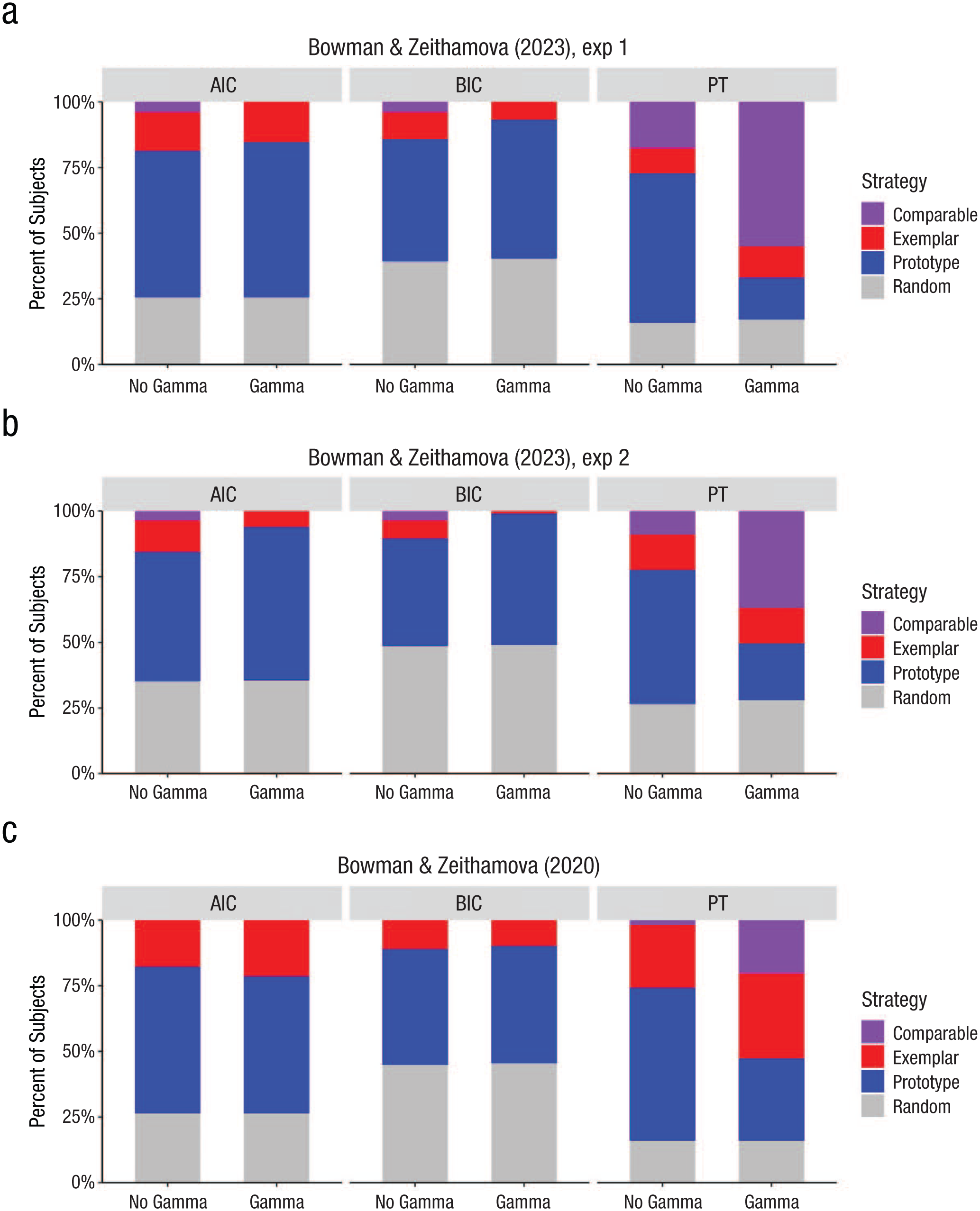
Strategy-assignment differences across different model-selection techniques. Each plot visualizes the proportion of subjects assigned a prototype strategy (blue), exemplar strategy (red), and comparable fit of both models (purple) and subjects not fit by either strategy better than chance (gray). (a) Experiment 1. (b) Experiment 2. (c) Bowman and Zeithamova (2020). The x-axis facet labels indicate which model-selection technique was used: Akaike information criterion (AIC), Bayesian information criterion BIC, or permutation testing (PT). The x-axis labels on the bottom indicate whether the prototype model was compared with a simple version of the exemplar model (no gamma) or a more complex exemplar model (gamma).

To provide an intuition why this may happen, consider a subject initially classified as an “exemplarist” under a simpler model who may no longer receive that label when a more complex version (e.g., one including a gamma parameter) is used. One practical issue is that optimization algorithms may struggle to find the best-fitting parameters in more complex models, particularly when parameters interact nonlinearly. In the exemplar model, for instance, the sensitivity parameter (c) and the response-scaling parameter (gamma) jointly influence behavior, making the optimization landscape more challenging.

Even when the best fit is achieved, the gamma-including model may still be penalized too heavily by AIC or BIC. As one example, consider a subject with perfect accuracy: Both prototype and exemplar models fit such data nearly perfectly, with negative log likelihood near zero. However, because the prototype model has fewer parameters compared with the gamma-including exemplar model, it will always be favored by AIC or BIC. The main issue is that AIC and BIC quantify model flexibility by its parameter count, with each extra parameter incurring the same penalty. But the gamma parameter may not add as much effective flexibility as the penalty implies because of its interaction with c. Both parameters influence how similarity is mapped to response probabilities, and in many cases, the c parameter alone can mimic the effects of gamma. For example, when c is high, the model can produce steep response gradients even without an explicit response-scaling parameter. As a result, the simpler model may approximate the performance of the more complex one but without incurring the penalty of an extra parameter.

This mismatch between penalization and actual flexibility can lead to underestimation of the more complex model’s value, resulting in more subjects being misclassified (e.g., as prototypists or random responders). In contrast, permutation-based approaches offer a more nuanced evaluation by empirically estimating the null distribution of model performance. This allows for a fairer assessment of whether the added parameter genuinely improves model fit without overpenalizing complexity.

Practice of Model Selection Using Permutation Testing

Setting a decision criterion

As we illustrated above, two models may not be equally flexible in practice even when they have the same number of parameters. It may not be valid to assume that a zero difference in model fits is the most appropriate cutoff point to determine which model fits better. Instead, a more precise approach is to compare the observed difference in model fits with the null distribution of the differences in model fits generated from the randomized data. Just like with comparison with chance, the advantage of the Monte Carlo approach is that one can directly quantify how likely or unlikely any fit difference is observed just by chance even if there was not real signal in the data. Model-fit differences unlikely to arise by chance are considered a strong indicator in favor of one model over the other. The challenge of establishing significance for a fit difference when comparing a nonnested model has long been known (Cox, 1962). Cox (1962) emphasized that differences in fits need to be considered in the context of their expected difference under null. He also demonstrated how this can be accomplished algebraically for comparing simple mathematical models, such as log-normal versus exponential-function fits. However, with more complex models, there are no established algebraic solutions ready to be applied, and deriving them de novo for every pair of models, every stimulus structure, and potentially every participant would be mathematically complex or impossible. As a standard numerical method, permutation testing provides a flexible and intuitive tool to empirically build such null distributions and conduct significance testing in any situation.

As with the comparison with chance, researchers have flexibility in what degree of evidence they deem sufficient to call one model a winner over the other. There is no right or wrong cutoff, and one may choose more stringent or more generous criteria depending on the goals. In an extreme case, one could use the same strict threshold as for comparison with chance and call only one model a winner if the fit difference is less than 5% likely to happen by chance. This may make sense in some cases when comparing simpler and complex models and when researchers need to guard against unnecessary complexity, essentially, when there are reasons to treat one model as the default or null model and another model as the model to be evaluated against it. We do not advocate for such a stringent threshold when comparing two models that are conceptually on similar footing, such as the prototype and exemplar models. If researchers are too reluctant to call one or the other model a winner, they may end up with a large proportion of ties, potentially limiting subsequent analyses involving the assigned strategy label. Thus, we typically adopt a more liberal threshold when comparing two cognitive models as a compromise between a strict alpha level of 5%—which could classify many subjects as showing comparable fits—and traditional no-alpha approaches that call a winner for any difference regardless whether the difference is meaningful or reliable.

The logic of using the null distribution of model-fit differences is illustrated in Figure 7a and is easily adaptable to any chosen cutoff probability values. Here, we consider the 75% of middle values (fit differences) from the null distribution too close to call because that is a criterion we used in several past studies (Bowman & Zeithamova, 2020, 2023, 2025; Houser et al., 2024). If the observed fit difference falls into this range, the subject would be labeled as having comparable model fits, with neither model clearly outperforming the other. When the observed fit difference falls among the 12.5% of most extreme negative values, we accept it as enough evidence that the exemplar model outperformed the prototype model, and the subject would be labeled as an exemplarist. If the observed fit difference falls among the top 12.5% of most extreme positive values, we accept it as enough evidence that the prototype model outperformed the exemplar model, and the subject would be labeled as a prototypist. For a representative subject from Experiment 1 depicted in Figure 7a, the observed raw fit difference was −6.42. The negative fit difference (exemplar – prototype) indicates smaller fit value (better fit) for the exemplar model. The probability of observing a fit difference as or more extreme is p = .0033 (one-tailed) because 33 out of 10,000 simulations resulted in such an extreme model-fit difference. We would thus confidently classify this participant as using an exemplar strategy.

Fig. 7.

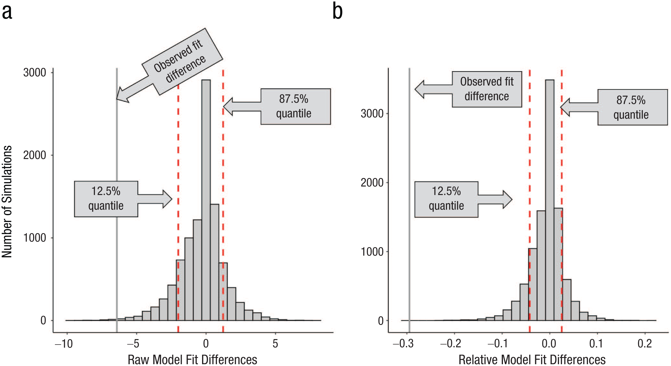
Decision criteria for model-fit differences. Distributions of model-fit differences for an example subject. (a) Raw model-fit differences, calculated by subtracting the prototype model fit from the exemplar model fit (exemplar – prototype). (b) Relative model-fit differences, calculated by dividing the raw model-fit differences by the sum of both model fits [(exemplar – prototype) / (exemplar + prototype)]. Vertical dotted red lines denote the 12.5% and 87.5% quantiles as examples of decision cutoffs. Solid vertical lines represent the empirically observed (left) raw or (right) relative model-fit difference.

Depending on the goals of a given study, it would also be reasonable to use even more liberal thresholds, such as considering just the 50% middle values to be ambiguous (just as likely than not to arise by chance) and values in the bottom quartile and the top quartile to be sufficient evidence to call one or the other model as a winner. Note that although setting the decision criterion is necessarily arbitrary, we argue that the Monte Carlo approach provides the advantage of being able to quantify the uncertainty of the decision. Furthermore, because the cutoff points are derived empirically, based on the Monte Carlo simulations rather than chosen arbitrarily and symmetrically around zero (for models with equal number of parameters), this approach accounts for potentially greater flexibility in one model that may not be reflected in the number of free parameters. Importantly, it works just as well for comparing models that differ in the number of parameters, allowing one to realistically account for the real flexibility the extra parameters afford.

Using the relative rather than absolute model-fit difference

Although the raw model-fit differences are informative, one of their disadvantages is that they scale with the overall fit values such that larger fit differences are more likely to arise by chance when the models’ fit values themselves are large. As a consequence, considering only raw model-fit differences could lead to overestimating the range of model-fit differences that can be observed just by chance when in fact, the range is narrower once the overall fit is taken into account. An alternative approach is to use the relative difference in model fits for model selection. The relative difference in fits is calculated as (exemplar model fit – prototype model fit) / (exemplar model fit + prototype model fit). Dividing the difference in fits by their sum results in fit differences as a proportion of the overall error in model fits. For example, a raw fit difference of 1 would be considered a larger difference if both models fit well (e.g., exemplar model fit error = 5.5, prototype model fit error = 4.5, 10% difference in fits) compared with when both models fit less well (e.g., exemplar model fit = 25.5, prototype model fit = 24.5, 2% difference in fits). Figure 7b illustrates the null distribution of the relative model-fit differences for the same subject as Figure 6a. As apparent from Figure 7, the observed fit difference is even more unlikely to arise by chance alone once we consider it in the context of the overall model fits. The observed relative fit difference was −0.29 (29% of the total fit). We found that the probability of the relative fit difference of this value or more extreme happening by chance is less than p < .0001 (one tailed) because zero out of 10,000 simulations resulted in such an extreme model-fit difference.

Using relative fit differences may be especially useful when the raw model fits leave too many subjects as appearing to have comparable fit just because large differences appear frequently by chance when fitting randomized data resulting in large fit values. Considering the relative fit differences also makes the values more comparable across studies (always scaled between −1 and +1) and less affected by external factors, such as the number of trials, that otherwise affect the raw fit values. However, in practice, the strategy assignments tend to be similar when using raw or relative model-fit differences (e.g., 97% match in Experiment 1 and 98% match in Experiment 2), and there are some challenges associated with using relative model fits, one of which we discuss in the following section. Thus, whether raw versus relative model fits are more suitable may differ between studies.

The special case of excellent fit by both models

Overall, we found the relative fit difference to be a practical and robust measure for model comparison and typically use this metric rather than raw model-fit differences. However, when both models provide an excellent fit, with negative-log-likelihood values near zero, the value of the denominator (exemplar + prototype) also ends up near zero. Because the fit values in commonly used software are never exactly zero, the calculation of the relative fit difference (exemplar − prototype) / (exemplar + prototype) does not trigger an explicit warning about dividing by zero and instead generates a large relative fit difference driven by the near-zero denominator. This then appears as strong evidence in favor of one model—when in fact, there are no fit differences and both models provide excellent fit. For example, one subject in our sample had prototype fit of 0.0000004 and exemplar fit of 0.0005. Such tiny deviation from zero is likely not meaningful; it may be a by-product of representation of small numbers in the particular software and/or noise in the fitting procedure. Nevertheless, if we were to compute the relative model fit without checking for such a scenario first, we would get an extremely large relative difference of 0.99, which never appears by chance when fitting randomly simulated responses. We would then confidently assign one or the other strategy to the subject even though both models have perfect fit and there is no way to decide between them for the particular subject.

Consequently, using the relative fit difference as a metric for model selection necessitates an extra step before model comparison: checking that the total model fit that serves as the denominator is not close to zero. In practice, we solve this problem by rounding the negative-log-likelihood fit values (e.g., to three decimal points) and then checking that at least one of them is different from zero. Only then would we compute the relative fit difference (which we do on nonrounded values or values rounded to five decimals). The relative model fits are problematic only when both models’ fits are near zero. In all other scenarios, including scenarios in which one model fits perfectly (near zero) but the other does not, the relative fit differences produce sensible values.

If both fit values are zero after rounding, we do not use the distribution of model fits but instead directly assign “comparable” (or “similar”) fit to a given subject because both models fit perfectly. Of course, the decision not to call a winner in these cases may not always be appropriate. We have used it when comparing prototype and exemplar models with equal numbers of parameters but also when comparing the prototype model with the more complex exemplar model with the additional gamma parameter (e.g., Bowman & Zeithamova, 2023). Because we are interested in the types of strategies people use and how they differ, we feel that not assigning a winning model in these cases is least likely to lead to erroneous conclusions. Nevertheless, AIC or BIC would in these cases automatically favor the simpler (in this case, prototype) model because it accounts for the data just as well while having fewer free parameters. Thus, when the number of subjects fit perfectly by both models is nonnegligible and the models do not have equal number of parameters, the decision how to call a winner when using relative fit differences may substantially influence the results and needs to be made carefully.

How many simulations does one need?

When using the Monte Carlo approach to model selection, how many random simulations does one actually need to estimate probabilities of a given effect to happen just by chance? Few cognitive-model-based studies perform model simulation (Palminteri et al., 2017), making it difficult to clearly define how many simulations are needed. One study investigated this question by evaluating 22 conducted studies across disciplines and found that researchers seldom provide justifications for the number of simulations they used (Mundform et al., 2011). Choosing 10,000 simulations has become relatively standard (Bicher et al., 2022; Heijungs, 2020; Koehler et al., 2009), which is what we have used in previous studies employing the same prototype and exemplar models discussed in the current article (Bowman et al., 2022; Bowman & Zeithamova, 2018, 2020, 2023). However, the simulations are needed for each subject and each model that is considered, which is more than 10 million simulations for this article. Each simulation is not just a single computation; instead, each of the 10 million simulations includes the use of an optimization algorithm that itself runs over many iterations. Thus, the compute time can potentially become a barrier to a wider adoption of these approaches. To overcome this challenge, here, we test the necessity of 10,000 simulations when determining generalization strategy via Monte Carlo procedures and demonstrate that fewer simulations are likely sufficient in most scenarios.

First, we consider the overall proportion of subjects relying on each strategy and how stable those estimates would be if fewer simulations were used. Considering 10,000 simulations as the “gold standard,” we compared differences in proportions of subjects receiving each strategy label (exemplar, prototype, comparable, random) if we were to use 100, 500, 1,000, 5,000, and 10,000 simulations. As visualized in Figure 8, the proportion of subjects from Bowman and Zeithamova (2023) receiving each strategy label is remarkably similar irrespective of the number of simulations.

Fig. 8.

Consistency of strategy labels across different number of simulations. Proportion of subjects from (left) Experiment 1 or (right) Experiment 2 that were assigned labels of prototypist (blue), exemplarist (red), comparable (purple), or random (gray) using null distributions comprising the number of simulations denoted along the x-axis. A gold rectangle outlines the strategy assignments when using 10,000 simulations because this is the “gold standard.”

Although the overall proportions changed little, we found several individual subjects whose strategy label would have been different had we used fewer simulations. Overall, we suggest that using 1,000 simulations is sufficient in most scenarios. First, we found that only five out 452 participants across both studies (1% of participants) would have received a different label if only the first 1,000 simulations rather than all 10,000 simulations were used. The overall 1% difference between 1,000 and 10,000 simulations appears like a modest gain for a tenfold larger computational cost. We also computed a standard test-retest reliability using 1,000 simulations and found 97.7% match in Experiment 1 and 99.3% match in Experiment 2 between the strategy assignment based on the first 1,000 simulations and the second 1,000 simulations. Of course, reliability will vary with the number of trials and other factors, and many researchers do not mind the extra computational cost to obtain the most stable answer. Nevertheless, we suggest that in many cases, using 1,000 simulations provides a reliable answer while substantially reducing computational cost.

Permutation testing and other goodness-of-fit criteria

Negative log likelihood is the standard goodness-of-fit measure when modeling categorical responses, such as trial-by-trial responses in categorization tasks. We generally favor fitting models at individual-subject level because group averages may not be representative of any one participant and may obscure the real processes underlying responses (Ashby et al., 1994). Nevertheless, there may be situations in which one needs to model continuous values from individual participants, such as reaction times, or continuous values obtained from group averages when modeling individual participants is not feasible. The most popular goodness-of-fit metric for fitting continuous data is root mean squared error (RMSE). Importantly, permutation testing is equally applicable in these situations. To test whether a model explains behavior better than chance (better than assuming no relationship between stimuli and responses), the obtained RMSE can be compared with the null distribution of RMSE values that can be obtained just by chance. To compare two models that may differ in content and/or complexity, the difference between two RMSE values can be compared with the difference expected just by chance. This again takes empirically into account the inherent flexibility of each model. To obtain the null distributions, individual subjects’ responses can be randomly permuted with respect to the stimuli, analyzed the same way as real data (e.g., averaged across participants followed by model fits into the group means), and the resulting simulated RMSE value stored. Comparison between the null distribution of RMSE values and the observed (empirical) RMSE value would follow the same logic as when negative log likelihood is used as the goodness-of-fit metric.

Other approaches to model selection

In this article, we focused on introducing model selection based on permutation testing, a hypothesis-testing tool widely used to establish significance when dealing with complex data (Berry et al., 2011; Good, 2000; Pesarin & Salmaso, 2010). All null hypothesis testing is based on the very same principle—estimating the probability that the data at hand could be observed just by chance if there was no real signal in the data (no differences between groups, no correlation between variables, etc.). In many circumstances, researchers do not have to run simulations and instead can use standard inference tests (t tests, analyses of variance, correlations). This is because under certain assumptions (independence, normality, etc.), the null distribution and the probability of each test statistic on that distribution has already been determined. Nevertheless, permutation testing provides a means to obtain the null distributions and p values in the broadest range of circumstances, including when there are no established test statistics to use.

Permutation testing is not the only proposed solution to some of the issues with traditional model selection. Most similar to permutation testing is bootstrapping (Buckland, 1998; Good, 2005; Mooney & Duval, 1993; Wehrens et al., 2000). Instead of permuting data to simulate the null distribution, bootstrapping focuses on estimating uncertainty by randomly sampling (with replacement) from observed data to estimate the sampling distribution. Essentially, it assumes that the observed sample is representative of the population and establishes the range of values one would expect to observe if one repeatedly ran many experiments drawing from this population. This allows researchers to estimate variability of performance metrics (negative log likelihood, RMSE, winning model, etc.) across resampled data sets. In the context of the current within-subjects model fitting, we can ask how stable a fit metric is or how stable (robust) the winning model is had the subject encountered a different random sample of stimuli. In other circumstances, we could ask how stable our findings would be had we collected a different sample of participants from the same distribution. Because the stimuli and the responses remain paired when using bootstrapping approach, bootstrapping may have one advantage to permutation testing for comparison of competing models. As discussed in the section on the use of relative model-fit differences, large model-fit differences can be observed just by chance when both models fit poorly (e.g., when fit to random data). Bootstrapping can help establish how robust the observed fit differences are within the region of space proximal to the real data. However, it does not resolve the problem of one model being possibly more flexible to fit any pattern of data. More complex resampling approaches have been proposed to tackle this challenge (Wagenmakers et al., 2004).

Another desired outcome of model fitting is finding a model that does not just fit the data at hand but also generalizes well out of sample. As noted above, AIC was developed with exactly this goal in mind: to select a model that would generalize and best predict future data. However, AIC penalization assumes large samples, and parameter-count-based approaches may fail when parameters have constraints or their effects are interdependent. One can overcome these challenges and test generalizability directly using cross-validation (e.g., Browne, 2000). In cross-validation, a model is fit into a portion of the data (referred to as “training data”), and the estimated parameters are then applied to the remaining data (referred to as “test data”). For example, here, we could fit a model into three-quarters of the trials (randomly selected) and test on the remaining one-quarter of trials. The model that predicts the unseen test data better would be considered a winner. Because the performance can be affected by the selection of the training and test data, we can repeat the procedure many times with new random training data/test data splits. This would generate information about not only which model wins more often but also how robust the model’s performance is, similar to the bootstrapping approach.

Finally, we discussed that BIC was developed with the goal of selecting a model that most likely gave rise to the data at hand. The BIC metric itself is a large-sample approximation, derived to estimate under certain assumptions the results of a more computationally complex model-comparison approach using Bayes’s factors (Heck et al., 2022; Kass & Raftery, 1995). Bayes’s factor compares two models by the ratio of their marginal likelihoods. Unlike the maximum-likelihood (best fit) methods discussed so far, marginal likelihood quantifies the probability of observing the data under a specific model considering (integrating over) the whole parameter space. This also means that model fits are not evaluated solely by their best-fitting parameters (as in maximum likelihood) but rather over the whole parameter space. This leads to an implicit penalty for model complexity: Although complex models have more flexibility to produce a pattern that matches the observed data well (better best fit), they also have more opportunity to produce patterns that are very different from the observed data, with the poor fits being averaged with the good fits for model evaluation (Lee & Vanpaemel, 2008). This computationally intensive approach to balancing fit with complexity is reminiscent of similarly implicit penalty for complexity in permutation testing, in which overly flexible models may have difficulty outperforming their own best fits to random data.

The Bayesian model-selection approach also allows one to specify what parameter values are a priori more likely. For example, instead of parameters being free to vary anywhere within their constrained or unconstrained range, one may assume based on prior research or theoretical considerations that they will be close to a particular value or follow a particular distribution. In addition to constraining models to avoid arbitrary complexity, this also makes it possible for more complex models to outperform simpler ones when an informative prior distribution reduces the impact of parameter values that may produce poor fits. For example, assuming that gamma is close to 1, the Bayes’s-factor approach can avoid overpenalization of the added gamma parameter (for a related discussion of the Bayesian approach of evaluating model complexity, see e.g., Shiffrin et al., 2008; Vanpaemel & Lee, 2012; Villarreal et al., 2023). The Bayesian framework also gave rise to two goodness-of-fit metrics, deviance information criterion (DIC; Spiegelhalter et al., 2002) and Watanabe-Akaike information criterion (WAIC; Watanabe, 2013). Unlike AIC and BIC, estimating DIC or WAIC metrics is computationally intensive, but especially WAIC is increasingly popular in hierarchical Bayesian modeling. Similar to AIC, WAIC is focused on prediction compared with BIC and Bayes’s factors that are focused on identifying the model that is the most plausible given the data.

Permutation-testing and Bayes’s-factors approaches can be viewed as largely complementary, similar to frequentist versus Bayesian approach to statistics more generally. Permutation testing focuses on constructing a null distribution to directly provide significance testing and p values for model comparison, similar to null hypothesis testing more broadly. Bayes’s factors focus on probability ratios (probability of data given each model) to generate the strengths of evidence (likelihood ratio) for one model over another, similar to Bayesian statistical approaches more broadly. Together with bootstrapping and cross-validation, these approaches use computationally intensive methods to go beyond assumption-heavy traditional metrics and provide robust means for model comparison and statistical inference in general.

Conclusions

In this article, we discuss permutation approach to model selection and demonstrate its benefits compared with more standard approaches, such as AIC or BIC goodness-of-fit criteria. We show that traditional penalization for free parameters may be too severe, especially when there are more parameters, constraints, and/or interdependencies. We further show that two models with equal number of parameters are not necessarily equally flexible and that one may fit better than the other just by chance. Because a model’s flexibility cannot always be discerned from its number of free parameters, challenging a key assumption in traditional model comparison, we demonstrate that permutation testing provides a more robust means for both comparison with chance and comparison between competing models. We conclude by discussing practical aspects of model selection using permutation testing, including setting of decision criteria, use of relative versus absolute model fits, and the number of simulations required to obtain reliable model selections at the individual level. Although permutation approach was once too computationally intensive for a wide adoption, it is now easily achievable on a personal computer while providing a robust means for model evaluation.