Handling Item-Level Missing Data in Linear Regression: A Tutorial

Abstract

With advances in methodology and statistical software, modern methods for handling missing data have become more accessible and straightforward to apply. In psychological studies, researchers often use questionnaires or scales composed of multiple items to measure constructs of interest. As a result, missing values frequently occur at the item level, whereas data analyses are typically conducted at the scale (composite) level. However, properly addressing item-level missing data remains a common challenge for many applied psychologists, including researchers who are otherwise well experienced in handling missing data at the scale level. In this tutorial, we introduce six approaches for handling item-level missing data: listwise deletion, hybrid methods that include proration with listwise deletion and proration with full-information maximum likelihood, item-level full-information maximum likelihood, item-level multiple imputation, two-stage maximum likelihood, and composite score factored regression. Using a published empirical data set, we provide step-by-step guidance on applying these methods in linear regression models. We include R code for each method and corresponding Mplus syntax if applicable. Finally, we summarize the key assumptions, advantages, and limitations of each approach and offer practical recommendations for researchers.

Item-level missingness is an inevitable problem in psychological research that uses multiitem questionnaires (Mazza et al., 2015). Typically, participants respond to items that make up various constructs, and these item-level responses are subsequently summed or averaged to generate scale-level composite scores. Missing data at the item level can occur for several reasons, such as participants refusing to answer uncomfortable questions or skipping those that they find inapplicable. In addition, planned-missingness designs are a common cause (Graham et al., 2006). Although handling the composite-score missingness (i.e., considering a scale-level score as missing when one or more of its items are missing) is an option, addressing item-level missing data is considered superior (Alacam et al., 2025) because it can use more information on within-scales covariation, thereby maximizing precision and power (Rombach et al., 2018; Savalei & Rhemtulla, 2017).

In empirical research, item-level missing-data handling is often poorly reported or incorrectly performed. Berchtold (2019) reviewed articles published in six top social-science journals in 2017 and found that more than half of the articles with item-level missing values did not clearly report the presence of missingness. Among those that did, most employed methods known to introduce bias estimates to address the missing values. This may be due to practitioners’ unfamiliarity with methods for handling item-level missing values. Although numerous methods exist to handle item-level missing data, the fragmentation of information makes it challenging for researchers to quickly and comprehensively understand these approaches. In addition, understanding the prerequisite assumptions and the applicable missing-data mechanisms required by each method presents further challenges.

In this tutorial, we aim to comprehensively summarize several existing approaches for handling item-level missing data: (a) deletion methods that include listwise deletion (LD), (b) hybrid methods that included proration with LD (P-LD) and proration with full-information maximum likelihood (P-FIML; FIML), (c) item-level FIML (IL-FIML), (d) item-level multiple imputation (IL-MI; MI), (e) two-stage maximum likelihood (TSML), and (f) composite-score-factored-regression (CSFR) method. For each method, we first introduce its key theoretical concepts and then provide and explain the software code for some key steps (complete codes are publicly available online). Finally, we present model results across different methods, summarizing the assumptions of each method, key advantages and limitations, and software availability. In the main text, we focus primarily on R software (R Development Core Team, 2022) code, but we also provide Mplus (Muthén & Muthén, 2017) code if applicable on OSF. The case scenario focuses on fitting data with item-level missingness to a scale-level multiple-linear-regression model because linear regression models are widely used and commonly applied in psychological research (e.g., Bjelland et al., 2008; Kovacs et al., 2009). Before proceeding, we assume that readers are familiar with linear regression models, path analysis in structure equation modeling (SEM), and R programming language.

Brief Data and Variable Description

To illustrate the application of different item-level missing-data-handling methods, we used a subset of data from a published study (Espino et al., 2023). The original data set included demographic variables and items assessing various psychological constructs from a sample of 1,276 Spanish students. For this tutorial, we focus on a multiple-regression model in which social support seeking (SS) is predicted by self-awareness (SA) and self-perceived peer support (PS):

$$SS={\mathrm{\beta }}_0+{\mathrm{\beta }}_1\left(SA\right)+{\mathrm{\beta }}_2(PS)+\mathrm{\epsilon }.$$

SS and PS are measured using four-item scales, and SA is measured by a five-item scale. The composite scale-level scores in this study are calculated as the mean of the item scores for each respective scale. ¹ To make the later discussion and code as general as possible, we define the SA as X, PS as Z, and SS as Y. Then, the regression model can be rewritten as follows:

$$Y={\mathrm{\beta }}_0+{\mathrm{\beta }}_{1}X+{\mathrm{\beta }}_{2}Z+\mathrm{\epsilon }.$$

(1)

There are missing values across all items in the subset, and the percentage of missingness is 17% (for the missingness pattern, see Fig. 1). ² For simplicity, the analysis is conducted on a randomly selected subset of 200 participants, focusing only on the relevant items. The used subset and complete R/Mplus syntax is available for download at https://osf.io/fy5ea. To help readers better understand the idea of subsequent code in this article, we display several rows of the data frame in Figure 2.

Fig. 1.

The pattern of missingness in the sample data set. The left column of values provides the missingness frequency of each pattern. The right column of values lists the number of missing variables per pattern. The bottom side of values provides the number of missingness per variable and the total number of missing cells.

Fig. 2.

Sample rows of the data set.

Approach 1: Deletion Methods

The oldest method to handle missing data is LD. LD, also known as “complete case analysis,” removes all cases with any missing items. Numerous studies have criticized the disadvantages of the LD method given it uses the smallest sample for analysis, leading to larger standard errors and lower statistical power (Fox-Wasylyshyn & El-Masri, 2005; Newman, 2014). Furthermore, LD relies on the assumption that the data are missing completely at random (MCAR), ³ which is generally considered an unrealistically strong assumption (Graham, 2009; Newman, 2014). We included this method in the article to provide a comprehensive comparison across approaches, particularly because it remains the default option in many statistical software packages unless specified otherwise, leading many practitioners to use it without awareness. However, we note that this method can introduce substantial bias and is widely discouraged in literature (e.g., Berchtold, 2019; Newman, 2014). Here, we use the mutate() function in the tidyverse package (Wickham et al., 2019) to compute the composite scores and the sem() function from the lavaan package (Rosseel, 2012) to perform the linear regression analysis.

We describe some key steps of the coding details below. First, we create three new scale-level variables (i.e., X, Z, and Y) by using rowMeans() function. By default (or by argument na.rm = FALSE), this function will calculate mean score of several items while treating the composite value as missing when there is at least one missing point. For example, if one individual has a missing value on one of the items for X, then the individual’s X scale value will be NA (Not Available).

Second, when fitting an SEM ⁴ model, the LD method can be employed either by specifying the argument missing = “listwise” or by default, in which case, observations with missing values on at least one composite score are excluded from the analysis (for codes, see Box 1).

Box 1.

Listwise Deletion

Approach 2: Hybrid Methods

When conducting scale-level analysis with item-level missing data, an alternative common approach is to combine different missing-data-handling methods. We begin with the proration method because it is the common component among the different hybrid methods. A prorated score, also known as “person mean imputation,” is calculated by replacing each participant’s missing-item scores on a scale with the mean of their available item scores on the same scale (Mazza et al., 2015; Wu et al., 2022). For example, if a person has a missing value for one item on the five-item SA scale, it will be replaced by the mean of the remaining four items for that individual. Although the proration method is recommended in some older user manuals, ⁵ it should be used with caution because it can yield highly biased estimates even under MCAR (Schafer & Graham, 2002).

Two hybrid approaches combined with proration include P-LD and P-FIML. P-LD combines proration method with scale-level LD, which can use more data information than item-level LD. P-FIML combines proration method with scale-level FIML (SL-FIML). SL-FIML is generally considered to be easy to conduct but can result in decreased power because of removing any incomplete cases and introducing biased estimates (more information about FIML will be provided in a later paragraph; Gottschall et al., 2012). Researchers believe that the combination of proration and SL-FIML may address their limitations; however, results show that it is unreliable under some missing mechanisms and sample-size conditions (Wu et al., 2022).

As before, we are using mutate() from tidyverse and sem() from lavaan for computing the composite scores and performing regression analysis, respectively. We describe some key steps of each approach below.

For each approach, we first generate averaged scale scores by using rowMeans() function with argument na.rm = TRUE. This argument will calculate the mean score for a scale using only available items for an individual. ⁶

Second, when fitting models, we use the argument missing = “listwise” or missing = “fiml” to apply LD or FIML methods, respectively (for codes, see Box 2 ). Note that P-LD removes an observation if any scale score is missing, whereas P-FIML excludes an observation only if all scale scores are missing. When some scale scores are missing, the available scores are still used in the scale-level FIML estimation process.

Box 2.

Proration With Listwise Deletion and Proration With Full-Information Maximum Likelihood

Approach 3: IL-FIML

FIML is one of the predominant methods in the context of SEM (Lee & Shi, 2021; Mazza et al., 2015). It does not rely on the MCAR assumption and requires only the weaker assumption that data are missing at random (MAR). FIML estimates model parameters by computing a likelihood function for each case using only the variables that are observed. ⁷ These individual likelihoods are then combined across all cases and maximized to obtain parameter estimates (Enders & Bandalos, 2001). When treating item-level missingness, a commonly used and straightforward strategy is to treat an individual’s composite score as missing when there is at least one missing item, which is referred to as “scale-level FIML” (Gottschall et al., 2012). Unlike deletion methods, SL-FIML retains the available scores from scale-level incomplete cases in the data analysis, enhancing the accuracy of the estimation (Mazza et al., 2015). However, this method still essentially performs deletion at the item level, which may lead to decreased power and biased estimates when item-level MAR is present (Gottschall et al., 2012).

To address the limitations of SL-FIML, Mazza et al. (2015) suggested using the IL-FIML approach, which combines all but one item from each scale as auxiliary variables in a saturated correlation model (Graham, 2003) and does not alter the interpretation of the coefficients. Like SL-FIML, IL-FIML first computes the composite scores, treating each score as missing when at least one item contains missingness. Next, it performs FIML to estimate the linear regression while incorporating some of the individual raw items as auxiliary variables. This means the raw item scores are added to the regression model and allowed to freely correlate with each other, the composite of the exogenous variable, and the regression residual. Although Mazza et al. found that including more items lead to better power, at most, k – 1 items can be included for each k-item scale to avoid linear dependency. They suggested omitting the item with the most concurrent missing rate with other items and in case of ties, to select the item less central to the scale construct. Note, however, that the inclusion of a large number of auxiliary items could drastically increase model complexity and lead to convergence issues. Because different exclusions of items being out of auxiliary variables can affect the parameter estimation, the subjective decision of selecting which variables can influence the results of the analysis.

We describe some key steps of the coding details below. First, we create scale-level variables by using the rowMeans() function with default argument (or by argument na.rm = FALSE) to calculate sum score of items while treating the composite value as missing when there is at least one missing point.

Second, when fitting models, the sem.auxiliary() function from the semTools package (Jorgensen et al., 2025) is employed to analyze data with FIML, using a saturated correlation model in conjunction with item-level auxiliary variables. The argument aux = c() is used to define a set of auxiliary items, including only k – 1 items for each scale. ⁸ The argument missing = “fiml” is used to link to the FIML method, and the argument fixed.x = F is used to treat all covariates as endogenous variables in the model (for codes, see Box 3). Note that multivariate normality is assumed for the covariates, and therefore, IL-FIML is not applicable to categorical variables. Treating categorical variables as continuous under this framework may result in biased parameter estimates (Enders, 2025).

Box 3.

Item-Level Full-Information Maximum Likelihood

Approach 4: IL-MI

MI is another common method for handling missing values, often compared with FIML. MI follows a three-step process: the imputation stage, the analysis stage, and the pooling stage. First, it creates multiple data sets by replacing missing values with simulated values based on the existing data and an imputation model. Next, the analysis model (in our case, the linear regression) is fitted to the multiple complete data sets. Finally, the estimated parameters and standard errors from the multiple data sets are pooled or aggregated into a single estimate and standard errors (Chen et al., 2020; Lee & Shi, 2021; Mazza et al., 2015).

IL-ML handles item-level missingness by including all items in the imputation phase before computing the scale scores (Savalei & Rhemtulla, 2017; Schafer & Graham, 2002). This approach maximizes the information used for imputations and significantly increases power compared with scale-level MI (Gottschall et al., 2012; Mazza et al., 2015). In addition, IL-MI tends to yield unbiased estimates under MCAR and MAR conditions (Newman, 2014) and typically yields the same results as FIML when the imputation model matches the FIML model and the number of imputations is sufficient (Lee & Shi, 2021). MI is also a flexible approach; for example, it can explicitly account for categorical items in the imputation process by specifying the appropriate imputation method. However, IL-MI can be challenging to implement for applied researchers because results can vary depending on the selection of the imputation model and the number of imputations. In addition, certain MI methods and a large number of imputations can lead to lengthy computation times. Moreover, repeated MI on the same data set may produce slightly different results each time (Chen et al., 2020).

We describe some key steps of the coding details below. First, in the imputation stage, the mice() function from the mice package (van Buuren & Groothuis-Oudshoorn, 2011) is used to generate MIs for missing data. We use the argument m = 100 to create 100 MIs. ¹⁰ The method = ‘pmm’ ¹¹ argument determines the imputation method. Note that this serves only as an illustrative example because alternative methods can be used depending on the type of data, for example, dichotomous or ordinal data (for details, see R script file on OSF). The seed = 98124 argument is included to ensure the reproducibility of our example. After imputation, it is important to assess the algorithm’s convergence. Ideally, the imputed values should remain free of trends as the iterations progress (for details, see R script file on OSF).

Second, in the analysis stage, the complete() function is used to extract the completed data sets in a specified format, ensuring that all 100 complete data sets are included in order. By setting action = “long” and include = TRUE, the new data set is formatted in a long structure, and the original incomplete data set is also retained. Next, scale-composite variables are generated by using the rowMeans() function with default argument. Then, the data set is converted back to the format used by the mice package using the as.mids() function. Finally, the regression model is fitted to each completed data set simultaneously by using the with() function.

Third, in the pooling stage, the pool() function is used to combine the estimates from each model, which produces a single consolidated set of estimated results (for codes, see Box 4).

Box 4.

Item-Level Multiple Imputation

Approach 5: TSML

A TSML approach was proposed by Savalei and Rhemtulla (2014) to address missing data in SEM parceling that was adapted for item-level missing data in linear regression (Chen et al., 2020). Similar to MI, TSML follows a two-step process. In the first stage, FIML is used to estimate a saturated means and covariances model at the item level, which is then transformed into the mean and covariance matrix of the corresponding scale scores. In the second stage, the desired model is fitted to the scale-level means and covariance matrices obtained from Stage 1 (Chen et al., 2020; Savalei & Rhemtulla, 2014). The original TSML approach provides a more flexible alternative to FIML and is considered applicable in any scenario involving missing data (Savalei & Bentler, 2009). It has been adapted to handle incomplete nonnormal data and extended to address item-level missing data (Savalei & Rhemtulla, 2017; Yuan & Bentler, 2000).

This two-stage item-level missing-data handling preserves all available item-level information and yields comparable performance with IL-MI (Chen et al., 2020; Mazza et al., 2015; Wu et al., 2022). It was also shown to be robust to dichotomous and four-categorical items despite lacking an explicit mechanism to handle categorical data. For simple regression, TSML can be performed using a Shiny app (Chen et al., 2020) with a user-friendly interface (for example and corresponding codes, see supplementary in OSF). In this tutorial, we use the R package twostage (Savalei, 2025) to facilitate TSML implementation for multiple regression, noting that this package is still under development.

We describe some key steps of the coding details below. First, we specify the model to be fitted. Next, we specify which items correspond to which composites. This step is optional, but it becomes especially helpful when working with a large number of items. To make the process more intuitive, we first rearrange the variables so that they follow the order of their corresponding composites in the model. For example, in the model Y ~ X + Z, we reorder the data frame so that the Y items come first, followed by the X items, and then the Z items. We then indicate the number of items in each composite using the rep() argument. Third, the stage0() function constructs a composite weight matrix C, determined by the mapping of items to their corresponding composites and the score type (here, we use type = 2 for averaged scale score ¹³ ). Finally, the twostage() function is used to estimate the model at the scale level using the C matrix obtained from the stage0() function (for codes, see Box 5).

Box 5.

Two-Stage Maximum Likelihood

Approach 6: CSFR

The factored regression is an advanced framework that has been gaining increasing attention (Enders, 2025). Although understanding of this method remains limited compared with traditional approaches, such as FIML and MI, it is recognized for its flexibility and is considered to provide compelling advantages (Alacam et al., 2025; Enders, 2025). FIML and traditional MI approaches (e.g., joint modeling, fully conditional specification) assume multivariate normality. However, categorical (e.g., gender, education) and ordinal (e.g., Likert-type) variables are common in psychological data; treating them as continuous may yield biased parameter estimates. Although categorical imputations can be handled with modern joint-modeling approaches using a latent-response framework, such methods often encounter convergence failures, particularly when the number of items is large (Alacam et al., 2025).

In contrast, factored regression acknowledges the multivariate structure without requiring researchers to explicitly specify it (Alacam et al., 2025; Enders, 2025). Consequently, it offers enhanced flexibility for accommodating complex analytical features, such as multilevel data structures and nonlinear relationships, and mixed data types (e.g., categorical and continuous variables, or skewed distributions; Enders, 2025). Alacam and colleagues (2025) further extended the factor regression with Bayesian estimation ¹⁴ to handle situations in which predictor and/or outcome variables are composite functions (CSFR). By constraining the between-scales regression slopes, CSFR helps mitigate both convergence issues and the “curse of dimensionality” that can arise in classical methods as the number of items or the proportion of missing data increases while maintaining accurate parameter estimates (Rombach et al., 2018; Wirth & Edwards, 2007). We refer readers to Alacam et al. for more technical details and a thorough discussion of this approach. Note that CSFR can also be adapted to handle missing-not-at-random mechanisms—the more flexible assumption and a common occurrence in real-world data (Du et al., 2022).

We describe some key steps of the coding details below. First, install the Blimp software, a free Mplus-like software for latent variable analysis with missing data that incorporates Bayesian estimation (Keller & Enders, 2023). Second, we create scale-level variables by using the rowMeans() function with default argument (or by argument na.rm = FALSE). Third, the rblimp() function from the rblimp package (Keller & Enders, 2023) is used to run the Bayesian factored-regression model. Fourth, by default, all incomplete item variables are treated as continuous. This choice is made for illustrative purposes and to ensure consistency with other approaches, recognizing that ordinal item variables can be easily specified using the ordinal argument (see the corresponding comment line in Box 6). Fifth, the model argument defines all factored-regression models. Specifically, the line “Y ~ (x1:+:x5)/5 (z1:+:z4)/4” represents the focal regression model, in which the outcome variable is modeled as a function of the predictor’s item-level variables and the :+: symbol constrains the individual predictor items to have the same slope. For instance, the (x1:+:x5)/5 means the outcome variable is predicted by the mean of items x1 to x5 ¹⁵ . The lines “x1:x5 ~ z1:+:z4” and “z1:z4 ~ 1” constructs the predictor-item regression models that link the items of predictors to each other, and the line “y1 y2 y4 ~ Y” generates the outcome-item regression models that link all but one items ¹⁶ of outcome variable to each other. ¹⁷ Finally, the seed = 98721 argument is included here to ensure the reproducibility of our example (for codes, see Box 6). Note that because a Bayesian method is used, checking the convergence of the Markov chain Monte Carlo algorithm is essential (for details, see R script file on OSF).

Box 6.

Composite Score Factored Regression

Summary

In this article, we present the theory, advantages, and disadvantages of six approaches for handling item-level missing values, includes LD, hybrid methods (i.e., P-LD and P-FIML), IL-FIML, IL-MI, TSML, and Bayesian factored regression specification. Empirical data are used as an example to demonstrate the application of these methods in R software based on a multiple-regression model. The aim is to offer readers who are already familiar with regression analysis and missing-value handling a comprehensive overview of these methods and to make their implementation more accessible to psychology practitioners. When fitting the model, different item-level missing-value-handling methods can lead to inconsistent parameter estimates. The estimation results for each method based on our example data are summarized in Table 1. In addition, because each method has its own assumptions regarding applicable missing-data mechanisms, advantages and limitations, and software compatibility, we summarize this information in Table 2 for readers’ quick reference. Based on the considerations outlined above and findings from previous simulation studies, we present the following recommendations for applied researchers addressing item-level missing data. We recognize that these recommendations are based on existing knowledge in this field and are therefore not exhaustive. We hope that future methodological research will continue to expand the evidence base, thereby enhancing practical guidance. Our specific recommendations are as follows.

Table 1.

Summary of Regression-Model Results Across Missing-Data-Handling Methods

Method	Used sample	Intercept	X		Z
			Slope(SE)	95% CI	Slope(SE)	95% CI
LD	166	−.129	.609 (.091)	[.430, .787]	.159 (.054)	[.052, .265]
P-LD	178	−.110	.593 (.089)	[.419, .767]	.164 (.053)	[.060, .267]
P-FIML	196	−.064	.561 (.090)	[.386, .737]	.171 (.055)	[.063, .278]
IL-FIML	196	−.031	.554 (.091)	[.376, .732]	.168 (.055)	[.059, .276]
IL-MI	196	−.019	.560 (.090)	[.383, .735]	.162 (.055)	[.054, .270]
TSML	196	−.045	.561 (.090)	[.384, .737]	.166 (.055)	[.058, .275]
CSFR	196	−.040	.558 (.094)	[.376, .743]	.167 (.056)	[.054, .277]

Note: LD = listwise deletion; P-LD = proration + listwise deletion; P-FIML = proration + full-information maximum likelihood; IL-FIML = item-level full-information maximum likelihood; IL-MI = item-level multiple imputation; TSML = two-stage maximum likelihood; CSFR = composite score factored regression; CI = confidence interval.

Table 2.

Assumption and Appliction Information for Each Missing-Data-Handling Method

Method	Valid for MAR	Advantage	Limitation	Software availability a
LD	No	Easy to understand	Biased under MAR Lower power in general	R/Mplus
P-LD	No	Easy to understand Better power than LD	Maybe biased even under MCAR Requires similar item-total correlations and high scale internal consistency reliability	R/Mplus
P-FIML	No	Relatively easy to use Performs better than LD and P-LD in simulation study	Complex proration cutoff Ad hoc approach with no theoretical guarantee of validity	R/Mplus
IL-FIML	Yes	Efficient and good coverage Easy to implement as structural equation model	Convergence issue with large model size Results can vary based on researcher decisions with auxiliary-variable selection.	R/Mplus
IL-MI	Yes	Efficient and good coverage Flexible advanced options available	Convergence issue with large model size Challenging to implement Results can vary based on researcher decisions during implementation. Results can vary based on the random seed.	R/Mplus
TSML	Yes	Efficient and good convergence No researcher decisions required	R package is still in early development.	R
CSFR	Yes	Flexibility for complex model and data Can be extended to deal with MNAR	Requires extensive knowledge Requires a separate software	R

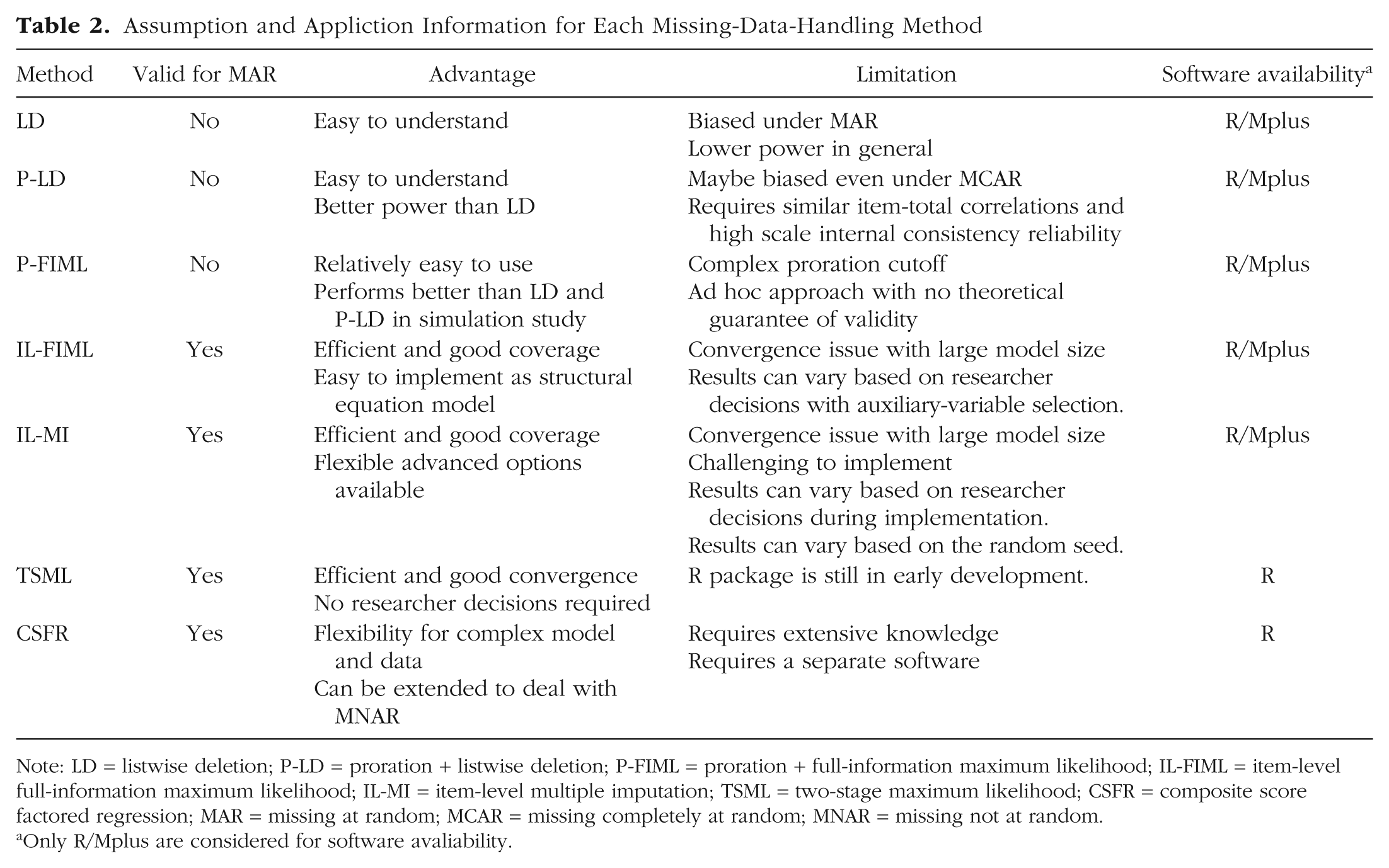
Note: LD = listwise deletion; P-LD = proration + listwise deletion; P-FIML = proration + full-information maximum likelihood; IL-FIML = item-level full-information maximum likelihood; IL-MI = item-level multiple imputation; TSML = two-stage maximum likelihood; CSFR = composite score factored regression; MAR = missing at random; MCAR = missing completely at random; MNAR = missing not at random.

a

Only R/Mplus are considered for software avaliability.

First, we recommend providing a detailed report on missing values. Rather than simply stating the overall proportion of missing data, specify how missingness is defined. In addition, report relevant information, such as the number of items with missing data and the percentage of missingness for each item. ¹⁸

Second, we strongly caution against using LD because it can produce biased estimates even under favorable conditions (Newman, 2014; Parent, 2013). SL-FIML may also yield biased results under MAR (Newman, 2014; Parent, 2013), and the P-LD method is similarly discouraged because it can be biased even under MCAR.

Third, for regression- and path-model analyses with a moderate sample size (at least N = 100), TSML provides a straightforward approach that requires no researcher decisions and yields comparable performance with other state-of-the-art approaches.

Fourth, IL-FIML and IL-MI methods are considered the “gold standard” (Enders, 2025; Lee & Shi, 2021). However, they involve some researcher decisions, and different researchers following the same analysis procedure can yield differing results, for example, selecting the inclusion of auxiliary items in IL-FIML and selecting different imputation methods or the number of imputations in IL-MI.

Fifth, when items are measured using Likert or Likert-type scales with a large number of response categories (i.e., five or more), ordinal data may be treated as continuous, which is the default setting for many item-level missing-data-handling techniques. However, when the number of response categories is small or when researchers prefer to treat the data as truly categorical, both IL-MI and CSFR can be readily implemented to accommodate categorical data with missingness.

Finally, when state-of-the-art approaches encounter convergence problems, it is essential to first ensure that the model is properly identified and not overly complex (Newsom et al., 2023). For FIML, increasing the number of iterations or modifying starting values may resolve nonconvergence. If item-level FIML or MI fails because of large model size, TSML or CSFR may be preferable because these methods generally exhibit fewer convergence issues given previous simulation studies (Alacam et al., 2025; Chen et al., 2020; Enders, 2025). P-FIML may also serve as an alternative, although it should be applied with caution.