
Abstract
The use of smartphones and wearable sensors to passively collect data on behavior has great potential for better understanding psychological well-being and mental disorders with minimal burden. However, there are important methodological challenges that may hinder the widespread adoption of these passive measures. A crucial one is the issue of timescale: The chosen temporal resolution for summarizing and analyzing the data may affect how results are interpreted. Despite its importance, the choice of temporal resolution is rarely justified. In this study, we aim to improve current standards for analyzing digital-phenotyping data by addressing the time-related decisions faced by researchers. For illustrative purposes, we use data from 10 students whose behavior (e.g., GPS, app usage) was recorded for 28 days through the Behapp application on their mobile phones. In parallel, the participants actively answered questionnaires on their phones about their mood several times a day. We provide a walk-through on how to study different timescales by doing individualized correlation analyses and random-forest prediction models. By doing so, we demonstrate how choosing different resolutions can lead to different conclusions. Therefore, we propose conducting a multiverse analysis to investigate the consequences of choosing different temporal resolutions. This will improve current standards for analyzing digital-phenotyping data and may help combat the replications crisis caused in part by researchers making implicit decisions.
In recent years, digital phenotyping has become increasingly popular in psychological research and is expected to transform health care and clinical practice (Huckvale et al., 2019; Jongs, 2021; Velozo et al., 2022). Digital phenotyping involves the “moment-by-moment quantification of the individual-level human phenotype in situ using data from personal digital devices” (Torous et al., 2016). Sensors on smartphones and wearable devices are used to passively collect data over time (Onnela, 2021). For instance, data on app usage, calls, text messages, GPS, Wi-Fi connection, and movement can be continuously captured throughout the day. Digital phenotyping has a low participant burden because it does not require active input from participants. Because most people have a smartphone, digital phenotyping is easily accessible to researchers (Luhmann, 2017).
To assess the feelings of participants that are not easily captured through passively collected data, digital phenotyping can be combined with “the experience-sampling-method” (ESM). In ESM, participants fill out brief questionnaires several times a day, for example, about their emotions (Kubey et al., 1996). This is typically done for several days or even weeks (Myin-Germeys et al., 2018). Digital phenotyping and ESM are increasingly used together in psychological research because they provide a powerful tool for capturing the daily life of a participant by measuring feelings and behavior (Rehg et al., 2017; Velozo et al., 2022).
Because digital phenotyping collects a large amount of data, additional methodological challenges are introduced when cleaning and analyzing such data (Barnett et al., 2018). These challenges often involve time-related decisions because data are collected almost continuously. All of these time-related decisions introduce many “researcher degrees of freedom,” or flexibility in analytical choices (Simmons et al., 2011). Currently, only a few studies have investigated the impact of specific temporal decisions (Bos et al., 2022; Cai et al., 2018; Heijmans et al., 2019). Those few studies suggest that the timescale at which passive measures are summarized and analyzed affects the outcome of the analyses. However, so far, there is little guidance or resources on how to choose a temporal resolution and how to analyze the data on different timescales (e.g., available R code). On top of that, no study has brought together these important time-related decisions.
In this article, we aim to improve current practices for analyzing digital-phenotyping data by discussing three time-related decisions that researchers face when summarizing and analyzing passive smartphone measures. We first introduce and explain these decisions and then perform a multiverse analysis taking them into account using data from 10 participants as an example. A multiverse analysis investigates how different plausible choices made by a researcher affect the conclusions drawn. Instead of doing an analysis only once, a multiverse analysis is done multiple times, including different plausible choices that a researcher can make (Steegen et al., 2016). We specifically focus on individualized analyses, which are commonly used in digital-phenotyping studies and are found to outperform nonindividualized prediction models (e.g., see Abdullah et al., 2016; Benoit et al., 2020; Cai et al., 2018; Davidson, 2022). However, these decisions are also important in nonindividualized analyses. Through our multiverse analysis, we show that time-related decisions can lead to different substantive conclusions. We end with recommendations for planning and conducting future studies that use digital phenotyping.
Data and Code Used for Illustration in Multiverse Analysis
Example data set and code
We provide an example data set (https://github.com/AnnaLangener/TimeScaleAnalysis_Example) and code (https://annalangener.github.io/TimeScaleAnalysis_Example/, written in R) other researchers can use as a starting point to explore different temporal decisions. For privacy reasons, we do not share the raw data of the participant but, rather, a data set with a similar structure and noise added. The full code used in this article is available in the GitHub repository (https://github.com/AnnaLangener/TimeScaleAnalysis).
Description of collected data
Throughout our article, we provide several illustrations to explain the time-related decisions faced by researchers when analyzing digital-phenotyping data. In these illustrations, we use data from 10 students from a Dutch university. Participants either received course credits or financial compensation for their participation in the study. In addition to other measures (e.g., social networks and interviews), participants filled out ESM questionnaires and installed an app that collected data passively for 28 days starting between October and December 2021.
ESM data were collected via the m-Path application (https://m-path.io), which participants installed on their own smartphones. Participants received push notifications for one semifixed morning questionnaire, four semirandom daily questionnaires, and one semifixed evening questionnaire. We removed the morning questionnaires from all of our analyses because people do not typically use their phones during the night. In addition, participants filled out questionnaires after each social interaction. Among other questions, the participants filled out three questions that measured momentary positive affect on an 11-point Likert scale (ranging from strongly disagree to strongly agree).
Alongside the ESM, participants installed Behapp (https://behapp.com) on their smartphones. Behapp collects data passively via the smartphone of the participant (Jagesar et al., 2021). In this study, we focus on the following sensors: GPS coordinates, calls, Wi-Fi scans, Bluetooth scans, and app usage. A full overview of all measures is provided in the following section.
Time-Related Decisions While Analyzing Passive Smartphone Measures
Temporal resolution while aggregating the data to create meaningful variables from raw passive smartphone measures
Background
Passive smartphone measures in their raw format are not very informative; instead, an extra step is needed first to create meaningful variables. For example, raw GPS coordinates (e.g., 50.8387326 and 7.0713267) are often measured to track individuals’ whereabouts, but by themselves, they do not provide much information about people’s behavior or how they spend their time. Therefore, researchers create meaningful variables by summarizing the raw GPS coordinates over a specific time window, such as the last hour or the last day. For instance, they may create variables that show how many unique places someone visited or how much time they spent at home during the last hour.
This also becomes relevant when merging data that capture different timescales. For example, passive smartphone measures are often measured almost continuously during the day, whereas ESM questionnaires are measured at only specific time points. Thus, to combine ESM and digital phenotyping, researchers have to choose a time window in which the passive measures are aggregated, for instance, before or after the ESM questionnaire was filled out (Velozo et al., 2022).
Different levels of temporal aggregation are used in the scientific literature to summarize passive measures, ranging from a few minutes to hours or even a full day (e.g., Chow et al., 2017; Kimhy et al., 2017; Stanislaus et al., 2020), and it is not evident which level of temporal aggregation is most appropriate. For example, some studies investigating the relationship between passive measures and social behavior have chosen to average the distance someone travels per day (Abdullah et al., 2016; Stanislaus et al., 2020), whereas other studies have done this per week (Fulford et al., 2021). Although both choices may be plausible, it is often left implicit which temporal resolution was used and why. As Wakim and colleagues (2020) noted, however, it is important to explicitly choose the level of temporal aggregation before data analysis is performed. Failure to do so can result in false-positive findings and difficulty in replicating the study’s results (Simmons et al., 2011; Wakim et al., 2020).
When choosing the level of temporal aggregation for digital-phenotyping data, it is important to consider the theoretical and conceptual basis for the decision. The chosen level of temporal aggregation should match the temporal resolution of the variables being studied (Cohen et al., 2020, 2021) and take into account how the variable of interest is expected to change over time (Haslbeck & Ryan, 2020; Wakim et al., 2020). For example, when studying Alzheimer’s disease, changes in behavior may occur more slowly and may be detectable on broader timescales (Wakim et al., 2020), such as weeks. In contrast, when studying mood, changes may occur more frequently and may be detectable only on shorter timescales, such as days or even hours (e.g., switching between depression and mania; Wilk & Hegerl, 2010). Theoretical and conceptual considerations can help justify the chosen level of temporal aggregation and ensure that it is appropriate for the variables being studied.
Likewise, when aggregating passive smartphone measures, researchers should first identify a specific research question and determine which concept they aim to measure. Conceptual clarity is critical in all psychological studies because poorly defined concepts make it challenging to build theories and interpret results (Bringmann et al., 2022). Nevertheless, there has been a lack of clarity regarding which construct passive smartphone measures aim to capture (Langener et al., 2023). For example, passive measures like GPS and accelerometer data are frequently used to measure social behavior; however, it is not yet clear which social behaviors these measures capture and how accurately these measures capture the intended construct (Langener et al., 2023; Tsapeli & Musolesi, 2015). Thus, researchers are advised to carefully consider the meaning of each variable they collect. This can be more beneficial than simply collecting as much data as possible and creating numerous features (Davidson, 2022).
It is also important to consider the meaning of the variables when measurements are summarized on different timescales because they may capture different behaviors and lead to different interpretations. For instance, using the same sensor and variable such as time spent at home, researchers can obtain insights into various types of behavior depending on the timescale chosen to process the data: GPS data aggregated over 24 hr can identify patterns in behavior across days, whereas a 1-hr time window can reveal a person’s circadian rhythm (W. Wang et al., 2018). Thus, researchers should consider the meaning of each variable (Borsboom et al., 2004), especially when measurements are summarized on different timescales, to ensure that the data captured reflect the behavior they intend to measure.
When theoretical considerations do not clearly dictate a particular level of temporal aggregation for digital-phenotyping data, researchers can use a multiverse analysis to assess the robustness of their results (Steegen et al., 2016). Cai and colleagues (2018) provided a good example of the use of a multiverse analysis in digital-phenotyping research. In their study, they used machine-learning models to investigate whether passive measures could predict momentary negative affect. They examined different levels of temporal aggregation for the passive measures, including the moment at which the ESM questionnaire was filled out and 1, 6, 12, and 24 hr prior. They found that the performance of the predictive models varied depending on the level of temporal aggregation used. Like Cai and colleagues, we illustrate how different levels of temporal aggregation affect the conclusions drawn. However, we first conduct descriptive and simple correlation analyses before moving on to more complex analyses, taking other time-related factors into account. This approach can help understand the robustness of research findings and ensure that they are not overly sensitive to specific choices made during data analysis.
Description of aggregated variables
We created several variables based on our raw passive smartphone measures. Some variables, such as minutes of calling, can be directly summarized into a variable in the aggregated data set referring to a specific temporal resolution (e.g., minutes of calling per hour). In contrast, other variables, such as GPS coordinates, require preprocessing steps even before they can be aggregated.
To calculate meaningful location features, one must make sense of recorded GPS coordinates. Therefore, before we aggregated GPS coordinates, we clustered them to “staypoints” (Zheng et al., 2009). This is based on previous work by Zheng and colleagues (2009). Based on the raw GPS coordinates, the algorithm returns a list of staypoints on which the participant has been stationary. A staypoint is defined as any location with a radius of 350 m where participants stayed for at least 30 min. Thus, strictly speaking, in this algorithm, a time window (i.e., 30 min) is chosen even before summarizing features to an aggregated data set. Because this choice is relatively arbitrary, it could also be part of a multiverse analysis. In our examples, we do not vary this time window because we focus on temporal resolutions to summarize and analyze all added variables and not on the time window chosen to calculate staypoints from GPS coordinates. The staypoint at which the participant spent most of the nights is labeled as the home location.
To add features about app usage, we classified to which category an app belongs. For instance, if someone uses WhatsApp or other messenger apps, we categorize them as communication apps. The categorization was done based on how an app is specified in the Google Play Store (Google Play Store Team, 2020). After doing those preprocessing steps we created our features referring to different temporal resolutions (1 hr, 3 hr, 6 hr, 8 hr, 12 hr, 24 hr). Table 1 provides an overview of the added features.
Overview of Data That We Use as an Example

Mac hash is a key that allows one to identify whether the same or a different phone number (has been) called or whether the same or a different Bluetooth/Wi-Fi connection was used while keeping the connection anonymous.
Example 1: preregistration of research question and hypotheses
In this article, we focus on the association between passive smartphone measures and momentary positive affect because the relationship between passive smartphone measures, health, and well-being is widely investigated (for a review, see Cornet & Holden, 2018). We argue throughout the article that it is important to preregister studies that use digital-phenotyping data to make those studies more reproducible. Therefore, we first describe our research question and hypotheses taking the level of temporal aggregation into account, which we would also do in a preregistration.
We start with investigating the relationship between the time spent at home and mood. Previous research indicated a positive association between the time spent at home and time being alone in control subjects (Fulford et al., 2021). In addition, Fulford and colleagues (2021) found that loneliness was associated with less time spent at home. On the basis of this evidence, we hypothesized a negative relationship between time spent at home and momentary positive affect because we expected that lonely people are less happy.
As a next step, we took previous research and theoretical considerations into account to formulate our hypotheses more precisely based on a particular timescale. On the basis of Fulford and colleagues (2021), we expected a negative relationship between time spent at home and momentary positive affect during the day. This is also in line with research suggesting that longer timescales can help to detect irregularities in an individual’s behavior, such as suddenly not leaving the house for an entire day (Cai et al., 2018). Our first research question and hypothesis are therefore as follows: 1
Research Question 1a: How is time spent at home during the day related to mood?
Hypothesis 1a: Time spent at home within the last 24 hr correlates negatively with momentary positive affect.
Current literature also suggests that mood fluctuates during the day and that longer timescales might not be suitable to capture those fluctuations (Kuppens & Verduyn, 2017). Thus, we expected that shorter timescales of aggregation (e.g., 1 hr before the ESM survey) may be more effective at capturing fluctuations in behavior that relate to mood. Thus, we investigated whether a negative association between time spent at home and mood exists over short timescales:
Research Question 1b: How is time spent at home during the last hour related to mood?
Hypothesis 1b: Time spent at home within the last hour correlates negatively with momentary positive affect.
We were additionally interested in the relationship between mood and minutes of calling. According to Duck and colleagues’ (1991) definition, phone calling qualifies as a social interaction if at least two individuals are engaged in the conversation and their behavior directly affects each other. Thus, phone calls can be seen as a form of social interaction. However, our measurement of phone calls included only direct phone conversations, and we did not account for calls made through messaging apps such as WhatsApp or other platforms. Thus, it is possible that some participants may have made additional phone calls that we did not capture in our analysis. Given the evidence that social isolation can negatively affect well-being (e.g., Ge et al., 2017; Teo et al., 2013), we expected that a higher duration of phone calls is associated with an increase in mood.
Phone calls are likely to occur infrequently throughout the day. Therefore, longer timescales, such as 24 hr, may be more effective in capturing their impact on mood because they may still have a significant effect. On the other hand, the impact on mood may decrease over time. For instance, a phone call that occurred 23 hr before the mood assessment may have less impact than one that occurred just an hour before. Thus, summarizing data over longer timescales risks including irrelevant information in each variable. Consequently, shorter timescales might be more suitable for measuring the direct impact on mood. As a result, we investigated the following research questions and hypotheses:
Research Question 2a: How are minutes of calling during the day related to mood?
Hypothesis 2a: Minutes of calling within the last 24 hr correlate positively with momentary positive affect.
Research Question 2b: How are minutes of calling during the last hour related to mood?
Hypothesis 2b: Minutes of calling within the last hour correlate positively with momentary positive affect.
In sum, we decided to investigate the association between momentary positive affect and passive smartphone measures (i.e., time spent at home and minutes of calling). On the basis of theoretical considerations and prior research, we chose to use a timescale of the entire day and the last hour before the ESM questionnaire being filled out. This is because these timescales have the potential to capture both short-term and long-term effects on mood. For instance, time spent at home or the number of phone calls made throughout the day may have a cumulative impact on mood, whereas the number of calls made within the last hour may reflect a more immediate effect on mood. However, we acknowledge that alternative timescales may also be relevant in measuring the impact of these passive smartphone measures on mood. To ensure the robustness of our findings, we employed a multiverse analysis that included temporal resolutions ranging from 1 hr to 24 hr, including 3-, 6-, 9-, and 12-hour intervals (as shown in Fig. 1).
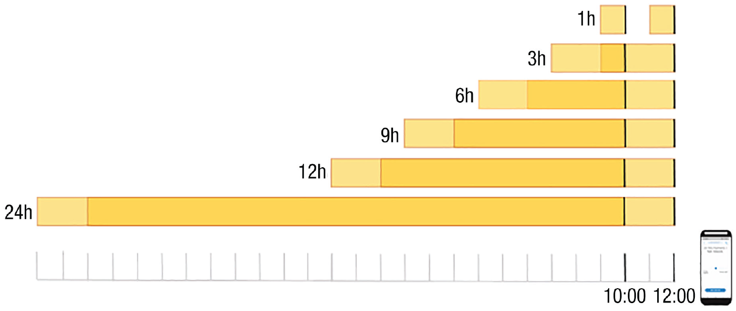
Digital-phenotyping data temporal aggregation. Shown are the six different temporal resolutions used in the analysis, including 1 hr, 3 hr, 6 hr, 9 hr, 12 hr, and 24 hr before an experience-sampling-method (ESM) survey was filled out (as indicated by the vertical black line, which indicates that the ESM survey was filled out at 10:00 a.m. and 12:00 p.m.). For larger levels of temporal aggregation, such as 3 hr, the data used to predict the outcome will overlap (as shown by the dark yellow part in the figure).
Results 1a: descriptive figures showing the variability of smartphone sensors
To better understand how the data varied over different timescales, we used line and violin plots to visualize the distribution of the data, which have been aggregated on different timescales (Hintze & Nelson, 1998). We used data from two individuals and two different passive measures. 2 To compare the variables aggregated over different timescales, we display them as percentages. For instance, 30 min spent at home would result in 50% of the time being spent at home using a 1-hr level of aggregation.
The first plot in Figure 2 shows the variation of the amount of time someone spent at home 1 hr before each ESM questionnaire was filled out. This means that the graph does not represent the raw passive measures but, rather, their aggregated version before each filled-out ESM questionnaire. For broader levels of temporal aggregation, the time spent at home before each ESM questionnaire seems to be relatively stable. For example, when aggregated over 24 hr, the minutes being at home seem to fluctuate between 70% and 100%, with an average of 88.9% and a relatively low standard deviation (SD = 15.9%). In contrast, when aggregated over shorter timescales, the time spent at home is more variable. For instance, using only the last hour before the ESM measures were filled out, the percentage of time spent at home is often either 0% or 100%, with an average of 68.3% and a relatively large standard deviation (SD = 44.5%). This makes sense because it is unlikely that an individual would switch between being at home and another location every hour. In contrast, over a longer time period, it is more likely that the individual would switch between being at home and another location. The important point is that the average value and variation of time spent at home differs depending on the level of temporal aggregation used. In this example, it is not clear which timescale is appropriate because there is no strong theoretical reason to choose one timescale over the other. As we show in Example 2, the chosen timescale will affect the analysis when we relate the minutes spent at home to another variable (e.g., mood).

Visualization of minutes spent at home (in percentage) aggregated on different timescales before the experience-sampling-method (ESM) survey was filled out (N = 99 ESM measurements). Shown are how the minutes spent at home (in percentage) evolve over time for different levels of temporal aggregation (top row). In addition, it illustrates the distribution of minutes spent at home using violin plots and the jittered raw data points next to them. Jittering involves adding random noise to the data, which slightly shifts the location of the data points. In our case, we added random noise on the horizontal axes. The depicted data are taken from one participant.
As another example, we investigated the minutes of calling on the phone before each ESM questionnaire was filled out (Fig. 3). The violin plots show that different levels of temporal aggregation capture different calls. For example, using a 1-hr level of aggregation, we found that the minutes of calling are nonzero for only four ESM measurements (M = 0.1, SD = 0.7), whereas broader timescales capture more minutes of calling (M = 0.13, SD = 0.36). One reason for this may be that using a lower level of temporal aggregation (e.g., 1 hr) may miss calls that happened between ESM measures, which are around 3 hr apart (e.g., if the call happened 2 hr before the ESM was filled out). In other words, if we use a lower level of temporal aggregation, we are not using all available data (see Fig. 1). In contrast, if we use a larger level of temporal aggregation (e.g., 24 hr), we are able to capture all calls because we use all available data. In addition, the data that we use overlap because our ESM questionnaires are around only 3 hr apart, whereas we always use the last 24 hr to aggregate our passive measures (see Fig. 1, dark yellow area). Therefore, in this specific example, using a too-short timescale may not capture enough calls, whereas longer timescales may be better because they use all the data between ESM questionnaires. This illustrates the importance of having a good understanding of the data, which can be done by visualizing the data on different timescales.
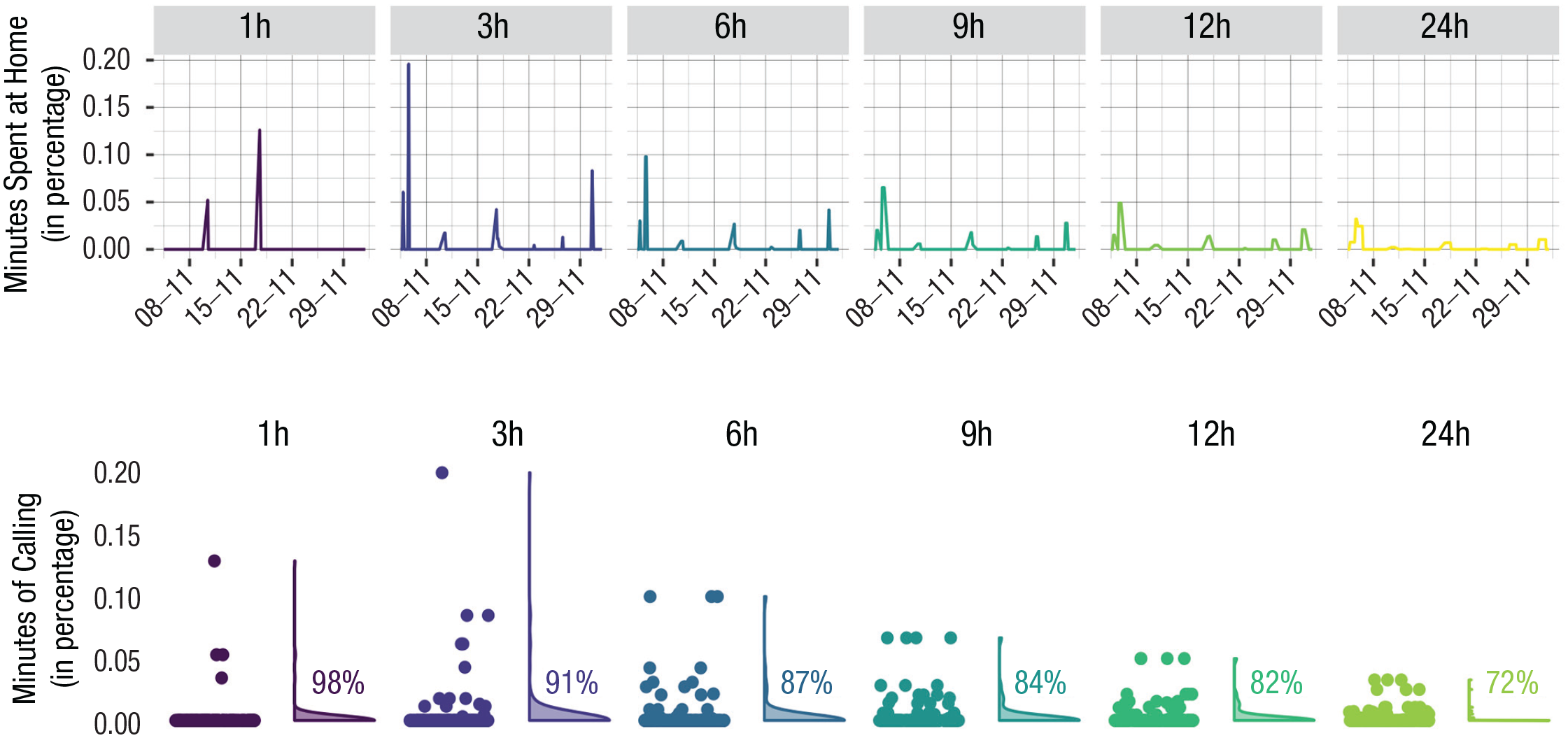
Visualization of minutes of calling (in percentage) aggregated on different timescales before the experience-sampling-method (ESM) survey was filled out (N = 163 ESM measurements). Shown are how the minutes of calling (in percentage) evolve over time for different levels of temporal aggregation (top row). In addition, it illustrates the distribution of minutes of calling using violin plots, with the jittered raw data points next to them. The percentages indicate the frequency of data points in which the minutes of calling were zero. The data are taken from one participant and demonstrate how aggregating passive smartphone measures at different timescales can affect the interpretation of the data. For example, if the measures are aggregated 1 hr before the ESM questionnaire was filled out, a point around 0.05 would indicate that the person was calling for 3 min (0.05 × 60). The same call would result in a much lower percentage for an aggregation level of 24 hr (0.002%).
Results 1b: using a different level of temporal aggregation to calculate the correlation between smartphone measures and momentary affect
To investigate the impact of choosing different timescales when analyzing the relationship between multiple variables, we calculated the bivariate correlation between passive smartphone measures and momentary positive affect. We aggregated the passive measures at various timescales. 3 To simplify the presentation of the results, we show correlations for only two individuals and two passive measures.
In our first example, we calculated the correlation between the total minutes spent at home and momentary positive affect for one participant including 99 ESM data points. The results show a significant negative relationship for relatively short timescales. This is in line with Hypothesis 1b, which suggested a negative relationship between time spent at home during the last hour and momentary positive affect. For instance, passive measures aggregated 1 hr before the ESM questionnaire was filled out led to a significant negative correlation of r = −.29, p < .01. Likewise, a 3-hr time span resulted in a correlation of r = −.26, p = .01. Contrary to Hypothesis 1a, this relationship becomes weaker and tends to zero over longer time spans (6 hr: r = −.15, p = .13; 9 hr: r = −.08, p = .45; 12 hr: r = −.01, p = .91). Note that even if not significant, the direction of the relationship changes for a 24-hr time span (r = .12, p = .24). This might be due to the reduced variability of minutes spent at home over longer time periods (see Fig. 2), which makes it more difficult to detect an effect (see Fig. 4). Alternatively, it might be because 24 hr is a too long time span to have an impact on mood. The key point is that different conclusions can be drawn depending on the chosen timescale, and this choice is not always justified by researchers.

Correlation between minutes being at home and momentary positive affect (for one participant) using different levels of temporal aggregation. The correlations are as follows: 1 hr: r = −.29, p < .01; 3 hr: r = −.26, p = .01; 6 hr: r = −.15, p = .13; 9 hr: r = −.08, p = .45; 12 hr: r = −.01, p = 0.91; 24 hr: r = 0.12, p = 0.24 (N = 99 experience-sampling-method survey measurements).
As a second example, we investigated the correlation between the total minutes of calling and momentary positive affect (see Fig. 5). For short time spans (1 hr, 3 hr) and a 24-hr time span, no significant relationship was found (1 hr: r = .07, p = .38; 3 hr: r = −.11, p = .15; 24 hr: r = −.09, p = .24; N = 163 ESM survey measurements). However, there is a significant correlation for medium-long time spans of 6 hr (r = −.16, p = .05), 9 hr (r = −.18, p = .02), and 12 hr (r = −.21, p = .01). Even if not significant, the direction of the relationship changes between 1 hr and longer time spans. This result is contrary to our Hypotheses 2a and 2b, which suggested a positive relationship between minutes of calling during the last hour and last 24 hr and momentary positive affect. A possible explanation for the different results of different timescales might be that most calls are not captured within short time periods (i.e., 1 hr and 3 hr) because the person does not frequently call throughout the day (see Fig. 3). Therefore, in this specific example, longer time spans can capture more calls and might be more informative. However, it might also be that we just found a spurious correlation for medium-long time spans.

Correlation between minutes of calling and momentary positive affect (for one participant) using different levels of temporal aggregation. The correlations are as follows: 1 hr: r = .07, p = 0.38; 3 hr: r = −.11, p = 0.15; 6 hr: r = −.16, p = .05; 9 hr: r = −.18, p = .02; 12 hr: r = −.21, p = .01; 24 hr: r = −.09, p = .24 (N = 163 experience-sampling-method survey measurements).
Both examples illustrate that the chosen temporal resolution can affect the results and conclusions drawn. Note that these examples are chosen to demonstrate how different temporal resolutions affect the robustness of results and therefore do not directly translate to other participants. The relationship between different passive measures and timescales varied among participants. We found that for most sensors and participants, the relationship between passive measures and momentary positive affect changed over different levels of temporal aggregation. However, participants and sensors differed in how the association changed (e.g., whether the association was significant and the direction of it). A full overview is available in the Supplemental Material available online (S1).
Handling missing data
Background
Missing data is another important factor that introduces researcher degrees of freedom. Missing data is important in all studies, but digital-phenotyping variables are particularly susceptible to missing data. Missing data can be random, for instance, when a phone battery died, an app crashed, or a Wi-Fi signal was lost. Nonrandom missing data might occur if the user actively turns off the permissions or the phone. Whereas random missing data is not related to the outcome variable, nonrandom missing data might correlate with the outcome of interest (De Angel et al., 2022; Onnela, 2021), for example, if the participant always turns off the phone while feeling sad, which can introduce biases in the results (Rubin, 1976).
Compared with most actively assessed data (i.e., questionnaires given to participants at specific time points), it is not always directly observable whether passively measured data are missing. 4 For example, a participant might not have used any apps throughout the day, so one would assume that the number of minutes the participant spent on apps was zero during that day. However, data on app usage could also be missing because of technical problems. For instance, data might be missing if the phone is turned off or the sensing app crashes (e.g., because of low battery; Barnett et al., 2018). Therefore, even if researchers start to monitor the reasons for missing data more closely, researchers do not always know whether a participant simply did not use apps or whether a participant used apps that were not recorded. This means that strategies must be chosen to exclude participants’ data.
In contrast to app usage, GPS coordinates are often recorded at fixed time intervals, so it is easily observable whether GPS data are missing. However, even for GPS data, it is important to choose a strategy to handle missing data. GPS coordinates are often used to compute staypoints, which are locations within a specific radius where participants stayed for a certain amount of time. During the study, the participant will likely lose the GPS signal for a certain time window. For example, the participant might go to a shopping mall, where they do not have a GPS signal for 2 hr (Zheng et al., 2009). After they are done shopping, the GPS signal is recorded again at the same location where they lost their signal previously. Consequently, the shopping mall would be clustered as a staypoint even if there are missing data in between. In this scenario, this would make sense and would create meaningful variables without missingness. However, it might also be the case that GPS data are missing for a longer time period or are recorded only sparsely throughout the day. In this scenario, the clustered staypoint might not change for several days, indicating that the participant did not move for several days, which is likely incorrect. Therefore, even for frequently recorded sensors such as GPS, it is important to choose a strategy to handle missing data to ensure acceptable data quality.
The rules for excluding participants’ data are often arbitrarily chosen, which can affect the reproducibility of research findings. For example, Yan and colleagues (2022) excluded a participant’s data for a day if all sensor data from that day were missing and assumed that their data were missing at random, whereas Nickels and colleagues (2021) included a day only if at least half a day of data from one frequently sampled sensor (e.g., GPS) was present and if the app measuring behavior passively was active for at least 18 hr of the day. Thus, studies differed in the measures they chose to exclude data and the time window of missing data they considered acceptable. Furthermore, systematic reviews have shown that missing data handling is often not reported, which can further hinder reproducibility (De Angel et al., 2022; Saccaro et al., 2021).
Results 1c: using different missing-data-handling strategies to calculate the correlation between smartphone measures and momentary affect
To evaluate the impact of missing data handling on the robustness of our results, we recalculated the correlations between being at home and momentary positive affect using different missing-data-handling strategies for a single participant. For simplicity, we used 1 hr of data aggregation before each ESM questionnaire was completed and did not vary the temporal aggregation strategy. We assumed that the data are missing at random and varied the time frame for identifying data as missing, such as excluding a day of data (i.e., clustered staypoints) if no GPS coordinates were recorded for 12 hr, 18 hr, or 24 hr during that day. We also varied which measures (e.g., app usage and GPS tracking) were used to identify missing data. For example, in one strategy, we would exclude GPS coordinates only if they were missing, although in another strategy, we would also exclude GPS coordinates if other frequently sampled measures (e.g., app usage, Wi-Fi, and Bluetooth) were missing even if GPS coordinates were present.
In our previous example, data were considered missing for a day if GPS data were missing for more than 24 hr, and the clustered staypoint was treated as missing for that day rather than assuming that the participant was not moving. However, other researchers have used more stringent criteria, such as excluding data for a day if app usage was not present for 12 hr on that day (e.g., Nickels et al., 2021). Applying these thresholds to our data, we found that using a 24-hr time frame for GPS data exclusion resulted in 17% of data being excluded, using an 18-hr time frame increased the exclusion to 22%, and a 12-hr time frame resulted in 31% of data being excluded (Fig. 6).
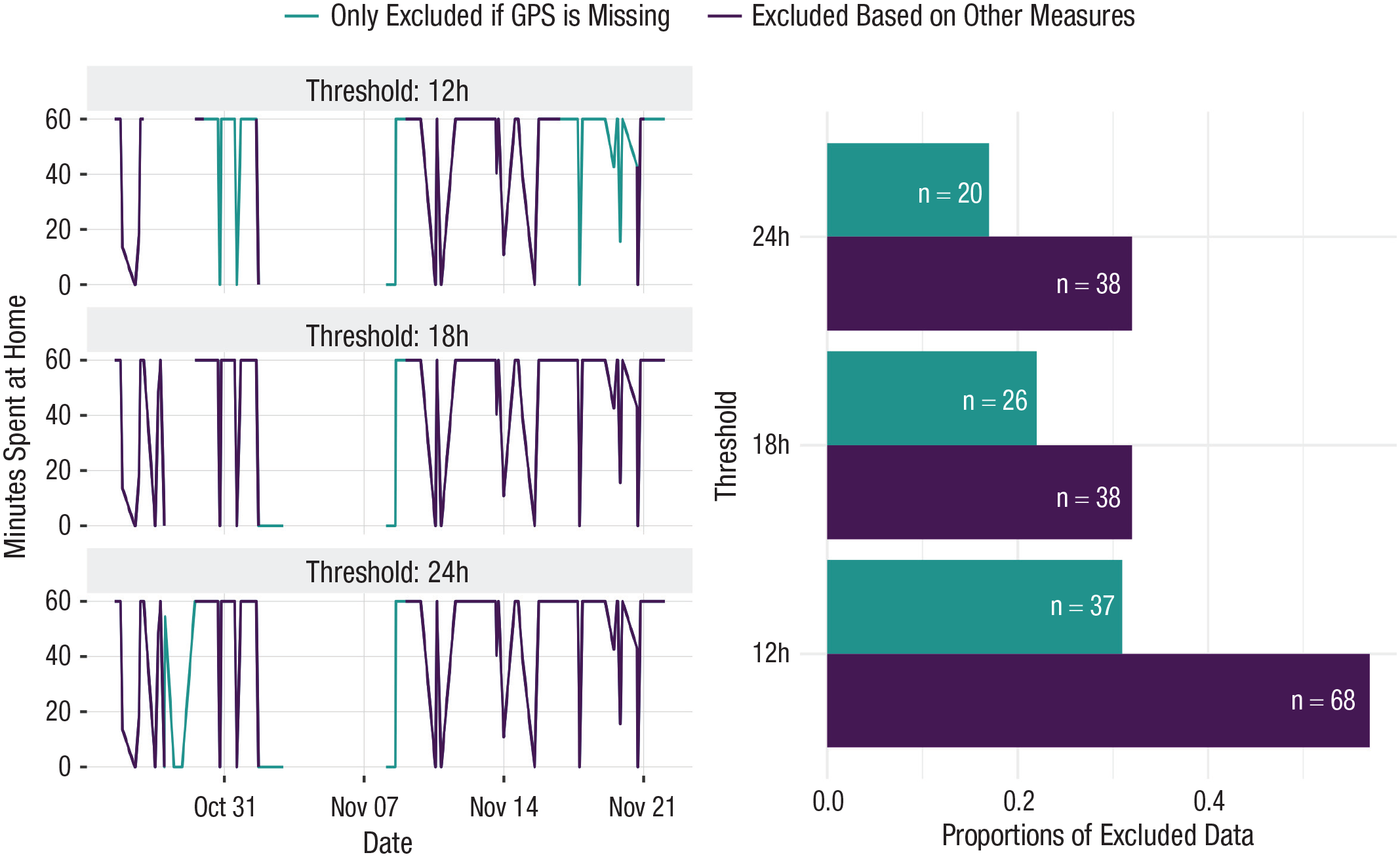
Proportions of excluded data using different missing-data-handling strategies. Shown is how much data gets excluded when using different missing-data-handling strategies. First, we varied the time frame that would lead to identifying data as missing (i.e., no data recorded for 12 hr, 18 hr, or 24 hr during the day). Second, we varied based on which measures the data were identified as missing (excluding GPS coordinates only if those are missing vs. also excluding GPS coordinates if other frequently sampled measures, e.g., app usage, Wi-Fi, or Bluetooth, are missing). Depending on which strategy is chosen, the number of excluded data points will change. We indicated above each bar how many experience-sampling-method (ESM) data points got excluded (e.g., n = 68 means that 68 ESM data points got excluded when using a threshold of 12 hr and excluding data based on several measures).
By examining how the correlation changes with different strategies that result in varying numbers of excluded data points, we found that using a 24-hr time frame for exclusion led to a significant correlation of r = −.29 (p < .01; N = 99; as reported in the previous section). Using a threshold of 18 hr resulted in the same association, whereas using a threshold of 12 hr resulted in a weaker correlation of r = −.19 (p = .09; N = 82). Therefore, using a frequentist approach to evaluate the correlation based on the p value, the conclusion drawn would be different for a 12-hr threshold compared with 18-hr and 24-hr thresholds.
An alternative strategy would be to exclude not only data from a particular measure (e.g., GPS) but also data from other measures within the same time frame because it is assumed that the data quality is low for that time frame (e.g., app usage, number of Wi-Fi connections; see Nickels et al., 2021; Yan et al., 2022). This results in an even more drastic reduction in data points: 24-hr and 18-hr time frames excluded 32% of all data points, and a 12-hr time frame excluded 57% of the data.
Recalculating the correlation using a 24-hr and 18-hr threshold would decrease the correlation to r = −.20 (p = .07; N = 81). Using a 12-hr threshold would result in a correlation of r = −.21 (p = .14; N = 51). We would therefore conclude that the data do not support a significant association between time spent at home and momentary positive affect.
Overall, it is clear that the threshold and strategies used for identifying missing data can significantly affect the number of data points that can be included in the analysis and, therefore, the statistical power. This is a significant issue in digital-phenotyping research because researchers often do not specify how to handle missing data (De Angel et al., 2022; Saccaro et al., 2021). When reported, it is evident that different strategies are often used (e.g., see different strategies used in Nickels et al., 2021; Yan et al., 2022), which is likely to affect the results.
Moving window while analyzing the data
Background
Many popular methods used in psychological research rely on running statistics over a specific moving time window, requiring researchers to actively choose the length of this time window (Scheffer et al., 2009; Wichers & Groot, 2016). For instance, to detect relapse in depression as early as possible, researchers might observe whether there is a change in the correlation between symptoms. To do this, they must choose a moving window in which to calculate the correlation.
Examining different window sizes can be a useful strategy in such cases to assess the stability of the results (Cabrieto et al., 2019). Bos and colleagues (2022) provided a positive example using a moving window to predict manic and depressive transitions in individuals with bipolar disorder and testing three different window sizes (1 week, 2 weeks, and 3 weeks). The results were largely robust, with only small differences found for different window sizes.
Finally, researchers often choose a particular moving window when performing more complex analyses. For example, researchers have started using passive smartphone measures to build individualized prediction models for mood and psychological symptoms (e.g., Abdullah et al., 2016; Jacobson & Bhattacharya, 2022; Jacobson & Chung, 2020). This is a promising field for developing just-in-time interventions (Balaskas et al., 2021; Jacobson & Chung, 2020). Just-in-time interventions are personalized interventions that are delivered to patients during daily life and may improve patient care in the future (Nahum-Shani et al., 2017). In addition, these methods, if successful, could potentially be used to replace or adapt daily questionnaires, reducing participants’ burden (Eisele et al., 2022; Hart et al., 2022). When using these prediction models, researchers commonly split the data into a training set (used to build the model) and a testing set (used to evaluate the prediction performance). To do this, researchers often choose a moving-window size, which can affect the prediction performance. For example, researchers might aggregate data at the hourly level and then use a rolling window of 24 hr to predict anxiety and depressive symptoms in the next hour (Jacobson & Bhattacharya, 2022; Jacobson & Chung, 2020). In our next example, we explore the impact of using different window sizes.
Example 2: preregistration of research question and hypotheses
In this example, we focus again on the association between passive smartphone measures and momentary positive affect. Our aim is to build a prediction model using passive smartphone measures. In this section, we describe our research question while taking time-related decisions into account.
Our broad research question focuses on whether we can predict momentary positive affect as a measure of current mood using passive smartphone measures, which is an important research question of the last decade (Cornet & Holden, 2018). To broadly capture an individual’s behavior, we used different passive smartphone measures as summarized in Table 1. We focused on two-time related decisions. First, we chose different temporal resolutions for aggregating the passive measures. Second, we chose different moving-window sizes in the cross-validation setup.
Similar to Jacobson and Chung (2020), we started by aggregating passive smartphone measures 1 hr before the ESM questionnaire was filled out. We think that 1 hr is a reasonable choice because it captures short-term fluctuations in the behavior of a person that might be linked to mood. However, in this example, there is no strong prior evidence to use one timescale over the other. Therefore, we also aggregated our passive measures on five additional timescales (i.e., see Figs. 2 and 3) to examine how stable our results are. Because this research is mainly exploratory and the main aim is to predict mood and not to understand a specific mechanism, no hypotheses were formulated. Our redefined research question is as follows:
Research Question 3: How well can we predict momentary positive affect using passive smartphone measures collected over the last hour, last 3 hr, last 6 hr, last 9 hr, last 12 hr, and last 24 hr?
In addition, we needed to choose the moving-window size for the cross-validation setup. To ensure transparency, it is essential to preregister the window size before analyzing the data. In our study, we varied the window size from six to 42 ESM measures, equivalent to approximately 1 day to 1 week of data, respectively. Our aim is to explore the impact of choosing different window sizes on the prediction performance. By exploring various levels of temporal aggregations and window lengths, we aim to gain insights into the optimal combination of a specific temporal granularity and trajectory length for accurately predicting positive affect. Thus, our last research question is as follows:
Research Question 4: Which combination of chosen level of temporal aggregation and moving-window size leads to the highest prediction performance?
Results 2: using a different level of temporal aggregation and a different moving window to predict momentary positive affect
In this illustration, we aimed to predict momentary positive affect (measured via ESM) using passive smartphone measures while examining two time-related decisions. We built an individualized prediction model using 185 ESM data points from 28 days. The participant used in this example did not have any missing passive smartphone measures.
To build a prediction model, it is standard practice to split the data into a training set and a test set. The training set is used to build the prediction model, whereas the test set is used to evaluate the prediction performance. Because we were using time-series data, it was important to take the order of the data into account when splitting the data into a training set and test set. In other words, it is important to consider the temporal direction, which means that researchers use only past data to predict momentary positive affect (Jacobson & Chung, 2020). A moving window cross-validation strategy can be used to take this temporal direction into account (Jacobson & Chung, 2020). This means that we trained the model on past observations (Fig. 7, training set, green squares) and used the trained model to predict the next observation (Fig. 7, testing set, purple squares). This process was repeated until the end of the data set was reached. The testing set consists of all predictions made across the different models (Fig. 7, purple squares).
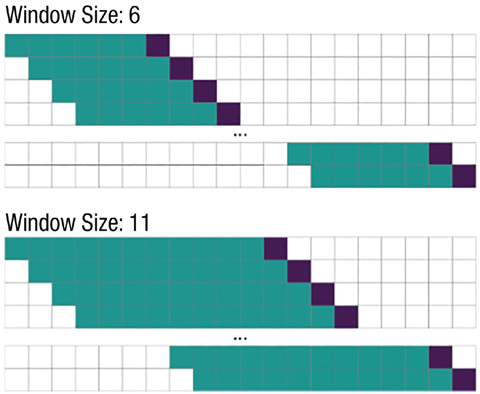
Example for moving window cross-validation setup. The upper part of the figure shows a moving-window size of six observations. This means that we build a model using only six observations as a training set, that is, six experience-sampling-method (ESM) questionnaires as an outcome and the corresponding aggregated passive measures as a predictor (green squares). This model was then used to predict the next observation, which was used as the test set (using the corresponding passive measures as predictors and the ESM questionnaire as an outcome; purple squares). The procedure was repeated until the end of the data set was reached. In contrast, the lower part of the figure illustrates a moving-window size of 11 training points. Likewise, the model is trained on the past 11 data points and used to predict the next point.
As previously mentioned, we had to choose the length of the moving window, which is another time-related decision that is likely to affect the results. For example, we might use the last six data points to train a model that is used to predict the next data point (see Fig. 7). In this illustration, we varied the moving-window size in the cross-validation setup that was used to predict momentary positive affect, ranging from six ESM measures (approximately 1 day of ESM measures) to 42 ESM measures (approximately 1 week of ESM measures).
We used random forest to predict momentary positive affect at a particular ESM survey using several passive measures. Random forest is a commonly used method in digital-phenotyping studies for predicting mental-health outcomes (e.g., for a review, see Benoit et al., 2020). We chose random forest because of its computational efficiency and ability to model nonlinear relationships (for more information on the algorithm and additional details, see the Appendix). Note that other models, such as simpler linear regression models or more complex models, could have also been used. The purpose of this illustration is not to assess the prediction accuracy of a specific machine-learning model or specific features but, rather, to compare the impact of temporal decisions on the robustness of the results in commonly used prediction models. In the remainder of this section, we discuss the impact of choosing different levels of temporal aggregation and the impact of choosing a different moving-window size, as summarized in Figure 8.

Individualized prediction model of momentary positive affect using passive smartphone data with different levels of temporal aggregation and different moving-window sizes. Shown is the explained variance for predicting momentary positive affect using only passive smartphone measures. The passive smartphone measures are aggregated on different levels, as shown by the different lines. In addition, we used different moving-window sizes in the cross-validation setup, which means that we varied the subset of data used to train the model, as displayed on the x-axis. For example, a 1-hr level of aggregation and a moving-window size of 20 would indicate that we aggregated the passive smartphone measures 1 hr before each experience-sampling-method (ESM) questionnaire was filled out and that we used a subset of 20 observations to build the prediction model. We compare this with using only the moving average of momentary affect as a prediction, without using any smartphone data. Here, a moving-window size of 20 would mean that we computed the mean of momentary positive affect over the last 20 ESM measures (yellow thick line).
First, we discuss the impact of choosing different levels of temporal aggregation of the passive data, which we used to predict momentary positive affect. Figure 8 displays the (out-of-sample) explained variance for different levels of temporal aggregation and different moving-window sizes in the cross-validation setup. The different levels of temporal aggregation are illustrated as the different lines in Figure 8. Overall, in this specific personalized-prediction model, broader levels of temporal aggregation perform better than lower levels of temporal aggregation. This means that on average, over all cross-validation setups (that used different moving-window sizes; see Fig. 7), most variance is explained with 24 hr of aggregation (M = 0.29, maximum = 0.33, minimum = 0.22), followed by 12 hr of aggregation (M = 0.28, maximum = 0.36, minimum = 0.22) and 9 hr of aggregation (M = 0.25, maximum = 0.37, minimum = 0.2). Consequently, lower levels of temporal aggregation lead to less explained variance (9 hr: M = 0.25, maximum = 0.37, minimum = 0.2; 6 hr: M = 0.23, maximum = 0.34, minimum = 0.15; 3 hr: M = 0.18, maximum = 0.28, minimum = 0.06); the least explained variance was for 1 hr of aggregation (M = 0.12, maximum = 0.28, minimum = −0.01).
Second, we discuss the impact of choosing different moving-window sizes of the cross-validation setup, which is displayed on the x-axis of Figure 8. The results indicate that the prediction performance gets worse if we include data points that were further in the past to train the model. Especially for lower levels of temporal aggregation (e.g., 1 hr of passive data before the ESM questionnaire was filled out), the explained variance reduces when choosing more data points to train the model (i.e., a larger moving window). Consequently, for 1 hr of aggregation and a moving window of six data points, the explained variance is 0.28 and decreases toward zero (R2 = .03) for using a moving window of 42 data points. For broader levels of temporal aggregation, the pattern seems to be similar but less extreme. Thus, within 24 hr of aggregation, a moving window of six leads to 0.33 explained variance, whereas a moving window of 42 leads to 0.28 explained variance. Overall, for this particular participant, a combination of a larger level of time granularity (temporal aggregation) and a shorter trajectory (moving window) yielded the best prediction performance for mood.
Choosing a smaller training window may yield superior results because momentary positive affect tends to vary less throughout the day compared with over a week for this specific individual. Using a smaller window size will therefore result in a lower range of possible values for positive affect, making it easier for the model to accurately predict mood. To investigate the impact of having a lower range of possible values for positive affect, we calculated the rolling mean of momentary positive affect for different window sizes. We use the rolling mean as a prediction to investigate whether using passive smartphone measures improves the prediction accuracy compared with solely using the rolling mean as the prediction. The results show that using passive measures increases prediction accuracy compared with using only the mean as a prediction. However, for very small window sizes combined with low levels of temporal aggregation (e.g., 1 hr and 3 hr of aggregated passive measures with a moving window smaller than 10), the moving average outperformed the predictions made using digital-phenotyping data. Overall, these results highlight the importance of considering temporal decisions when predicting mental-health outcomes using digital-phenotyping data.
Note that this example is based on only one participant. There was heterogeneity among participants in how well we were able to predict momentary positive affect. For some participants, it was not possible to give any acceptable prediction of momentary positive affect with the variables that we used. It also varied which level of temporal aggregation and which moving-window size led to the best prediction performance. Thus, those results do not directly translate to other participants. For example, for some participants, a larger moving-window size seemed to perform better (for an example, see S2 in the Supplemental Material).
Implications for Future Studies Using Digital Phenotyping
In our illustrations, we demonstrated that time-related decisions and strategies for handling missing data can significantly affect the conclusions drawn from the analysis, which further supports the results of previous literature (Bos et al., 2022; Cai et al., 2018; Heijmans et al., 2019). These findings have important implications for the design, analysis, and interpretation of future studies using digital-phenotyping data. In Table 2, we provide an overview of key decisions and factors to consider when choosing a specific timescale for aggregating and analyzing the data.
Overview of Important Decisions and Aspects to Consider While Choosing a Specific Timescale to Aggregate and Analyze Data

We recommend that researchers be explicit in their choice of temporal resolution when designing a study. This choice should be based on theoretical considerations and previous literature, and if multiple timescales are plausible, the researcher should consider conducting a multiverse analysis (Steegen et al., 2016) to explore associations on different timescales. If this is not feasible, researchers should clearly state that multiple timescales are plausible and explain the reasoning behind their choice of a specific timescale. It is important to consider the impact of temporal resolution on the results of a study given that our analysis showed that an association found at one resolution may not be present at another.
When choosing a specific level of temporal aggregation, it is important to consider how the variable of interest is expected to change over time. In our example, we aimed to predict mood based on passive smartphone measures. Research suggests that shorter timescales may be more suitable for predicting fluctuations in mood, such as the switch between depression and mania (Wilk & Hegerl, 2010). It may also be useful to consider how the passive measures are expected to change over time. For example, location data may change frequently, so shorter timescales may be appropriate. On the other hand, measures such as calling on the phone may change less often, so a longer timescale (e.g., a week) may be more suitable for detecting patterns. Checking and visualizing the digital-phenotyping data, as we did in Example 1, can be helpful for understanding how the passive measures fluctuate. When deciding on a specific level of temporal aggregation, it is also important to consider what each variable represents and how to interpret each variable taking the chosen level of temporal aggregation into account. In addition, it is important to consider how the chosen level of temporal aggregation aligns with the research question. For instance, when examining the direct impact of app usage on mood, a smaller level of temporal aggregation is more appropriate and better suited to capture the desired relationship.
For handling missing data, we recommend applying different strategies to ensure the robustness of the results. Once missing data are identified, researchers must also decide whether and how to impute the missing data. In our example, we did not impute missing data; however, depending on the research question, the analysis being conducted, and the variability of the measure, it can be beneficial to impute missing values (X. Wang et al., 2021). X. Wang and colleagues (2021) noted that GPS data require imputation to make sense of them. However, imputing missing data may be difficult if the measure is highly variable, and imputation could lead to decreased prediction accuracy (Nickels et al., 2021). Therefore, it is important for researchers to carefully consider whether to impute missing data or not and specify their decision beforehand. If missing data are imputed or deleted, researchers must carefully consider whether the chosen strategy assumes data are missing at random and whether this assumption holds in their specific study context.
The choice of moving-window size is important in considering how the association of interest is likely to change over time. Shorter moving-window sizes can capture changes more effectively and are useful for short-term predictions, such as for just-in-time interventions. On the other hand, if the goal is to make longer-term predictions and build a more robust prediction model, a larger time window may be necessary. Further research is needed to determine the optimal moving-window size for various applications (see also H. Wang et al., 2020).
Regardless of what the researcher decides, those choices should preferably be stated in a preregistration. This goes in line with previous recommendations about making researchers’ decisions explicit beforehand (Simmons et al., 2011). Choosing a level of temporal aggregation is similar to specifying in advance how a particular variable will be constructed. Likewise, choosing a time window for analysis is akin to stating in a preregistration which statistical method will be used, which can help to increase the robustness of the results (Chambers, 2013; Nosek & Lakens, 2014; Wagenmakers et al., 2012). Therefore, when using digital phenotyping, we recommend applying some of the same standards already in place for other psychological studies.
When writing up an article using digital-phenotyping data, it is important for researchers to explicitly discuss previous studies that have investigated the association of interest and be transparent about the timescale used in those studies. In addition, the preprocessing and data-cleaning steps taken should be clearly described. This transparency should be maintained throughout the article, including in the presentation of hypotheses and the interpretation of results, which should be based on the chosen timescale.
Discussion
Passive smartphone measures provide a valuable opportunity to track individuals over time and are increasingly used in psychological research (Onnela & Rauch, 2016; Perez-Pozuelo et al., 2021; Torous et al., 2016). However, these measures also introduce numerous researcher degrees of freedom that may not be reported transparently (Onnela, 2021). In this article, we emphasized the time-related decisions that researchers must make when analyzing digital-phenotyping data. These include choosing temporal resolutions to summarize collected variables, such as how much time someone spends at home per day or how many calls someone makes in the last hour. In addition, researchers must decide how to handle missing data and choose a specific time frame for various analysis techniques. Finally, we provided considerations, recommendations, and resources (i.e., available R code) for future studies that use digital-phenotyping data (summarized in Table 2).
We used multiple examples to demonstrate how the use of different timescales and strategies for handling missing data can affect the results and lead to different conclusions, which was also shown in a few previous studies (Bos et al., 2022; Cai et al., 2018; Heijmans et al., 2019). In our final example, we used an individualized prediction model to examine the impact of different moving-window sizes in the cross-validation setup and also varied the level of temporal aggregation of the passive measures. Individualized prediction models offer great potential to improve patient care through just-in-time interventions (e.g., Abdullah et al., 2016; Jacobson & Bhattacharya, 2022; Jacobson & Chung, 2020). Our results showed that both the level of temporal aggregation and moving-window size had a major impact on prediction performance.
Limitations and future outlook
In this article, we highlight the importance of selecting an appropriate timescale when analyzing passive smartphone measures. This challenge is not unique to digital-phenotyping studies because other fields working with sensor data face similar challenges. For example, in studies involving raw EEG or EKG signals, time windows are chosen to split the data into epochs, which are then used to calculate so called time-domain features such as the mean or standard deviation. Previous research highlights that the chosen epoch length can affect the relationship to the outcome measure (Bonita et al., 2014; Fraschini et al., 2016; Gudmundsson et al., 2007; van Diessen et al., 2015). Therefore, ideally, the length should be informed by theoretical assumptions. For example, a study that investigated the relationship between fetal heart rate variability and fetal distress chose a shorter time interval because newborns have a higher heart rate than children or adolescents (Govindan et al., 2019). For digital-phenotyping studies, it would be valuable to also conduct studies that test a specific level of temporal aggregation based on theoretical assumptions for a specific sensor and research question.
Likewise, functional MRI studies also use a specific time window to process their raw data. We can learn from those studies that it can be beneficial to use variable time windows in which variables are calculated. For example, for studies that investigate attention or decision-making, the response time of the participant to a particular stimulus can be used as a time window to create features. This can provide a more accurate picture of decision-related cognitive processes (Grinband et al., 2008). It would be interesting to investigate whether variable methods to aggregate features could also be useful for digital-phenotyping studies.
In cases in which no clear theoretical preference exists for a specific timescale, determining the optimal level of temporal aggregation and moving-window size during the hyperparameter tuning can enhance practical applicability and mitigate overfitting risks. Treating these choices as hyperparameters enables the selection of optimal values within the training set rather than retrospectively determining the timescale (Yang & Shami, 2020). In addition, employing Bayesian stacking, a technique that combines predictions from multiple models with different moving windows using a weighted average, might further improve prediction accuracy (Yao et al., 2022).
Throughout the article, we argue that researchers need to choose a level of temporal aggregation to summarize their data collected using passive smartphone measures. However, there are some exceptions in which it may be possible to use nonaggregated data sets, such as in deep-learning models and statistical models that explicitly model time, such as long short-term memory networks and proportional-hazard models (for more details, see Allison, 2014).
We highlight that different levels of temporal aggregation may be most suitable and necessary for different sensors (e.g., calls vs. GPS) and individuals. In our example, we conducted the same analysis several times using various timescales. However, for some applications, it may also be beneficial to combine sensors aggregated over different timescales into a single analysis. When doing so, it is crucial to consider the different chosen timescales while interpreting the results of each predictor. It is also possible to add the same sensor, aggregated over different timescales, to the (machine learning) model. Sano and colleagues (2018), for example, aggregated data from their sensors over a day and over different time intervals throughout the day to predict stress and poor mental health. Their results showed that the most important features to predict stress and low mental health were a combination of features that were aggregated over different timescales (e.g., skin conductance was aggregated between 9 a.m. and 6 p.m., and screen time was aggregated between 00:00 and 24:00). Adding aggregated data from the same sensor over various timescales will result in a large number of variables. Therefore, it is essential to select a modeling strategy capable of handling a large number of predictors (e.g., lasso regression; Tibshirani, 1996).
To account for the heterogeneity of the optimal timescale between individuals, hierarchical or multilevel models can be applied. For example, random slopes can be added to predictor variables that are aggregated over different timescales. This allows the effect of each predictor to vary across individuals (Brown, 2021). Another option is to combine individualized and nonindividualized machine-learning models. For example, Jacobson and Chung (2020) added the predictions of a nonindividualized machine-learning model as a variable to the individualized machine-learning models. This allows modeling differences within and between people. To get more insights into those differences, feature-importance scores can be calculated.
Another important method to process passive smartphone measures is to summarize variables from several sensors into a single score. This methodology is comparable with using questionnaires that measure the same construct with several variables. To summarize these variables, sum scores are often calculated or factor analysis is used, which broadly falls under the latent-variable framework (McNeish & Wolf, 2020). For example, in our study, we used several items to measure momentary positive affect. Likewise, researchers using passive smartphone measures have begun to define constructs that are measured by several sensors. For example, Eskes and colleagues (2016) calculated a sociability score consisting of various passive measures (e.g., calling behavior, Bluetooth density, and GPS data). When calculating such a score, it is again important to clearly define the construct and to take the chosen level of temporal aggregation into account.
We addressed three important decisions related to time in the context of digital phenotyping: summarizing the data, handling missing data, and data analysis. However, there are other time-related decisions that are important to consider in the research process. For example, before collecting any data, researchers must choose a sampling scheme, such as how often GPS coordinates are collected, to avoid draining the device’s battery (Torous et al., 2018; Velozo et al., 2022). Researchers also need to decide on the duration of the study. Although these decisions are important, we did not address them in this article because our focus was on data cleaning and analysis.
Although we mentioned options for dealing with missing data, there are other important strategies that are less related to time but still relevant for the analysis of digital-phenotyping data. One method that is increasingly being used is to create data-quality indices and include these indices as covariates in the analysis (Torous et al., 2018). For example, a data-quality index could be a variable that indicates the ratio of observed data compared with expected data. Torous and colleagues (2018) found that these indices are associated with several outcome variables. For example, an increased amount of recorded GPS data was associated with higher scores in clinical outcomes, such as anxiety and psychotic symptoms.
While using passive smartphone measures in research, researchers must make other decisions that are not directly related to time but can still introduce researchers’ degrees of freedom. For example, there are various algorithms and methods for clustering location data (examples described in Müller et al., 2022; Zheng et al., 2009), and researchers must decide which one to use to cluster the staypoints.
Overall, there are many decisions that researchers must make when working with passive smartphone measures, and we propose that future research should be more explicit about these choices. To improve transparency, researchers could consider using a preregistration template for digital-phenotyping studies, using our suggestions here as a basis, similar to those used in ESM studies (e.g., preregistration template for ESM studies; Kirtley et al., 2018). This would help make researcher degrees of freedom explicit and improve the transparency of digital-phenotyping research.
Throughout the article, we emphasize the importance of doing a multiverse analysis to enhance the robustness of our results. Although we provide a straightforward example of comparing outcomes according to different decisions, there exist more complex approaches to interpreting and presenting the results derived from a multiverse analysis. One such approach, which can be applied when using a frequentist framework, involves generating histograms of the derived p values. This enables an investigation into the stability of the results and the influence of various choices on the outcome (Steegen et al., 2016). Another approach would be to use a specification-curve analysis to show the strength of association across different possible decisions (Simonsohn et al., 2020). For example, by calculating the median effect across all decisions (for more information on conducting a specification-curve analysis, see Simonsohn et al., 2020). Recently, a tool became available that can help researchers facilitating the execution of a multiverse analysis (Liu et al., 2021). We recommend researchers to explore these different approaches of doing a multiverse analysis to select the most appropriate method.
In our example, we aimed to predict momentary positive affect measured with several self-reported questions. A major drawback of self-reported mood is that collecting such data is burdensome to the participant, which might have negative effects on the validity of the data (Asselbergs et al., 2016). This, in turn, could affect the association between mood and passive smartphone measures and the performance of the prediction models.
Conclusion
Digital phenotyping is a valuable tool for psychological research and is becoming more widely used. However, we demonstrated through various examples that the timescale on which digital-phenotyping data is summarized and analyzed can lead to significantly different conclusions. To improve current standards for analyzing these data, we recommend that researchers carefully consider the appropriate timescale when designing a study and interpreting the results. We also suggest conducting a multiverse analysis to investigate the effects of different temporal resolutions. Overall, we believe that these efforts are necessary to improve the replicability of studies using passive smartphone measures.
Supplemental Material
sj-docx-1-amp-10.1177_25152459231202677 – Supplemental material for It’s All About Timing: Exploring Different Temporal Resolutions for Analyzing Digital-Phenotyping Data
Supplemental material, sj-docx-1-amp-10.1177_25152459231202677 for It’s All About Timing: Exploring Different Temporal Resolutions for Analyzing Digital-Phenotyping Data by Anna M. Langener, Gert Stulp, Nicholas C. Jacobson, Andrea Costanzo, Raj R. Jagesar, Martien J. Kas and Laura F. Bringmann in Advances in Methods and Practices in Psychological Science
Footnotes
Appendix
Acknowledgements
The funding provider had no role in the study design, collection, analysis, or interpretation of the data, writing the manuscript, or the decision to submit the paper for publication.
Transparency
Action Editor: David A. Sbarra
Editor: David A. Sbarra
Author Contribution(s)
ORCID iDs
Notes
References
Supplementary Material
Please find the following supplemental material available below.
For Open Access articles published under a Creative Commons License, all supplemental material carries the same license as the article it is associated with.
For non-Open Access articles published, all supplemental material carries a non-exclusive license, and permission requests for re-use of supplemental material or any part of supplemental material shall be sent directly to the copyright owner as specified in the copyright notice associated with the article.