
Abstract
In recent years, machine learning has propagated into different aspects of psychological research, and supervised machine-learning methods have increasingly been used as a tool for predicting human behavior or psychological characteristics when there is a large number of possible predictors. However, researchers often face practical challenges when using machine-learning methods on psychological data. In this article, we identify and discuss four key challenges that often arise when applying machine learning to data collected for psychological research. The four challenge areas cover (a) limited sample size, (b) measurement error, (c) nonindependent data, and (d) missing data. Such challenges are extensively discussed in the “traditional” statistical literature but are often not explicitly addressed, or at least not to the same extent, in the applied-machine-learning community. We present how each of these challenges is dealt with first from a traditional-statistics perspective and then from a machine-learning perspective and discuss the strengths and weaknesses of these solutions by comparing the approaches. We argue that the boundary between traditional statistics and machine learning is fluid and emphasize the need for cross-disciplinary collaboration to better tackle these core challenges and improve replicability.
Psychology has seen a dramatic surge in a new class of analysis methods from the field of machine learning in recent years (Elhai & Montag, 2020; Harlow & Oswald, 2016). Machine-learning methods are seen as an appropriate tool to analyze large (and often unstructured; for glossary, see Box 1) data with many possible predictors (Faraway & Augustin, 2018). Machine learning constitutes a subfield of artificial intelligence (AI) that broadly encompasses techniques that enable learning from data without explicit instructions, for example, models or “algorithms” that automatically detect patterns in data and approaches to data partitioning for model training and evaluation (Hastie et al., 2009). Applying these methods allows the detection of complex (e.g., nonlinear) relationships in data that generalize to new data with the same distribution (although, see Quiñonero-Candela et al., 2022). This has enabled accurate predictions of a number of different behaviors, for example, suicide attempts and risk (C. R. Cox et al., 2020; Gradus et al., 2020; Walsh et al., 2017), environmental behaviors (Lavelle-Hill et al., 2020), life outcomes (Deininger et al., 2025; Lavelle-Hill et al., 2024; Salganik et al., 2020; Savcisens et al., 2024), psychological constructs (Donnellan et al., 2022; Gruda & Hasan, 2019; Jach et al., 2024; Neuendorf et al., 2025; Stachl et al., 2020; Youyou et al., 2015), developmental trajectories (Karch et al., 2015; Van Lissa et al., 2023), hiring decisions (Liem et al., 2018), clinical diagnoses (Dinga et al., 2018; Lei et al., 2022), and treatment outcomes (Chekroud et al., 2016; Fabbri et al., 2018; Jankowsky et al., 2022).
A Glossary of Machine-Learning-Related Terms

In line with its popularity, there has been an increasing number of prominent introductory articles for psychologists that explain machine-learning concepts, opportunities, and limitations (Adjerid & Kelley, 2018; Bleidorn & Hopwood, 2019; Bzdok, 2017; Dwyer et al., 2018; Elhai & Montag, 2020; Hofman et al., 2017; Hullman et al., 2022; Liem et al., 2018; Orrù et al., 2020; Rocca & Yarkoni, 2021; Tay et al., 2022; Van Lissa, 2022; Yarkoni & Westfall, 2017) and provide tutorials for specific methods or approaches (Boedeker & Kearns, 2019; E. E. Chen & Wojcik, 2016; De Rooij & Weeda, 2020; Henninger et al., 2025; Henninger & Strobl, 2023; Jacobucci et al., 2019; Pargent et al., 2023; Rosenbusch et al., 2021). However, there has been a critical lack of work that directly addresses the compatibility of machine learning with specific characteristics of psychological data (for an exception, see Jacobucci & Grimm, 2020). Although there are various forms, psychological data are often quite different from the type of data machine-learning algorithms were initially designed around (Liem et al., 2018). First, psychological data are normally collected for a specific research purpose by the researchers themselves. Whether the data are experimental or observational, there tends to be a limited number of observations because of a limited amount of resources. Second, researchers are typically interested in hypothetical psychological constructs, such as personality traits behind the measurements, not the observed measurements themselves (e.g., responses to items in a survey). Third, psychological data are often collected from the same individuals, providing multiple observations. As a natural consequence, psychological data often have a clustered structure. Finally, because humans are the subjects, psychological data often contain substantial amounts of nonrandom missing data because of reasons such as participant dropout, inattention, and survey questions not being applicable.
In this article, we highlight and discuss the key challenges that are inherent with these common characteristics of psychological data: (a) limited sample size, (b) measurement error, (c) nonindependent data, and (d) missing data. Of course, we are not claiming that they are characteristics unique to data collected in psychology—there are many nonpsychological data that have these characteristics. In addition, there are many psychological data that do not have some of these characteristics. Nevertheless, in our experience, these are the topics that have kept emerging in discussions with researchers using machine learning in psychology. In addition, these aspects are thoroughly discussed in the psychometric community and have some established solutions (e.g., Enders, 2025; Kyriazos, 2018; Raudenbush & Bryk, 2002; Schmidt & Hunter, 1996). In comparison, we find them to be discussed to a lesser extent in the applied-machine-learning community, or at least these discussions are not well communicated to researchers in psychology.
A key goal of this article is to bridge the gap in communication between the fields of psychology and machine learning by discussing each point from both perspectives and highlighting the similarities and the differences in the approaches. First, we discuss the characteristics of a machine-learning approach. We argue that traditional-statistics and machine-learning methods are not completely separate categories but, rather, fall along a continuum. This perspective sets the scene for understanding the challenges and potential solutions discussed in this article. Subsequently, each aforementioned challenge is outlined first from a traditional-statistics perspective and second by looking at comparable possible solutions in the machine-learning literature. Because of the dynamic development in methods and approaches at the intersection of the two fields, in this article, we do not intend to point to finite solutions. Instead, we highlight how discussing these issues from both perspectives can produce important insights for both the machine-learning and psychology communities—and in doing so, we hope to help further stimulate methodological research and advancement where the two fields meet.
In the current article, we focus on a class of machine-learning models called “supervised” methods. These might include linear-regression-based approaches (e.g., linear regression, logistic regression, lasso, Tibshirani, 1996; ridge regression, Hoerl & Kennard, 1970; elastic net, Zou & Hastie, 2005), tree-based approaches (e.g., regression/classification trees, Breiman et al., 1984; random forests, Breiman, 2001a; extreme gradient boosting, i.e., XGBoost, T. Chen et al., 2015), kernel approaches (e.g., support vector machines [SVMs], Hearst et al., 1998), or neural networks (e.g., long short-term memory, Hochreiter & Schmidhuber, 1997) or convolutional neural networks used to process images (Gu et al., 2018).
These supervised-machine-learning models have distinct algorithms, but there is a common purpose: predicting a measured outcome variable from a set of predictors (also called “features”). Another collection of machine-learning methods, unsupervised methods, focuses on clustering or finding order/patterns in the data without a specific outcome variable. We do not focus on this class of models, but we do mention unsupervised methods in places where they can be used as a method within a supervised-machine-learning pipeline (see Box 1). For a comprehensive and accessible review of machine-learning methods in general, we recommend Hastie et al. (2009), Pargent et al. (2023), and Rosenbusch et al. (2021). For implementing machine-learning methods in Python, we recommend the Scikit-learn package (Pedregosa et al., 2011a), and in R, we recommend either the caret package (Kuhn et al., 2020) or mlr3 for more advanced applications (Lang et al., 2019).
The Traditional Statistics–Machine Learning Continuum
In the traditional statistical approach, researchers in psychology approach a given problem or question from a hypothetico-deductive perspective (Hempel & Oppenheim, 1948). Researchers formulate a hypothesis, collect data, and conduct a statistical analysis to test the theoretical prediction derived from the hypothesis. The hypothesis should be selected a priori, and researchers decide on a statistical model to estimate the magnitude of the hypothesized effect. Because of the resources required to collect data to answer a specific research question, the data sets tend to be relatively small compared with the population. The statistical significance of the hypothesized effect is then evaluated in relation to the estimated sampling error. This is the so-called “data modeling” approach in statistics (Breiman, 2001b), which is referred to in this article as the “traditional statistical approach” because of its long tradition and high prevalence in psychological research (Blanca et al., 2018). This approach is considered optimal when researchers are trying to understand an outcome in relation to a small number of theoretically conceived independent variables (Faraway & Augustin, 2018). Thus, the focus is on explaining the data, which is viewed “through the lens of the theoretical model” (Shmueli, 2010).
This approach, however, is not necessarily compatible with large data sets—specifically, data with a large number of possible predictor variables (relative to the number of observations; Faraway & Augustin, 2018). For example, a large number of predictors can easily lead to overfitting (the lack of generalization to a new sample) if not carefully controlled for (Yarkoni & Westfall, 2017), and hypothesized models may not be able to capture more complex relationships present in the data (Breiman, 2001b). In addition, a large number of possible predictors normally increases the interdependence of predictors, which can cause various problems in most statistical models (D. R. Cox, 2015). Furthermore, many statistical approaches do not scale up well computationally with large data (Jordan, 2011; Reid, 2018). Thus, the traditional statistical approach could be regarded as limited given the recent influx of large digital data sets that are increasingly becoming available for psychology research (Harlow & Oswald, 2016).
Machine learning is considered a suitable methodology when researchers face such a “big data” situation. Contrary to the traditional statistical approach, machine learning follows an “algorithmic modeling” approach (Breiman, 2001b). Typically, no assumptions are made about the underlying data-generating mechanism (e.g., whether the relationships are linear or whether there are interactions), and instead, this approach seeks to find the function that best predicts the outcome from a set of possible predictors (for an example of a typical machine-learning pipeline, see Fig. 1). This often involves comparing different classes of models (e.g., a random forest vs. a neural network) and different hyperparameters (e.g., different tree depths in a random forest; see Box 1). Machine-learning models are not evaluated on how well they fit the sample they were built on but on new data that are unseen by the model. This might be data in the future that are not yet available when the model is fit or data that are technically available but have been deliberately held back for the purpose of evaluating the model. Either way, there is generally an assumption that the out-of-sample data have similar underlying distributional properties as the data the model has been trained on. This out-of-sample prediction performance assesses how well the model generalizes and helps to protect against inflated performance estimates as a result of overfitting to one sample (Yarkoni & Westfall, 2017). In machine learning, overfitting is reduced through processes such as cross-validation, regularization, and hyperparameter tuning (see Box 1).

An example of a supervised-machine-learning pipeline. XAI = explainable artificial intelligence.
Several renowned previous articles have articulated either directly or indirectly the broad epistemological differences between the traditional statistical approach used in psychology and machine learning. For example, there have been discussions on the different utilities of explanation versus prediction (Hofman et al., 2021; Shmueli, 2010; Yarkoni & Westfall, 2017), data modeling versus algorithmic modeling (Breiman, 2001b), deductive (or “theory-testing”) versus inductive (or “discovery-oriented”) methods (Oberauer & Lewandowsky, 2019; Rothchild, 2006; Van Lissa, 2022, 2023), and basic science versus applied science (Simon, 2001). Although these dichotomies are important, we feel that they have increased the perceived gap between machine-learning and psychometric approaches. In fact, Bzdok (2017) lamented that there is a “scarcity of scientific papers . . . that provide an explicit account on how concepts and tools from classical statistics and statistical learning are exactly related to each other.”
In this article, we rather highlight the continuous nature of these approaches (also noted in Hao & Ho, 2019; Orrù et al., 2020) with the aim of reconciling them in relation to the key challenges of analyzing psychological data. This is with the view that in the words of Efron and Hastie (2021), a “healthy duality . . . is bound to improve both branches.” Figure 2 illustrates the continuum. On the left, we show the traditional statistical approach, where the focus is on applying a theoretically conceived model to data and understanding the data-generation mechanisms. Thus, the approach aims to derive an explanation. On the right, there is a machine-learning approach, where the focus is to make a prediction from the input to the output without assuming a theoretically motivated model. Thus, this approach does not explicitly consider the data-generation model (Breiman, 2001b); although, there are also many exceptions (Pearl, 1995; Peters et al., 2017; Schölkopf et al., 2021; Singh et al., 2019). In fact, with a large number of possible predictors, trying to find the true data-generation model is often considered “too ambitious, if meaningful at all” (Nevo & Ritov, 2017). See also Fisher et al. (2019), Letham et al. (2016), Statnikov et al. (2013), and Tulabandhula and Rudin (2014). In Figure 2, it is clear that either end of the continuum is completely different, but in reality, there is also a large middle ground, where the model is theoretically constrained but to a much lesser extent than in the traditional approach. We believe that this applies to many instances when psychologists attempt to use machine learning on psychological data. For example, one might constrain the model to be able to model only linear relationships (e.g., using lasso; Tibshirani, 1996) but let the model decide which features from a large pool (perhaps still of theoretically relevant predictors) to include in the final model. To be clear, we cannot truly have both approaches—there is a fundamental trade-off between explaining a sample and predicting new data. However, this does not mean that there are two clear categories but, rather, a spectrum.
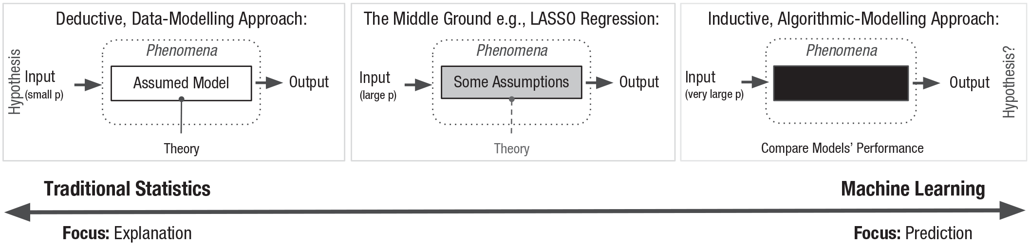
The continuum between a traditional statistical approach and a machine-learning approach. p = set of possible predictors.
We take linear regression as an example, a model that is commonly used in psychology. Linear regression is a traditional statistical technique that aims to predict the outcome variable from predictor variables using additive linear terms. A lot of advanced statistical methods commonly used in psychology, such as structural equation models (SEMs) and mixed-effects models, are an extension of this linear regression. When the number of predictors increases, there is likely an issue of multicollinearity, which makes the parameter estimation and prediction unstable. To stabilize the prediction, linear regression models can be extended to regularized regression models, which include lasso (Tibshirani, 1996), ridge-regression (Hoerl & Kennard, 1970), and elastic-net models (Zou & Hastie, 2005). These models can provide relatively stable predictions with many predictor variables and are often regarded as machine-learning models (Hastie et al., 2009). When the functional relationship becomes more complicated, researchers can alternatively use kernel regression models (Nadaraya, 1964; Watson, 1964), which enable good predictions even when nonlinear relationships exist. However, when doing so, the interpretability of the model suffers compared with the simpler linear model.
We can also think about the other direction. Deep neural-network models are regarded as one of the most powerful classes of machine-learning algorithms across a variety of applications (Shinde & Shah, 2018). But the simplest version of a neural network, called a “perceptron” (McCulloch & Pitts, 1943), can be equivalent to regression with a binary outcome (e.g., logistic regression). Generally speaking, as a model accommodates an increased number of predictors and complex nonlinear relationships, the model naturally becomes more of a black box and is referred to as a machine-learning model. Of course, this is a somewhat simplistic view, and not all statistical tools fit with this continuous perspective. However, the implication of this perspective is that statistical concepts and ideas in one tradition can, to some extent, be transferable to the other tradition. 1 At least by trying to connect the statistical concepts in both fields, rather than learning about them completely separately, we believe psychologists should be able to reach a better understanding of machine-learning methods and vice versa.
Note that when we use the phrase “machine-learning approach” here, we encompass not only the predictive models themselves but also the whole analysis pipeline required to perform machine-learning analyses (for an example of a typical machine-learning pipeline, see Box 2 and Fig. 1). This includes data-preprocessing steps, practices for training and testing models, and a wide variety of different algorithms available to detect patterns in data to use for making predictions. Some of the machine-learning preprocessing procedures can be adapted to the traditional statistical approach or vice versa, for example, certain approaches to missing data. This supports our point that the two approaches are not qualitatively so different, and in the current article, we discuss some critical preprocessing procedures when relevant to our argument (e.g., dimensionality reduction and centering). That being said, in certain machine-learning domains, such as computer vision or natural language processing, data preprocessing is a large and active area of research in its own right (X. Chu et al., 2016). Furthermore, many of the techniques involved in these fields, such as data augmentation (e.g., Shorten & Khoshgoftaar, 2019) or the process of extracting tabular data from unstructured data (e.g., Church, 2017; Mars, 2022; Medhat et al., 2014; Wallach, 2006; Y. Zhang et al., 2010), are not easily comparable with the preprocessing procedure in a traditional statistical approach. Therefore, in the current article, we do not attempt to cover the whole array of literature in this regard.
A Typical Supervised-Machine-Learning Pipeline

Prediction R2, somewhat different to the R2 when fitting a regression model, evaluates how well a model predicts new observations (Scheinost et al., 2019).
For classification problems, the type of metric should be chosen while considering the distribution of data across classes and the cost of an error (Sterner et al., 2023).
In the following sections, we discuss each of the focal challenges that are common in psychological data: (a) a limited sample size, (b) measurement error, (c) nonindependent data, and (d) missing data. In each section, we first introduce how they are approached from a traditional statistical perspective and then suggest possible solutions when using machine learning.
A Limited Sample Size
Approach in traditional statistical methods
Psychological data are often collected directly by researchers to address specific research questions. This has the advantage of allowing researchers to collect precisely the information they need. However, it also tends to be costly and time-consuming. As a result, psychological data sets are usually relatively small, especially in terms of the number of observations (i.e., participants, typically ranging from dozens to hundreds in experiments and hundreds to thousands in surveys). These limited sample sizes make it more challenging to generalize findings from the collected sample to broader populations.
To draw generalized conclusions, psychometrics relies primarily on inferential statistics. Here, researchers assume that the observed sample (i.e., the data they have) is a random sample from the population of interest. Parameters (e.g., means, regression coefficients) estimated from the observed sample are expected to deviate, to some extent, from the true population parameter values. This deviation is referred to as “sampling error.” Although researchers cannot directly observe sampling errors—because the true population values are unknown—under certain distributional assumptions (e.g., multivariate normality), they can evaluate the distribution of sampling errors, known as the “sampling distribution.” In fact, researchers can typically derive the standard deviation of the sampling distribution, known as the standard error, either analytically (i.e., using a statistical formula) or via numerical estimation (i.e., using iterative procedures to approximate solutions). These standard errors are often the basis for determining the statistical significance of parameter values. 2 When distributional assumptions are not met, researchers often use simulation-based approaches to evaluate the sampling distribution (e.g., bootstrapping; see Box 1). Generally, as the sample size (N) increases, sampling error decreases probabilistically (i.e., precision increases; D. R. Cox et al., 2018; Faraway & Augustin, 2018; Riley et al., 2021). In other words, with larger data sets, researchers obtain more information about the population, and the estimated parameter values are less likely to deviate from the true population parameters (i.e., see central-limit theorem, Kwak & Kim, 2017).
Related to inferential statistics, sample-size planning is another important practical step in psychology research because researchers cannot easily collect massive amounts of data. Specifically, researchers can judge whether a certain sample size is sufficient to achieve a high probability of detecting the effects when the effects truly exist. This is called a “statistical power analysis” (Cohen, 1992), and the evaluation of sampling error (e.g., standard errors) also plays a key role here.
How machine learning considers a limited sample size
Ideally, researchers using machine learning will have a large amount of data. But in psychology research, data are still expected to contain a limited number of data instances. When machine-learning methods are used in this setting, there is no obvious quantification of sampling error in most cases (Faraway & Augustin, 2018). For example, when one uses a random-forest model (Breiman, 2001a), one can calculate a metric to assess the predictive performance of the model (e.g., root mean square error) and extract a predictor-importance metric (e.g., permutation importance; Breiman, 2001a); but in most applications, researchers do not see standard errors or p values associated with these quantities (R. Sambasivan et al., 2020). 3 In other words, an explicit metric that reflects uncertainty related to the sample size is typically not seen. With machine-learning methods, then, how can one make a generalized conclusion from a limited sample size?
In a sense, sampling errors are implicitly handled in the machine-learning methodology. This handling occurs through cross-validation and regularization (or feature selection) procedures (see Box 1). By using cross-validation and hyperparameter tuning, researchers aim to find a predictive model that generalizes to new data sets with similar distributional properties. In other words, cross-validation and regularization aim to minimize the effect of idiosyncratic features present in the training data. Therefore, cross-validation and regularization can be regarded as methods for selecting the best machine-learning model while accounting for sampling errors. Note, however, that there are key differences. In machine learning, “generalization” typically refers to the ability of a model to perform well on new data drawn from a similar underlying distribution. “New data” (i.e., the test data) are often a subsample (e.g., 15%–50%) of the full observed sample, future data, or data from a different source. These hold-out samples are eventually known, and how well the model explains the new sample in comparison with the sample it was fit to (i.e., the difference between training error and test error) can be explicitly measured. On the other hand, the traditional statistical approach conceptualizes generalization with regard to the true population, from which the observed data (a tiny sample in comparison) are randomly sampled. This is analogous to randomly sampling data as the training set in machine learning. In both cases, through the random-sampling procedure, the aim is to have distributional similarity—between the sample and the general population in psychology and the training set and test set in machine learning. However, in the traditional statistical approach, the population sample cannot be known because it is too large. In this respect, the machine-learning and the traditional-statistics views conceptualize sampling errors in a slightly different manner. However, both approaches consider how well a model built on a sample generalizes to different data.
To be more concrete, consider a case in which the data contain five possible predictor variables, of which, only one has a true linear relationship with the outcome. In the traditional statistical approach, the four irrelevant predictors are likely to yield nonzero beta values that are not statistically significant. In the machine-learning approach, when an unregularized model is fit to training data, not only the true predictive variable but also many of the other variables will likely show nonzero contributions to the prediction, partly as a result of sampling error. In machine learning, this is referred to as “overfitting” to noise in the data. However, through the model-training and selection process using cross-validation to find the right level of regularization (e.g., L1 norm; Tibshirani, 1996), the contribution of the four nonpredictive features should eventually be eliminated from the final predictive model. The resultant, more parsimonious model is expected to predict the outcome well in new data. This means that after a model has been trained and selected appropriately and the retained features show good predictive performance in the hold-out data, one can say that the model and its features were selected with sampling error taken into account.
Many introductory textbooks in machine learning emphasize generalization to a new sample as a critical feature of machine learning but do not compare this with the concept of “sampling error.” We believe that this situation makes the perceived gap between machine-learning and traditional statistical analysis bigger than the reality. However, as discussed earlier, the concepts of traditional statistics and machine learning are often closely related. As another example, for certain classes of models (e.g., linear regression based), model selection based on cross-validation, specifically, leave-one-out cross-validation (see Box 1), is asymptotically equivalent to the model selection based on Akaike information criteria (AIC; Akaike, 1973, 1974), which is commonly used in traditional statistics to strike a balance between goodness of fit and model complexity. In fact, in cases in which large sample sizes are not available and there are not a large number of models to compare, AIC can be used to select from different machine-learning models on the training data (Midway, 2022). 4 Therefore, both cross-validation and AIC penalize unnecessary complexity with the goal of preventing overfitting. In other words, traditional statistical approaches also implicitly incorporate a model-selection procedure similar to cross-validation.
Acknowledging the link between a traditional-statistics approach and machine-learning approach, we can also think of ways to leverage the knowledge of one approach to enrich the other. One such example is the quantification of sampling error for predictor-importance estimates from machine-learning models. In traditional statistics, it is not only considered whether a parameter is meaningful after taking into account sampling error (i.e., statistical significance) but also how accurate these parameter estimates are likely to be (e.g., by using confidence intervals). Imagine researchers who have a machine-learning model that shows good performance in hold-out test data. The model may also include some interpretable values to represent predictor importance (e.g., Gini impurity for a random forest; Breiman, 2001a). However, if the training and/or test data are small, the model-performance and predictor-importance values are likely to be inaccurate because of sampling error. In machine learning, sampling error is typically reflected only in poor model performance and not in the explicit quantification or estimation of sampling error related to the predictors’ importance. Thus, by simply analyzing the predictor-importance estimates, particularly if they are calculated on the training data (for further discussion on what data should be used, see Lavelle-Hill et al., 2025), the researchers do not know how generalizable their variable importance findings are to other samples.
Although it is not common practice in the machine-learning community to routinely quantify sampling error explicitly (Faraway & Augustin, 2018), the computation of uncertainty related to machine-learning performance estimates has nonetheless been an active field of research (for a review, see Nemani et al., 2023). One useful method is bootstrapping (see Box 1). This method refits the selected model to predict the outcome on multiple generated (e.g., bootstrapped) data sets from the same distribution, providing researchers with an indicator of sampling error (e.g., see Bouthillier et al., 2021; Lavelle-Hill et al., 2021; Michelucci & Venturini, 2021; Nadeau & Bengio, 2003). Bootstrapping is a flexible and powerful method that is used in both traditional statistical analysis and machine learning because it does not require distributional assumptions (Efron & Tibshirani, 1994). In machine learning, it has been used to quantify the sampling error associated with the overall prediction performance (Bouthillier et al., 2021; Dietterich, 1998; McPherron et al., 2022; Michelucci & Venturini, 2021). However, in principle, it can also be used to quantify the effect of sampling error on estimates of predictor importance, given a model.
Sample-size planning/evaluation, which is highly related to generalizability in the traditional-statistics approach, has attracted even less attention in the field of machine learning. Unlike traditional statistics, the adequacy of the sample size in machine learning is usually only implicitly evaluated in relation to the model performance and has not been seriously considered beyond this (e.g., Dhiman et al., 2023). Some fields (e.g., psychiatry) have developed their own heuristics, such as “number of predictors * 10” rule (Concato et al., 1995; Peduzzi et al., 1995, 1996). However, recent research has demonstrated that many human data sets used to build and evaluate prediction models have been undersized, increasing the risk of (upward) bias (Vabalas et al., 2019; Wynants et al., 2020) and potentially giving rise to inaccurate conclusions (Dhiman et al., 2023). Several studies have provided formulas to evaluate the adequacy of sample size in certain applied-machine-learning fields (e.g., in medicine; Riley et al., 2019a, 2019b, 2020; van Smeden et al., 2019), but the extent to which these methods can be extended to different classes of machine-learning models and other types of data, such as psychological data, is still unclear.
Measurement Error
Approach in traditional statistical methods
In the natural sciences, researchers are typically dealing with quantities such as chemical compounds or physical matter, which can be measured directly. In contrast, in psychology, researchers often want to measure intangible phenomena, such as attitudes, beliefs, emotions, states, and traits. To assess these ambiguous concepts, it is unavoidable that measures are accompanied by some amount of measurement error—the deviation of the measured values from the true value of the concept (given the sample; McDonald, 2013). Measurement errors reflect various factors irrelevant to the concept itself they want to measure. They exist because the “true” constructs can be measured only indirectly, for example, by asking questions about phenomena that theoretically reflect the construct. The problem is that almost all standard statistical models—especially regression models and their extensions—assume that variables are perfectly measured. However, when measurement errors are present, parameter estimates become biased (Bound et al., 2001).
One may have the intuition that measurement error simply attenuates the results, and thus, researchers should simply keep this in mind when interpreting the effect size and p values. This is wrong. When there are multiple predictors in a regression model, for example, measurement error can wrongly strengthen a positive association or even reverse the effect (Bound et al., 2001; Brunner & Austin, 2009; Cohen et al., 2013). The direction of the bias is almost completely unpredictable when there are several correlated predictors. Even if a variable is perfectly measured, if another variable in the model is measured with error, the regression coefficient for the perfectly measured variable can be biased. 5 Because of the bias, Type 1 error rates also naturally inflate—even if the variable has no effect (and regardless of whether the predictor itself was perfectly measured), the variable may show a significant effect if other predictors in the model suffer from measurement error (Brunner & Austin, 2009; Cole & Preacher, 2014). Increasing the sample size cannot counter the bias (van Smeden et al., 2020). In fact, when the bias is present, larger sample size actually increases Type 1 error rates.
Although some sophisticated models have been proposed for variables with measurement errors (especially in econometrics; e.g., Fuller, 2009), the issue is hard to resolve because the measurement error needs to be quantified in the first place. One straightforward strategy commonly used in psychology is to assess constructs (e.g., personality traits) using multiple items. If there are inconsistent responses to the multiple items assessing the same construct, then they should be deemed as measurement error. With multiple items per construct, latent variable modeling can then be applied, for example, through the commonly used SEM framework (Bollen, 1989). The SEM framework is a combination of factor analysis (FA; Fruchter, 1954; P. Kline, 2014) and path models to estimate the commonality of individual items by supposing a latent factor (an unobserved variable that is inferred from observable variables) that researchers can flexibly include in a regression model. The fundamental assumption is the existence of a hidden “true score” behind the measurement, which reflects a psychological construct of interest, and researchers are concerned with the relationship between this true score and the outcome.
How machine learning can address measurement error
In the machine-learning community, it is well known that the quality of the data plays a large role in the predictive capabilities of models, and thus, much attention needs to be paid to data cleaning and augmentation (X. Chu et al., 2016; N. Sambasivan et al., 2021; Shorten & Khoshgoftaar, 2019). For example, Polyzotis et al. (2019) described data validation as “on par with the algorithm and infrastructure used for learning.” Despite this, and aside from the potential impact on prediction performance, there has been limited discussion on the effect of measurement error on the machine-learning model and its interpretation (for exceptions, see Datta & Zou, 2020; Jacobs & Wallach, 2021; Jacobucci & Grimm, 2020; McNamara et al., 2022). This may be because strong assumptions on the validity of data are not needed for prediction in machine learning. However, the difference between an unobservable construct and its measurement can lead to misinterpretation and biased algorithms (e.g., Jacobs & Wallach, 2021). Furthermore, measurement error, more generally, is not unique to psychological data. Many of the data sets used to train machine-learning algorithms will also contain measurement error (McNamara et al., 2022; Morgenstern et al., 2021). But is this error taken into account in machine-learning models, and does it need to be?
On the one hand, certain machine-learning approaches are arguably highly successful at reducing measurement error because they have the capability to learn underlying representations of the feature space. This can be done using unsupervised methods and is an alternative to manually engineering features (e.g., by taking the mean or median of the multiple measurements). The process typically occurs within a (optional) step of the supervised-machine-learning pipeline known as “dimensionality reduction” (Ghojogh et al., 2023) before the model is fit (Bartal et al., 2019). 6 Dimensionality reduction in machine learning is the process by which the number of input features is reduced, either by feature-selection or feature-compression methods (the combining of many features into a smaller number of model inputs). In machine learning, this is typically performed with the goal of avoiding the curse of dimensionality (Bellman, 1957; see Box 1), thus aiding prediction performance and easing computational costs.
When the feature space is compressed, higher-order dimensional features (or “components”) are arguably more reliable and thus suffer less from measurement error. This is because the selected components are capturing the dimensions in the data with the highest variance, making them less sensitive to noise (Greenacre et al., 2022). Furthermore, simplifying the representation of the data (reducing the dimensions) means there are fewer opportunities for measurement error to occur (Hellton & Thoresen, 2014). In addition to principal-components analysis (PCA), which is also commonly used in psychology (Bryant & Yarnold, 1995), methods used in machine learning include nonnegative matrix factorization (NMF; D. Lee & Seung, 2000; Y.-X. Wang & Zhang, 2012) and independent-component analysis (ICA; T.-W. Lee & Lee, 1998). 7 Similar to FA (Fruchter, 1954; P. Kline, 2014) and PCA, these methods produce components that the original variables load onto. Although (confirmatory) FA and PCA are similar (Hinton et al., 1994; Roweis & Ghahramani, 1999) and capture variance or covariance structures (for further discussion on the similarities and differences, see Widaman, 2007), ICA aims to maximize the statistical independence between the extracted components (T.-W. Lee & Lee, 1998). NMF uses matrix factorization to compress (nonnegative) data with additive properties (e.g., images; Aonishi et al., 2022; Guillamet et al., 2003) into two matrices (plus some error)—the H matrix, containing the loading of features onto components, and the W matrix, containing the loadings of data instances onto components. In addition, a number of nonlinear methods have been proposed, for example, kernel PCA (Schölkopf et al., 1998). For an overview of nonlinear methods, see Van Der Maaten et al. (2009), and for visualization methods, see Rudin et al. (2022). For unstructured text data, there are also natural-language-processing methods to extract higher-order topics or linguistic features (e.g., topic modeling; Blei & Lafferty, 2009; Kao & Poteet, 2007).
In a supervised-machine-learning pipeline, the feature-compression process often occurs without being guided by theoretical concepts. Instead, the goal is to find a lower-dimensional data representation while retaining as much of the original information as possible (Montano, 2014). This is in contrast to SEMs/FA, which usually works on theoretical or conceptual grounds (although, see also exploratory SEMs; Marsh et al., 2014). Although unsupervised-machine-learning methods can reduce measurement error to some extent (i.e., increase measurement reliability; Greenacre et al., 2022), their effect remains somewhat limited. It is also possible that all variables are measured poorly and that the compressed components pick up on the systematic (i.e., correlated) measurement error. Furthermore, it is known from the psychometrics literature that such point estimates of aggregated features—regardless of the method used—are still contaminated by measurement error because they do not account for randomness (Lechner et al., 2021). In addition, particularly when driven by data rather than theory, the resultant components are not guaranteed to be interpretable (Rudin et al., 2022). Thus, as input features get merged, this can reduce model interpretability and make it more difficult to understand the contribution of individual features.
Aside from the reduction of measurement error that may occur as a (typically unintended) consequence of feature-compression approaches, there is relative inattention to measurement error in machine learning and its effects in the model-fitting phase (i.e., its impact on coefficients in a regression-based machine-learning model). This is because machine learning, at the extreme end of the continuum, is primarily aimed at maximizing the prediction accuracy given the features (i.e., measurements) available (Breiman, 2001b; Hofman et al., 2021; Mullainathan & Spiess, 2017; R. Sambasivan et al., 2020). Given this goal, it may not make sense to consider or discuss the predictive accuracy of a feature before being disturbed by measurement error (the true scores) or how the predictive accuracy of the true scores might be biased. Taking this perspective, measurement errors are typically of concern only if they attenuate the overall prediction accuracy and, hence, if this information can be used to change data collection or the modeling process in a way that would improve predictive performance. In other words, when there is a true relationship, it is better to have features with high reliability not because such features more closely reflect true scores but because they generally predict the outcome better. In addition, from a purely prediction standpoint, arguably, if the measurement error of a feature turns out to increase prediction accuracy (because the error happens to be correlated with the outcome), one should retain such a “contaminated” feature (as viewed from a traditional-statistics perspective) in the predictive model.
That said, we believe that there is a clear benefit of thinking more explicitly and seriously about measurement error in machine learning. First, by explicitly accounting for measurement error in machine-learning models, researchers may be able to achieve a better prediction. This is one potential consequence of dimensionality reduction (Bellman, 1957). Yet a more explicit method of dealing with measurement error could yield even bigger predictive gains. More broadly, by assuming measurement errors, researchers implicitly impose theoretical constraints on features. A substantial body of literature suggests that (valid) theoretical constraints can enhance machine-learning performance (e.g., Karniadakis et al., 2021; Schölkopf et al., 2021; Singh et al., 2019). Second, when importance of individual features are interpreted, measurement error could lead to misleading results (see also Jacobucci & Grimm, 2020; Luijken et al., 2019; McNamara et al., 2022). At least in the case of regression-based models, as noted above, measurement error could change the regression weight even in the opposite direction. In more complex models, such as random forests or XGBoost, it is possible that there is a positive bias toward selecting features with lower measurement error, similar to biases in favor of features with higher cardinality (Kononenko, 1995; A. P. White & Liu, 1994). Yet there has been little research that has explicitly examined the impact of measurement error on predictor importance and selection in machine-learning models.
One potentially fruitful avenue may be to combine machine-learning algorithms with the SEM framework, for example, using regularized SEM (Brandmaier & Jacobucci, 2023; Jacobucci et al., 2016, 2019; X. Li & Jacobucci, 2022) or SEM tree/forest algorithms (Brandmaier et al., 2013, 2016). With these models, theoretical latent variables can be used as features to predict the outcome combined with regularization mechanisms and complex nonlinear functions. At the same time, SEMs typically define measurement error in a very specific way (although there are some exceptions), that is, the unique variance that is not commonly shared by the items (the shared part forms a latent variable; Bollen & Lennox, 1991). In other words, some important item-specific elements might also be regarded as measurement error and discarded from the analysis (Donnellan et al., 2023). This is despite recent research showing that a model including item-specific effects could have higher predictive power than a model with only scale scores (McClure et al., 2021). Therefore, although there is promise in these recent methodological developments, they address only one specific definition of measurement error commonly found in psychological data.
Nonindependent Data
Approach in traditional statistical methods
Most of the traditional statistical analysis methods in psychology assume data independence, in which each data point is treated as independent of the others. However, psychological data often exhibit a hierarchically nested structure. For instance, data points can be nested within individuals or students within schools. In such cases, the data points are no longer independent from one another because data points within the same upper unit (e.g., person, school) are likely to be more similar than data points from different upper units. The degree of dependency between groups can be quantified using measures such as intraclass correlation (ICC; Bartko, 1966).
If one analyzes nonindependent data with standard statistical methods, generally, two issues emerge, and the extent of the problem becomes greater as ICC increases. First, the analysis could bias causal estimates because the upper unit (e.g., person, school) could be regarded as a confounder, directly influencing the variables of interest (Rohrer & Murayama, 2023). Second, the analysis would tend to underestimate the sampling error because the analysis assumes that all the cases have unique and independent information despite the data actually including redundant, shared information. To address these issues, researchers have proposed various statistical methods, such as mixed-effects modeling (or hierarchical linear modeling; Gałecki et al., 2013), robust standard errors (Hoechle, 2007), and generalized estimating equation (Zeger et al., 1988). These methods appropriately take into account the variance attributed to the upper units, allowing researchers to make appropriate statistical inferences. These methods can also address the issue of confounds by simple extensions, such as using a cluster-mean-centering approach (Enders & Tofighi, 2007) or latent variable modeling (Silva et al., 2019). They eliminate the between-clusters differences from the data manually (i.e., cluster-mean centering) or statistically (i.e., latent variable modeling); thus, the features associated with the clusters can no longer be confounders. Moreover, mixed-effects modeling, which is widely used in psychology, takes advantage of hierarchical data structures to flexibly answer various research questions (Raudenbush & Bryk, 2002). For example, if regression slopes are different between clusters (random slopes), researchers can include predictors at the cluster level to explain these cluster differences (i.e., cross-level interactions).
How machine learning can address nonindependent data
In practical applications of machine learning at the extreme end of the continuum, one could argue that the data structure is not crucial in the context of machine learning’s primary goal, to find an optimal predictive function (Breiman, 2001b). From this purist perspective, one may believe that the data’s underlying structure need not be a concern as long as the predictions are accurate. However, when viewed through the lens of traditional statistics, it can be pointed out that the search for an optimal prediction is undermined by ignoring the nonindependence of data. More specifically, neglecting the presence of nonindependence leads to the underestimation of sampling error, ultimately resulting in overfitting, as we illustrate below (for simulation work, see also Hu et al., 2023,).
Consider an example in which a researcher has data from 10 groups, each comprising 100,000 individuals in the training data set. The individuals within each group are highly similar, although those between groups are significantly different. The ICC would be high in such a scenario. If these group distinctions are disregarded and a standard cross-validation methodology (e.g., K-fold) is employed without considering nonindependence, the model is likely to exhibit overfitting. This occurs because the modeling and cross-validation procedures assume that the 10 × 100,000 data points are independent. Consequently, the model might incorrectly identify certain group-specific features as important predictors even if these features are noncausal and correlate with the outcome by chance (Hornung et al., 2023; Roberts et al., 2017). In other words, the model would be falsely confident (exaggerated by the large sample sizes; Reid, 2018) that the effects of these features were not the result of sampling error.
Although there is not yet a “gold standard” for how to deal with nested data structures, there are two general strategies employed in the current supervised-machine-learning literature to address the underestimation of sampling errors. 8 First is a simple, practical solution, which we call the “cluster-as-features” approach: Researchers include the upper units as predictors (e.g., a categorical class variable for tree-based approaches or a set of dummy variables for classes in a regularized regression; see also Kilian et al., 2023). This method is analogous to a fixed-effects model in the traditional-statistics literature (Gardiner et al., 2009; McNeish & Kelley, 2019; Sommet & Lipps, 2024), which is known to address the underestimation of standard error. This clusters-as-features approach could also help to improve predictions. For example, if there are big differences between schools in academic achievement, information about which school a student attends has good predictive utility for the student’s achievement score. Using this method, potential interactions between the upper units and lower units (i.e., subgroup effects) could also be modeled. However, one fundamental limitation of the clusters-as-features approach is that it cannot easily make a prediction about a new cluster (below, we discuss the implication in relation to inflated performance estimates)—this is also the limitation of fixed-effects models in traditional statistical approaches. If there are 50 schools in the data, the clusters-as-features approach could make a good prediction for only those 50 schools, and the model cannot predict a new class because there is no such (dummy) variable representing the new class in the model. Note that by integrating certain unsupervised approaches, such as similarity-based methods (Ding et al., 2014) or neural-network approaches that learn continuous embeddings (e.g., Mars, 2022), one could get around this problem. However, in a typical supervised pipeline, the utility of such a predictive model would be limited in this context.
The second is a more technical solution. Researchers have developed new machine-learning methodologies that statistically deal with the nonindependence of data. These methods are useful in situations in which data collection might be biased by the data clusters (e.g., the data were collected from different labs) and one wants to control for this effect rather than use it as a predictor. The focus has been on combining mixed-effects models with different machine-learning models to account for the nonindependence, for example, combining linear mixed-effects models with lasso regression (Groll & Tutz, 2014; Pan & Huang, 2014; Schelldorfer et al., 2011), decision trees (Fokkema et al., 2018; Fu & Simonoff, 2015; Hajjem et al., 2011; Kundu & Harezlak, 2019; Ngufor et al., 2019; Sela & Simonoff, 2012), random forests (Calhoun et al., 2021; Capitaine et al., 2021; Hajjem et al., 2014), gradient tree boosting (Salditt et al., 2023; Sigrist, 2022), and neural networks (Mandel et al., 2023; J. Wang, 2025; Xiong et al., 2019). Promising recent work has also focused on developing generalized model-agnostic frameworks (Kilian et al., 2023). The general idea here is that the fixed-effects and random-effects parts are separately estimated via alternate iteration: The fixed-effects part of the model is estimated by a standard machine-learning model, and the random effects are estimated by a standard method in mixed-effects modeling (e.g., restricted-maximum-likelihood method).
In many cases, incorporating the random effects has improved predictive performance beyond linear mixed-effects models and the original machine-learning algorithm (e.g., Hu et al., 2023; Ngufor et al., 2019; Sela & Simonoff, 2012). However, these hybrid models are not yet commonplace in the applied-machine-learning field, and the availability of the software, for example, in Python (the programming language used most commonly for machine learning; Hao & Ho, 2019; Raschka, 2015), is still somewhat limited. For example, Scikit-learn (Pedregosa et al., 2011a), the most popular Python package for machine learning (Hao & Ho, 2019), does not include such models. 9 Hierarchical Bayesian models can also be used to capture dependencies between different levels, offering robust estimates (Bharadiya, 2023). However, both Bayesian machine-learning and mixed-effect machine-learning methods present challenges in terms of computational complexity and scalability when dealing with data sets with a large number of predictors (Bharadiya, 2023; Kilian et al., 2023).
The issue of confounding from the cluster level can be addressed in the same way as the traditional statistical approach. Specifically, researchers could cluster-mean center the features (both the outcome and independent variables) before applying machine-learning methods (e.g., as in Deininger et al., 2023). 10 In psychology, this variable transformation is applied to examine “within-clusters” effects, which are less confounded by the cluster-level effects (Hamaker & Muthén, 2020). However, from the perspective of pure prediction, such centering approaches do not make as much sense because they would typically decrease the prediction performance by potentially throwing away important predictive information (i.e., cluster-level effects) from features. However, the cluster-mean-centering method can provide a clearer interpretation of the effects by eliminating potential confounds. The decision to do cluster-mean centering will depend on the purpose of the analysis—whether one prioritizes prediction or interpretation. Researchers should be aware that the decision fundamentally changes the way the results can be interpreted.
In situations in which the ICC is high, it can be advantageous to leverage the clustered structure of the data to enhance predictive accuracy. One effective approach is to create additional model features derived from each cluster, such as the mean, median, mode, standard deviation, or entropy of relevant predictor variables within that cluster. By incorporating these cluster-level statistics as predictors in the model, researchers can use the shared variance within clusters, ultimately improving the performance of predictive models. In psychology, several studies have shown that cluster-level predictors have substantial contributions to various outcomes beyond the original predictors—often called “contextual analysis” (Firebaugh, 1978) or “compositional models” (Harker & Tymms, 2004). However, by including additional features in the model, researchers are increasing the dimensionality, which can lead to both unstable predictions (Bellman, 1957) and longer run times. Researchers will likely need to be guided by theory or require additional feature-selection methods to decide which variables to aggregate at the cluster level and include in the model.
In machine learning, analysts must consider data nonindependence when choosing a model-evaluation method and reporting on performance in relation to the research question. For example, when applying cross-validation, researchers can split the data into training and test/validation data either between clusters (between-clusters split) or within clusters (within-clusters split; Roberts et al., 2017). If the ICC is high, the within-clusters split should show a higher predictive performance in the test/validation data because both training and test data include examples from the same clusters. For a between-cluster splits, also referred to as “block” (Roberts et al., 2017) or “grouped” 11 cross-validation, the test set contains data in clusters that have not been seen by the model in training. If a researcher is interested in the prediction for only those clusters the model has seen examples of, a within-clusters split makes sense (and a clusters-as-features approach would be useful). However, if one wanted to estimate the performance of a model predicting a new cluster, a between-clusters split would give researchers more accurate, realistic estimates (Hornung et al., 2023). The choice should be clearly articulated and justified so that any information leaked from the test set to the train set (see “data/information leakage” in Box 1) caused by the ICC being high (i.e., similar data occurring in both train and test sets) does not give misleading, overly optimistic performance estimates (Farokhi & Kaafar, 2020; Gibney, 2022; Guignard et al., 2024). This example highlights that data nonindependence creates a multitude of epistemic questions that researchers should consider before making analytic decisions.
Missing Data
Approach in traditional statistical methods
Missing data is common in psychological research. For example, in surveys, missingness can occur because of dropout, technical errors, or the skipping of responses because of inattention, confusion, boredom, or study design (e.g., Graham et al., 2006). In longitudinal data, dropout typically occurs over time. Sometimes, researchers might be tempted to simply throw away these missing data before the analysis (called “complete-case analysis”). However, this brings about two issues. First, complete-data analysis eliminates all partially informative data (i.e., cases that have missingness for only a few but not all the variables), potentially influencing the precision (e.g., standard error) of parameter estimates. Second, when the missingness does not occur completely at random, systematic bias may be introduced into the results (Enders, 2022, 2025).
The traditional statistical literature has offered a number of techniques to handle missing data (for a comprehensive overview, see Enders, 2025), most notably multiple imputations (Little & Rubin, 2019; Rubin, 1987, 1996; Schafer, 1997; Van Buuren, 2018) and (full information) maximum likelihood (Arbuckle et al., 1996; Baraldi & Enders, 2010; Beale & Little, 1975; Dempster et al., 1977). 12 Full information maximum likelihood is a method in which missing values are not replaced or imputed but are instead handled directly when calculating the likelihood function. This method is especially popular in SEMs (R. B. Kline, 2012). Multiple-imputation methods impute missing data from a model that a researcher specifies (e.g., multiple regression). Unlike single-imputation methods, these methods incorporate the uncertainty of the imputed values by generating multiple different imputed data sets (typically five to 20, depending on the proportion of missingness; I. R. White et al., 2011) using (model-based) random errors. The analysis is then carried out in each of the imputed data sets, and the results are either aggregated or adjusted to account for the uncertainty (e.g., using Rubin’s rules; Rubin, 2018).
One critical but often overlooked assumption of multiple imputation is that researchers correctly specify a model for missing data (Van Buuren, 2018). For example, if a researcher believes that a missing value is best predicted by interaction effects of other variables, these interaction terms should be included in the model predicting missing values (Enders, 2025). When assumptions are met, full-information-maximum-likelihood and multiple-imputation approaches will typically produce similar results (Collins et al., 2001). Both methods allow researchers to make full use of the data and, more notably, can provide unbiased parameter estimates with correct standard errors even when missingness is not completely at random. Specifically, if the missingness of a variable is systematic and the systematic missingness can be explained by the other variables in the model (this condition is called “missing at random” [MAR] 13 ), the methods produce unbiased parameter estimates and correct standard errors (Enders, 2025). Of course, one cannot know whether the MAR assumption is met in practice, but in general, these methods are more robust to systematic missingness than the complete-case analysis (Sterne et al., 2009).
How machine learning can address missing data
In machine learning, maximum-likelihood-based approaches are available for some models (e.g., Ghahramani & Jordan, 1993; Williams et al., 2005); however, many models (e.g., tree-based algorithms) do not use a likelihood function to estimate parameters. Instead, several machine-learning models can handle missing data as inputs or treat missingness as a meaningful feature (You et al., 2020). For example, many tree-based models have in-built methods to deal with missing data (Breiman et al., 1984; T. Chen & Guestrin, 2016; Friedman, 2001) by incorporating missingness as a feature in the model (i.e., by allowing missingness to be a criterion to split on), making available only the nonmissing information for each split decision and distributing the missing data across the daughter nodes in accordance to the distribution of the nonmissing values (i.e., the C4.5 algorithm; Quinlan, 2014), or using surrogate splitters that emulate the primary splitter (the best split decision), which are called on when the primary splitter is missing (Breiman et al., 1984; Umezawa et al., 1995). For further strategies, see Gavankar and Sawarkar (2015) and Twala (2009). Likewise, the XGBoost algorithm, an ensemble decision-tree method that builds trees sequentially, can also handle missing data. At each split point, it assigns a default branch for the missing data to follow. The default is the branch that minimizes the loss function (quantification of the difference between the predicted and the actual values) the most when the missing data follow it (T. Chen & Guestrin, 2016). In other words, it attempts to handle the missing data in a manner that improves prediction. In certain applications, such as predicting mental-health outcomes, leveraging the extent and presence of missingness has been shown to bolster predictive performance (Wu et al., 2022), and many machine-learning methods can capitalize on this.
Extensions to other machine-learning models have also been proposed to enable the handling of missing data, for example, for random forests (Xia et al., 2017), SVMs (Chechik et al., 2008; Pelckmans et al., 2005), and deep-learning models (Bengio & Gingras, 1995; Goodfellow et al., 2013; Śmieja et al., 2018). Using algorithms that can take missing data as inputs allows the data to be modeled in relation to the missing-data context rather than trying to emulate a context in which no data are missing. This prevents impossible scenarios from occurring in the imputed data, such as pregnant fathers (Van Buuren et al., 2006). It can also produce significant computational savings (Chechik et al., 2008). However, it has been shown that some of these algorithms that handle missing data are inferior to first imputing the data and then fitting a model (e.g., Feelders, 1999). Furthermore, selecting a certain machine-learning model a priori because it handles missing data or using this as a criterion to restrict the model search space may undermine the model-selection process by causing a suboptimal model to be chosen. How a particular model handles missing data may also introduce unknown bias (You et al., 2020). Thus, many researchers prefer to keep the handling of missing data as a preprocessing step, separate from the model-selection process (Nijman et al., 2022).
In line with this idea, a flexible and commonly used strategy in machine learning is single imputation (Nijman et al., 2022; You et al., 2020). Single imputation involves creating a single imputed data set 14 (without adding random error) and using the imputed data to make predictions. In their review, Nijman et al. (2022) found that 61% of machine-learning analyses that imputed data used this approach. However, it can take various forms (Thomas et al., 2020). The most naive strategy is to simply fill in the missing values with a constant, such as the mean, median, mode, or most common category—often referred to as “simple imputation” (Pedregosa et al., 2011c). A more rigorous method, multivariate imputation (e.g., Pedregosa et al., 2011b; Van Buuren & Groothuis-Oudshoorn, 2011), uses a statistical model or supervised-machine-learning algorithm to predict the missing data points (as outputs) given the existing values (inputs). A common implementation is to iterate over the columns in a round-robin fashion, predicting the missing values in the target column using the other features in the data (e.g., Pedregosa et al., 2011b). In addition to regression (Z. Zhang, 2016b), different machine-learning algorithms have been proposed for multivariate imputation, many of which have been shown to yield more accurate predictions than statistical methods (e.g., Jerez et al., 2010). Commonly used methods include K-nearest neighbors (Z. Zhang, 2016a), Bayesian ridge regression (Tipping, 2001), and random forests (Breiman, 2001a). In addition, state-of-the-art methods continue to be developed, including the use of generative adversarial networks (Luo et al., 2018; Yoon et al., 2018), graph neural networks (You et al., 2020), autoencoders (Gondara & Wang, 2018; Vincent et al., 2008), and different deep-learning methods (e.g., Chai et al., 2020). Such methods can additionally be used for data augmentation and the generation of new synthetic data (e.g., Y. Chen et al., 2020). The attractiveness of single imputation is that once the imputed data are created, any type of machine-learning method can be applied as usual. However, single-imputation methods can be biased by the model selected and the specific initialization of the default values (You et al., 2020). Thus, machine-learning researchers may try out different imputation methods in the training phase to find the one that maximizes prediction accuracy in the validation data. In this way, imputation can be viewed as a hyperparameter and part of the pipeline that is optimized for prediction.
When using single imputation, machine-learning researchers commonly apply the following two constraints. First, it is common practice to impute missing data based solely on the training data (but see also Gunn et al., 2023). This simulates the real-world scenario in which the test data are unknown during training and all instances in the test data may not have been seen when predicting a given instance. If information from the test data is used in the training phase to impute the missingness, it contaminates the training data by making it artificially more similar to the hold-out test set. This is another example of data/information leakage (see Box 1) and can lead to the potential overestimation of the prediction performance in test data (Gibney, 2022). Second, given the goal of finding the best predictive function that generalizes to out-of-sample data, researchers in machine learning typically do not impute the outcome variable (Jerez et al., 2010). This is because supervised-machine-learning methods are evaluated by comparing the model’s predictions with “ground truth” labels (the actual values). Therefore, the evaluation of the model’s performance would be compromised if the model’s prediction were evaluated against the predicted value from an imputation function with unknown fidelity to the true value. Furthermore, imputing the outcome variable is generally avoided in machine-learning workflows because it replicates the modeling effort carried out in the primary analysis. During the imputation phase, researchers fit a predictive model that uses the available features to estimate the missing outcome values. Immediately thereafter, the main analysis fits yet another model—based on the same set of features—to predict the outcome. Both steps pursue the same objective of learning the optimal mapping from predictors to outcome, so the imputation stage contributes no additional information while duplicating computational work. Consequently, outcome-variable imputation is seldom employed in contemporary machine-learning practice.
Given the goal of prediction, single-imputation methods make sense because they attempt to impute data in a way that would preserve the existing predictive relationships without throwing away missing data. From the perspective of traditional statistical analysis, however, we raise a point for discussion—whether imputation methods in machine learning need to take into account the uncertainty because of missingness. As an (extreme) example, imagine a predictor variable has 90% missing data and the rest of the data (10%) showed some observed correlation with the outcome. It is reasonable not to take this observed correlation at face value (i.e., generalize it to the full data set) because the amount of data is comparatively small. Multiple imputation naturally accommodates this intuition by taking into account the uncertainty associated with the amount of missing data. Single imputation, however, does not because data with single imputation do not contain any information distinguishing the imputed values (which include uncertainty) from the real observed values. Consequently, the prediction model selected on the imputed training data may overfit to the imputation function because the model considers the imputed data as equally valid as the observed data—potentially resulting in suboptimal performance in the test data. Furthermore, how would one interpret a model that found the feature with 90% imputed data highly predictive?
In practice, when one has a very large number of possible predictors, it is usually deemed reasonable to discard features with high missingness (Nijman et al., 2022), like the one in the above example, because of the high amount of uncertainty (unless there are theoretical or causal reasons to retain it; Batista & Monard, 2003). This can be considered part of a feature-selection process (García et al., 2016). Following this intuition, researchers might use some rule-of-thumb (e.g., > 50% missing 15 ) to decide whether to drop or impute a predictor variable (Lin & Tsai, 2020). Such a threshold will depend on domain knowledge, the proposed/selected model, and the number of features and instances in the data (i.e., whether it is important to preserve features; Batista & Monard, 2003). However, there are no well-established rules, and it is usually left to the researcher’s discretion (Emmanuel et al., 2021).
Because single-imputation methods do not account for uncertainty because of missingness, should multiple-imputation methods be used instead for machine-learning analyses? This sounds like a reasonable suggestion, but in practice, it is more complicated (Khan & Hoque, 2020). Aside from the obvious computational challenge because of handling multiple data sets, the problem is that there is no established method like Rubin’s rules (Rubin, 2018) to integrate the results from multiple data sets (in both the training data and test data). For example, training a model on different imputed data sets will likely result in different hyperparameters and features being selected in each data set (Molnar et al., 2020), and it is not clear whether it makes sense to integrate results from models with different hyperparameters/predictors. There are other procedural considerations for which different researchers have different proposals (e.g., whether imputed data should be analyzed separately or stacked together and analyzed as a single data set; Gunn et al., 2023), but there has been little consensus on which procedure to use. Practical applications of multiple imputations in machine learning seem to focus mostly on averaging the results and less on the variance across different imputations (e.g., Khan & Hoque, 2020; but see Alasalmi et al., 2015). This means that the uncertainty of the imputed data is typically not taken into account by the model (Emmanuel et al., 2021; Graham, 2009), which could result in misleading interpretations being made.
General Discussion
In this article, we have taken the reader through some of the challenges of using a machine-learning approach that are inherent in the typical characteristics of psychological data. Specifically, these involve handling a limited sample size, measurement error, nonindependent data, and missing data. Several prominent articles have discussed the application of a machine-learning approach in psychology (Adjerid & Kelley, 2018; Bzdok, 2017; Dwyer et al., 2018; Elhai & Montag, 2020; Hofman et al., 2017; Hullman et al., 2022; Orrù et al., 2020; Rocca & Yarkoni, 2021; Tay et al., 2022; Van Lissa, 2022; Yarkoni & Westfall, 2017). For example, Liem et al., 2018 outlined different options for integrating machine learning into analysis pipelines in psychology, including the direct substitution of a traditional statistical model for a machine-learning model. However, such integration is typically not straightforward. Switching to a machine-learning model can affect decisions along the whole analysis pipeline, including the data preprocessing (Shmueli, 2010). In general, we found there to be a lack of work that directly addresses the compatibility of machine learning with characteristics that are typical of psychological data. In Table 1, we provide an overview of the potential solutions we have discussed and their remaining limitations. In this section, we reflect on our discussion of each challenge, followed by a broader discussion of future research possibilities.
A Summary of the Four Challenges Discussed That Emerge When Using Machine Learning to Analyze Psychological Data

Note: SEM = structural equation modeling; ML = machine learning; PCA = principal-components analysis; NMF = nonnegative matrix factorization; ICA = independent-component analysis; MI = multiple imputation.
In the traditional statistical approach, given the limited sample size in typical psychological data, the evaluation of sampling errors plays a central role in data analysis. On the other hand, although the machine-learning approach implicitly takes into account sampling errors to some extent in the cross-validation procedure, the explicit quantification of sampling errors is still rare. This is problematic—when researchers see a standardized prediction R2 of .3 in the test data, for example, the interpretation should be different depending on whether the results are based on a large or small sample size. Without the explicit quantification of sampling errors or a standardized evaluation of sample-size adequacy, objective interpretation of the results is difficult. We recommended bootstrapping as a flexible method for estimating the sampling distribution of a model performance metric or variable importance value. Bootstrapping can also enable the use of statistical tests (e.g., to see if the model performs significantly better than a baseline model; Dietterich, 1998) without needing to meet parametric assumptions.
At the same time, more effort is needed to establish concrete guidelines to use such procedures to quantify the sampling errors. For example, when using bootstrapping to assess the uncertainty of either the model’s predictions or the predictor-importance values, the question arises as to how the model’s hyperparameters are estimated before refitting it to each new sample. One possibility is to fix the hyperparameters before refitting (Michelucci & Venturini, 2021). This is a practical option, mostly because of computational reasons but also because of the high likelihood of the model and the explanation it produces varying drastically across samples if hyperparameters are allowed to vary (e.g., see Molnar et al., 2020). For example, decision trees have been shown to change a lot in relation to very small changes to the input data (Breiman, 2001a). Thus, if the goal is to understand the uncertainty of a particular model’s prediction, as opposed to the underlying data, it makes most sense to fix the model’s hyperparameters. However, there has been little research that has empirically examined the consequences of such decisions. By establishing a guideline through empirical studies, in the future, researchers should be able to set more robust standards to evaluate the adequacy of a sample size in machine-learning analyses.
Measurement errors are difficult to deal with in traditional statistics but even more so in machine learning. We suggested the use of feature-compression methods, such as PCA (Bryant & Yarnold, 1995), NMF (D. Lee & Seung, 2000; Y.-X. Wang & Zhang, 2012), and ICA (T.-W. Lee & Lee, 1998), when data have a large number of predictors and the researcher is okay with a potential loss of interpretability at the individual feature level. If the model’s inputs need to correspond to established theoretical components, we suggest exploring methods that incorporate the SEM structure into the machine-learning model, for example, regularized SEM (Brandmaier & Jacobucci, 2023; Jacobucci et al., 2016, 2019; Liang & Jacobucci, 2020) or SEM tree/forest algorithms (Brandmaier et al., 2013, 2016). However, if the model interpretation in relation to “true” predictor values is not important, measurement error is less of a concern, and it could even be exploited to improve the model’s predictions.
Despite the difficulties, future studies in machine learning could think about measurement error more seriously and discuss a way to incorporate psychometric-measurement models into the machine-learning pipeline in a more generalized manner. As noted earlier, practical usage of SEMs relies mainly on a very specific definition of measurement errors, but perhaps the implementation of SEMs in machine learning would be an important first step. There have already been great efforts on this front, as noted earlier (e.g., Brandmaier et al., 2013, 2016; Brandmaier & Jacobucci, 2023; Jacobucci et al., 2016, 2019; X. Li & Jacobucci, 2022), but the methods are generally specific to a particular machine-learning models and thus cannot be easily substituted into a generic machine-learning pipeline. Future studies could benefit tremendously from the development of a generalizable SEM framework for machine-learning methods and empirical studies to assess the effect of the measurement error commonly found in psychology on feature selection and importance estimates (e.g., as in medicine; Luijken et al., 2019).
For handling nonindependent data, for example, data that are hierarchically clustered, we suggested two approaches. The first involves including the upper-unit labels as predictors in the model (the clusters-as-features approach), and the second is to use a machine-learning algorithm that incorporates the random effects in the model (e.g., Calhoun et al., 2021; Mandel et al., 2023; Salditt et al., 2023). These two potential solutions roughly correspond to the fixed-effects and random-effects models to address clustered data in the literature of psychometrics (Gardiner et al., 2009; McNeish & Kelley, 2019). The cluster-as-features approach can be used for any type of machine-learning model in principle. However, this approach is limited when predicting information about new clusters that do not appear in the training data. Random-effects models do not suffer from the same issue, but these models are typically available only for specific types of machine-learning models, and the software availability is relatively limited in Python (e.g., in Scikit-learn; Pedregosa et al., 2011a), the programming language most commonly used for machine learning (Hao & Ho, 2019).
It is important to highlight that on top of these analytic options, a clustered data structure demands researchers to think deeply about what question they want to answer in their application of machine-learning models. For example, the way to perform cross-validation (e.g., using within-clusters or between-clusters splits) depends on whether researchers want to generalize the results to a new cluster. Researchers should also decide on whether to center predictor variables or include aggregated predictors (i.e., predictors averaged at the upper unit) based on the goal of the analysis. When making such decisions, researchers should also be aware of the risk of data/information leakage artificially inflating performance. Research in traditional statistics has long discussed these conceptual issues for clustered data (Raudenbush & Bryk, 2002), and these discussions should help researchers use machine learning on clustered data.
In the traditional statistical approach, there are two “gold standards” to handle missing data—full-information-maximum-likelihood and multiple-imputation methods. These methods have been shown to obtain unbiased estimates and correct standard errors under certain assumptions (Enders, 2025). Neither of these methods is popular in the applied-machine-learning community. In contexts in which the ratio of available data to missing data is high, machine-learning researchers may simply throw away data without considering the possible mechanisms for missingness and the potential bias introduced (Nijman et al., 2022). Otherwise, missing data are typically handled by machine-learning models that can handle missing data as inputs (e.g., tree-based methods) or pipelines that use single-imputation methods before fitting the machine-learning model (Nijman et al., 2022). Although these offer sensible, practical solutions, there has been limited research that has evaluated the performance, uncertainty, and potential bias introduced by these commonly used strategies to handle missing data.
One clear future direction is to consider how best to implement multiple-imputation methods into the machine-learning pipeline. This method is not yet very popular in the applied-machine-learning community (Nijman et al., 2022), but it has the advantage of (a) producing complete data sets that can be used by any machine-learning method afterward and (b) taking into account the uncertainty of missing data, which other common methods in machine learning do not consider. As noted earlier, there are some practical complications (e.g., see Gunn et al., 2023), and more work would be needed to establish a robust standard that is computationally viable and also prevents information leakage (Thomas et al., 2020).
Note that these four challenges (limited sample size, measurement error, clustered data, and missing data) are not completely independent. One common feature among these challenges is that they are all related to the fundamental uncertainty inherent in psychological data. Psychological data are full of uncertainty because the data are usually limited in amount (limited sample size), contaminated by large amounts of noise (measurement errors), and include frequent missingness for reasons over which researchers often have no control (missing data). The nature of uncertainty is even more complicated by the fact that psychological data are often clustered. Specifically, all four problems primarily magnify epistemic uncertainty (variability that exists because there is too little or imperfect information) because they deprive the analyst of information. This is, in theory, separable from aleatoric uncertainty, which is the inherent randomness in the data-generating process, for example, in human behavior (Hüllermeier & Waegeman, 2021). As reviewed in this article, machine learning has developed various excellent strategies to deal with such uncertainty even if it is not always quantified, for example, with missing data or sampling error. Still, many of these strategies are not yet attuned to the type and scale of uncertainty in psychological data. We hope this article sparks inspiration and momentum for future research endeavors in this dynamic field.
The four challenges discussed in this article do not constitute the whole landscape of issues that arise when conducting machine-learning analyses in psychology. We chose to focus on these challenges because they are closely related to the common characteristics of psychological data and have been heavily discussed in the traditional statistical approach. However, there are certainly other topics that lie at the intersection of machine learning and psychology that are worth drawing attention to. For example, longitudinal data with a low number of time points is commonly observed in psychology research as panel data. However, it is unclear how to analyze these data using machine learning (for possible directions, see Karch et al., 2020; Lavelle-Hill et al., 2024; Lim et al., 2021; Ovchinnik et al., 2022; Sarkar & De Bruyn, 2021). Another example is how and whether it is necessary to adapt machine-learning methods for ordinal data (e.g., Likert scales; Cheng et al., 2008; W. Chu & Keerthi, 2007), as has been done in traditional statistics (e.g., Bürkner & Vuorre, 2019). Furthermore, in machine learning, categorical variables are typically coded as dummy variables (also called “one-of-K” or “one-hot” encoding; Pedregosa et al., 2011a), but this procedure has been shown to cause problems for feature selection and prediction (e.g., for lasso; Huang et al., 2023). Rather than trying to adapt machine-learning methods to fit psychological data, perhaps psychologists should more carefully consider how to design studies that generate data better suited to the goal of prediction, following in the footsteps of the emerging discipline of data-centric AI (Zha et al., 2023). As the various open methodological questions posed in this article indicate, the different data types and research goals in psychology present distinct challenges for machine learning. At the same time, this also means that there are new opportunities for methodological contributions at this intersection of the two fields.
At a more general level, finding good, reliable solutions to these challenges hinges heavily on researchers’ spirit to value transparency, reproducibility, and replicability. Although research design in psychology has been influenced by these issues for more than a decade (Open Science Collaboration, 2015), the spotlight has only comparatively recently been placed on the machine-learning community (Bell & Kampman, 2021; Gibney, 2022; Hofman et al., 2021). Because the challenges we identified in this article have typically not been discussed to the same extent in the machine-learning community, it may be tempting for applied researchers to ignore them and report the results that just “worked.” However, as detailed in this article, such an approach can, in many cases, produce inaccurate performance estimates (often inflated because of overfitting or information leakage) and/or biased estimates for predictor importance (for more discussion on biases to predictor importance, see Lavelle-Hill et al., 2025). As discussed, psychological data contain large amounts of uncertainty (e.g., because of missingness, measurement error, and limited samples). Without adequate knowledge of how to deal with this uncertainty using machine-learning models and little consensus on how best to evaluate and communicate it, studies using machine learning on psychological data are at risk of adding to the replication problem (Hullman et al., 2022). To obtain replicable findings, we believe that tackling the challenges discussed in this article and establishing common standards is key for research in psychology using machine learning. Continued exchange of methods and tools at the intersection of the two fields could also help the situation. Preregistration or registered reports, a practice increasingly common in psychology, should also be a useful instrument to increase replicability and transparency in machine-learning research. However, there are limited guidelines on how to preregister studies using machine learning (but see the workshop at NeurIPS, 2021, and Hofman et al., 2023; Jankowsky et al., 2022). Conversely, the applied-machine-learning tradition of using well-annotated, structured, and tracked code repositories such as GitHub to make code open source and runnable in virtual environments is something that psychology might take more note of. The cross-field exchange of ideas and tools for reproducibility (e.g., Bell et al., 2022; Kidwell et al., 2016; Peikert et al., 2021; Rocca & Yarkoni, 2021; Van Lissa et al., 2021) could further help research at the intersection of the two fields to establish itself as a rigorous and reputable research area.
Footnotes
Acknowledgements
We thank the editor, Rogier A. Kievit; the three anonymous reviewers; and the named reviewer, Caspar van Lissa, for their thoughtful feedback and comments that helped improve the article. We also acknowledge Mirka Henninger, Hannah Deininger, Babette Bühler, and Tim Brailsford for their valuable feedback on earlier drafts.
Transparency
Action Editor: Rogier Kievit
Editor: David A. Sbarra
Author Contributions