Sage Journals: Discover world-class research

Abstract

Fixed-effects modeling is a powerful tool for estimating within-clusters associations in cross-sectional data and within-participants associations in longitudinal data. Although commonly used by other social scientists, this tool remains largely unknown to psychologists. To address this issue, we offer a pedagogical primer tailored for this audience, complete with R, Stata, and SPSS scripts. This primer is organized into three parts. In Part 1, we show how fixed-effects modeling applies to clustered cross-sectional data. We introduce the concepts of “cluster dummies” and “demeaning” and provide scripts to estimate the within-schools association between sports and depression in a fictional data set. In Part 2, we show how fixed-effects modeling applies to longitudinal data and provide scripts to estimate the within-participants association between sports and depression over time in a fictional four-wave data set. In this part, we cover three additional topics. First, we explain how to calculate effect sizes and offer simulation-based sample-size guidelines to detect within-participants effects of plausible magnitude with sufficient power. Second, we show how to test two possible interactions: between a time-invariant and a time-varying predictor and between two time-varying predictors. Third, we introduce three relevant extensions: first-difference modeling (estimating changes from one wave to the next), time-distributed fixed-effects modeling (estimating changes before, during, and after an individual event), and within-between multilevel modeling (estimating both within- and between-participants associations). In Part 3, we discuss two limitations of fixed-effects modeling: time-varying confounders and reverse causation. We conclude with reflections on causality in nonexperimental data.

Keywords

primer fixed effects fixed-effects panel dummies demeaning cluster two-way fixed effects interaction first-difference time-distributed fixed effects within-between multilevel longitudinal causality open data open materials

Fixed-effects modeling is a simple yet powerful tool for analyzing (a) clustered cross-sectional data, such as students nested in schools, employees nested in firms, or residents nested in countries, and (b) longitudinal data, in which repeated observations can be leveraged to strengthen causal inference (Allison, 2009; Brüderl & Ludwig, 2015; Wooldridge, 2010). Although widely used in economics, sociology, political science, and medicine, fixed-effects modeling has yet to gain broad acceptance in psychology (Bauer & Sterba, 2011; McNeish et al., 2017; Petersen, 2008). One reason may be the siloed structure of the social sciences, which limits the diffusion of methodological advances across disciplines. In this primer, we aim to break down that silo, providing a clear, nontechnical introduction to fixed-effects modeling. It is organized into three parts.

In Part 1, we introduce fixed-effects modeling for clustered cross-sectional data using a synthetic data set in which students (participants) are nested in schools (clusters) and we provide R, Stata, and SPSS scripts. Psychologists often analyze such data with multilevel models, yet fixed-effects models are more practical when the goal is to estimate differences between individuals who belong to the same cluster rather than differences between clusters (for contrasts between these two approaches and clarification that the term “fixed effects” has a different meaning in multilevel modeling, see Table 1). For example, researchers can use fixed-effects modeling to compare individuals within the same country (Araki, 2023), employees within the same firm (Balzano et al., 2025), or students within the same school (Fang et al., 2022). By focusing on within-clusters variation, this approach effectively controls for all between-clusters differences (e.g., national historical heritage, organizational culture, school resources), thereby avoiding misleading comparisons across clusters (McNeish & Kelley, 2019).

Table 1.

Comparison of Multilevel Models and Fixed-Effects Models

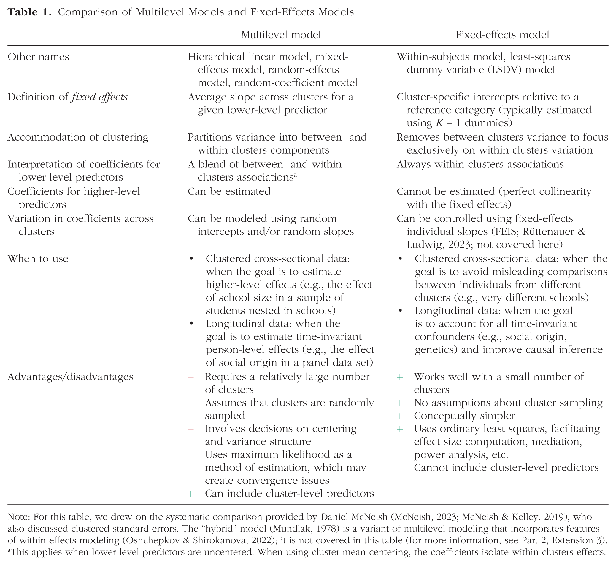
Note: For this table, we drew on the systematic comparison provided by Daniel McNeish (McNeish, 2023; McNeish & Kelley, 2019), who also discussed clustered standard errors. The “hybrid” model (Mundlak, 1978) is a variant of multilevel modeling that incorporates features of within-effects modeling (Oshchepkov & Shirokanova, 2022); it is not covered in this table (for more information, see Part 2, Extension 3).

This applies when lower-level predictors are uncentered. When using cluster-mean centering, the coefficients isolate within-clusters effects.

In Part 2, we expand on the concepts introduced in Part 1 to show how fixed-effects (panel) modeling applies to longitudinal analysis using a synthetic data set in which students are followed for 4 weeks and, again, we provide R, Stata, and SPSS scripts. The growing availability of large-scale panel surveys has become a valuable resource for psychologists because these data sets allow researchers to track individuals over time and study changes in psychological outcomes (Lillard, 2024). Major panel data sets—such as the German Socio-Economic Panel, the Swiss Household Panel, the U.S. Panel Study of Income Dynamics, and the Korean Labor and Income Panel Study—offer repeated measures relevant to psychology, including family dynamics, personality, and mental health (for a more exhaustive list of data sets, see Table A1 in the Appendix). Psychologists can use fixed-effects panel modeling (and its extensions) to examine associations among these measures while focusing only on within-persons change, thereby eliminating all participant confounders that do not vary over time (e.g., genetic dispositions, family social class, ethnicity) and offering a stronger basis for causal inference (e.g., Seifert et al., 2024).

In Part 3, we discuss the strengths and limitations of fixed-effects panel modeling and offer reflections on causality. Although other fields have long engaged with the challenge of drawing causal inferences from longitudinal data, psychological research has been more hesitant to address causality outside of experimental designs (Grosz et al., 2020). Fixed-effects models help approach causality by isolating within-persons change over time and removing all time-invariant confounders. However, time-varying confounding and reverse causation remain key threats to causal inference. We propose viewing causality not as a binary judgment but as a continuum of plausibility: Fixed-effects panel modeling leverages within-persons variation in longitudinal data and raises the plausibility of causal inference beyond that of cross-sectional analyses even if these models cannot establish causality with certainty.

Part 1: Fixed-Effects Modeling Applied to Clustered Cross-Sectional Data

In this section, we show how fixed-effects modeling can be used to estimate within-clusters associations in cross-sectional data. Imagine you have collected a sample of N = 200 students across K = 4 schools (your four clusters). Students reported the number of hours they spent on sports activities in the previous week (your predictor). Then, they completed a depression screening tool and received a depression score ranging from 0 to 5 (your outcome). Your hypothesis is the following: “The more students do sports, the less depressed they are.”¹

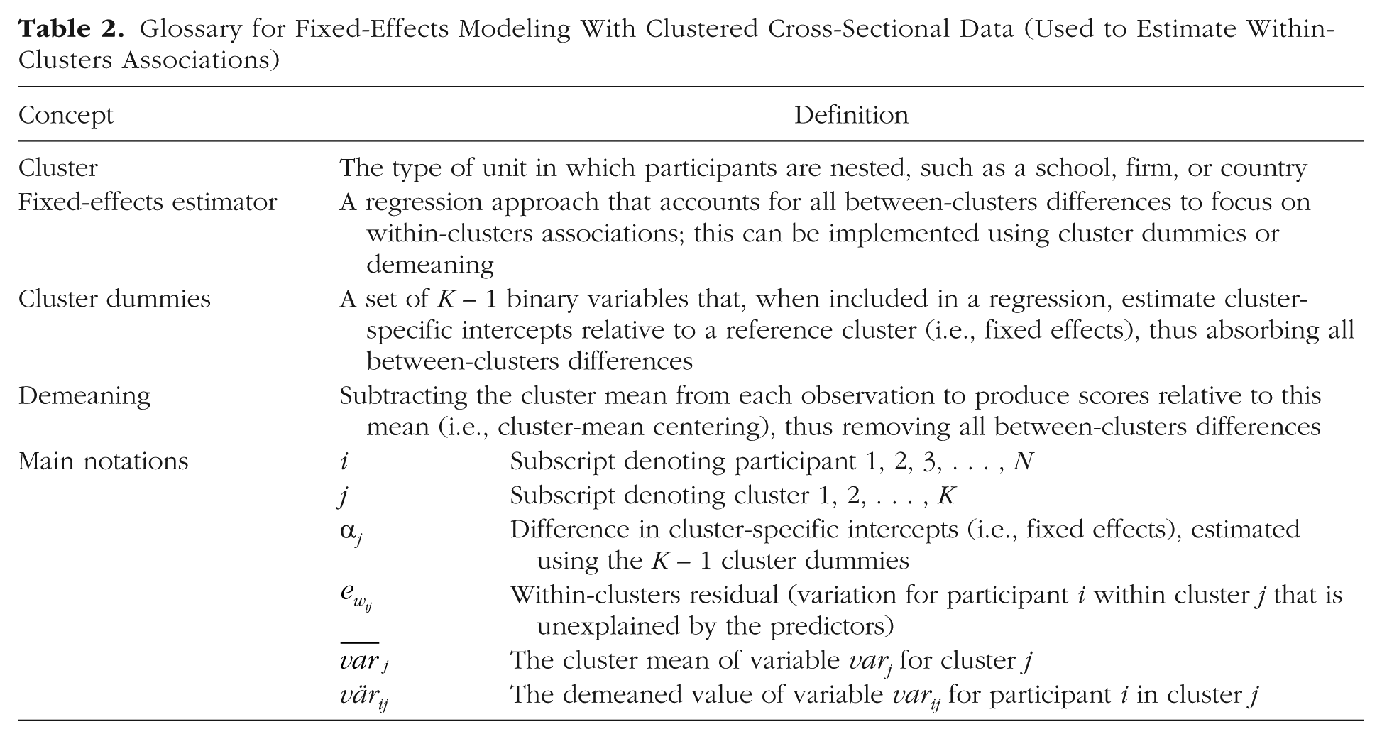
Here, we go through four modeling strategies to pedagogically explain how fixed-effects modeling works and how it can be used to estimate the within-schools association between sports and depression: (a) a standard regression, (b) a regression with cluster dummies, (c) a regression with demeaned variables, and (d) a fixed-effects regression with R, Stata, and SPSS. The synthetic clustered data set and the Quarto (R), Stata, and SPSS scripts to run the analyses are available at https://osf.io/fvck7/. We encourage you to work with these resources while reading this section. Table 2 is a glossary of concepts and notation used throughout this section, and Box 1, at the conclusion of the section, provides a concise summary.

Table 2.

Glossary for Fixed-Effects Modeling With Clustered Cross-Sectional Data (Used to Estimate Within-Clusters Associations)

Concept	Definition
Cluster	The type of unit in which participants are nested, such as a school, firm, or country
Fixed-effects estimator	A regression approach that accounts for all between-clusters differences to focus on within-clusters associations; this can be implemented using cluster dummies or demeaning
Cluster dummies	A set of K – 1 binary variables that, when included in a regression, estimate cluster-specific intercepts relative to a reference cluster (i.e., fixed effects), thus absorbing all between-clusters differences
Demeaning	Subtracting the cluster mean from each observation to produce scores relative to this mean (i.e., cluster-mean centering), thus removing all between-clusters differences
Main notations	i	Subscript denoting participant 1, 2, 3, . . . , N
	j	Subscript denoting cluster 1, 2, . . . , K
	α_j	Difference in cluster-specific intercepts (i.e., fixed effects), estimated using the K – 1 cluster dummies
	$e_{w_{i j}}$	Within-clusters residual (variation for participant i within cluster j that is unexplained by the predictors)
	${\bar{v a r}}_{j}$	The cluster mean of variable var_j for cluster j
	vär_ij	The demeaned value of variable var_ij for participant i in cluster j

Box 1. Summary of Part 1

• Fixed-effects modeling is a simple and effective approach to account for data clustering in cross-sectional data and to isolate within-clusters associations between variables.

• Fixed-effects modeling can be implemented by including the cluster identifier as a categorical predictor (Model 2), which fully removes between-clusters variation.

• Fixed-effects modeling can also be implemented by demeaning the focal predictor and outcome (Model 3), although degrees of freedom must be corrected for mean estimation.

• Fixed-effects modeling can be implemented using R (plm()), Stata (xtreg, fe), and SPSS (UNIANOVA), respectively (Model 4); full commands are provided in the text.

Model 1: standard regression

First, you run this standard regression model:

d e p r e s s i o n_{i j} = B_{0} + B_{1} \times s p o r t_{i j} + e_{i j},

(1)

where i = 1, 2, . . . , 200 participants; j = 1, 2, 3, 4 schools; B₀ is the intercept (the predicted depression score for respondents who did not do sports in the prior week); and e_ij is the residual.

Note that in Equation 1 and the following regression equations, the residuals are assumed to satisfy the basic regression assumptions: normally distributed, e_ij ∼ N(0, σ²); homoscedastic, Var(e_ij | sport_ij) = σ²; and independent (for a discussion of when clustering needs to be taken into account, see the section on “Design Effect” in Sommet & Morselli, 2021).

As shown in Table 3, your estimate of interest is B₁ = −0.01, SE = 0.07, p = .913. You may believe it accurately captures the association between doing sports and depression. However, this estimate is biased for two reasons. First, using a standard regression with a clustered data set violates the independence assumption, which requires that residuals associated with different participants be independent of one another (Snijders & Bosker, 2012). In your case, this assumption does not hold because data from students from the same school are likely more similar than data from students from different schools.

Table 3.

Parameters From the Four Modeling Strategies Presented in Part 1

Model 1: standard regression^a	B	SE	p	← 198 residual df (N – 2 estimated parameters)
Intercept, B₀	2.65	0.25	< .001	← Mean depression score for students not doing sports
Number of hours devoted to sports, B₁	−0.01	0.07	0.913	← Overall effect for students from similar and different schools (biased)
var(e_ij)	1.735			← Overall residual variance
Model 2: regression with cluster dummies^b	B	SE	p	← 195 residual df (N – 2 – 3 school dummies)
Intercept, α₀	5.40	0.13	< .001	← Mean depression score for students not doing sports in school S1^e
Number of hours devoted to sports, B₁	−0.26	0.03	< .001	← Pooled within-schools association between sports and depression (unbiased)
School dummies
School S1 vs. School S2, α₁	−1.34	0.08	< .001	← Difference between intercepts in School S1 and School S2^e
School S1 vs. School S3, α₂	−3.51	0.07	< . 001	← Difference between intercepts in School S1 and School S3^e
School S1 vs. School S4, α₃	−2.57	0.09	< .001	← Difference between intercepts in School S1 and School S4^e
$v a r (e_{w_{i j}})$	0.107			← Within-schools residual variance
Model 3: regression with demeaned variables^c	B	SE	p	← 198 residual df (N – 2 estimated parameters)
Intercept	0.00	0.02	1.000	← Not informative because demeaning results in a value of zero
Number of hours devoted to sports, B₁	−0.26	0.02	< .001	← Pooled within-schools association between sports and depression (standard error and p-value are biased)
var(ë_ij)	0.106			← Within-schools residual variance
Model 4: fixed-effects regression (software output)^d	B	SE	p	← 195 residual df (N – 2 – 3 estimated cluster means)
Intercept	n/a	n/a	n/a	← Not estimated because demeaning results in a value of zero
Number of hours devoted to sports, B₁	−0.26	0.03	< .001	← Pooled within-schools association between sports and depression (unbiased)
var( $e_{w_{i j}})$ or var(ë_ij)	0.107			← Within-schools residual variance

Note: Results shown are from the standard regression, regression with cluster dummies, regression with demeaned variables, and fixed-effects regression run using your preferred software. The latter three models yield the pooled within-clusters association between the predictor and outcome, as described by the text in bold.

This model is biased because it violates the independence assumption and fails to isolate within-clusters associations.

This model is unbiased and is a fixed-effects model.

This model isolates within-clusters associations, but the standard errors are biased because it ignores the degrees of freedom used to estimate cluster means. The bias is minimal here because our example uses K = 4 schools for easier graphical display, but it would grow with K = 10, 20, or more schools.

This model is unbiased and can be replicated using the R, Stata, and SPSS commands described in the text.

This estimate is generally neither interpreted nor reported in fixed-effects-regression results.

Second, using a standard regression with a clustered data set fails to isolate the within-clusters associations because estimates reflect differences not only among participants in the same clusters but also across different clusters (Enders & Tofighi, 2007). In your case, treating students from different schools as interchangeable units can lead to misleading comparisons. Does it really make sense to estimate the association between sports participation and depression by comparing students in less affluent versus more affluent schools, rural versus urban schools, or regular schools versus schools with elite sports programs? A more defensible strategy is to compare each student with peers from the same school, thereby isolating the within-schools association.

There are various tools for addressing the violation of the independence assumption (e.g., clustered standard errors; Cameron & Miller, 2015) and isolating within-clusters associations (e.g., cluster-mean centering in multilevel modeling; Bell et al., 2018). However, fixed-effects modeling arguably stands out as the simplest solution for modeling within-clusters associations.

Model 2: regression with cluster dummies

Second, you run the same regression as in Equation 1 but add school dummies:

\begin{array}{l} d e p r e s s i o n_{i j} = B_{1} \times s p o r t_{i j} + α_{0} + α_{1} \times S 1 v s S 2 \\ + α_{2} \times S 1 v s S 3 + α_{3} \times S 1 v s S 4 + e_{w_{i j}}, \end{array}

(2)

where i = 1, 2, . . . , 200 participants; j = 1, 2, 3, 4 schools; and $e_{w_{i j}}$ is the within-schools residual.

In this model, you essentially treat school identifiers as a categorical variable. You include K – 1 = 3 dummy-coded variables in Equation 2, with School S1 serving as the arbitrary reference category. This means that (a) α₀ represents the mean depression score in School S1 when sport_i₁ = 0 (the intercept in School S1), (b) α₁ contrasts this score with the intercept in School S2, (c) α₂ contrasts it with the intercept in School S3, and (d) α₃ contrasts it with the intercept in School S4.² This approach is referred to as the “least-squares dummy variable” (LSDV) model (Brüderl & Ludwig, 2015) and can be written more simply as follows:

d e p r e s s i o n_{i j} = B_{1} \times s p o r t_{i j} + α_{j} + e_{w_{i j}} .

(2′)

In the context of fixed-effects modeling, the intercept α₀ and the K – 1 cluster-dummy coefficients (α₁ to α_K–1) are collectively referred to as “fixed effects” and denoted by α_j . Fixed effects are generally not interpreted, although researchers may inspect them to examine cluster-specific patterns in the outcome (e.g., which school has the highest intercept or to create the regression line for a particular school). In practice, the primary function of the fixed effects is to account for all unobserved differences between clusters. Simply put, by using school dummies, your model becomes fully saturated at the cluster level, leaving no between-schools differences to be explained. Thus, if you were to add a school-related variable as an additional predictor (e.g., school size, school resources), its effect could not be estimated because all between-schools variation is already accounted for. This addresses the violation of the independence assumption (McNeish & Kelley, 2019).³

As shown in Table 3, your estimate of interest is now B₁ = −0.26, SE = 0.03, p < .001. In this model, B₁ is uncontaminated by between-clusters differences because these are accounted for by the inclusion of cluster dummies. Therefore, B₁ is interpreted as the pooled within-schools association between doing sports and depression. To be clear, students are compared only with their schoolmates (e.g., students from School S1 are compared only with their peers in School S1), meaning that B₁ reflects the within-schools association based on comparisons made within each school and aggregated across schools. Following the same principle, the error term is now denoted $e_{w_{i j}}$ and represents the within-schools residual. This approach effectively addresses the problem of isolating within-clusters associations. However, although this LSDV model is a fixed-effects model, the same result can be obtained using a technique that is perhaps more common in practice: demeaning.

Model 3: regression with demeaned variables

Third, you run the same regression as in Equation 1 but first subtract the mean of each school from each individual observation:

(d e p r e s s i o n_{i j} - {\bar{d e p r e s s i o n}}_{j}) = B_{1} \times (s p o r t_{i j} - {\bar{s p o r t}}_{j}) + (e_{i j} - {\bar{e}}_{j}),

(3)

where the diacritical lines (the bars) denote the school-specific mean (four possible values).

By subtracting the relevant cluster mean from each individual observation, you generate values that are relative to that cluster mean. For instance, (a) a negative score on the demeaned depression variable indicates that the student is less depressed than the student’s schoolmates (e.g., −2 means the student is 2 points less depressed than the school average), (b) a null score indicates that the student is as depressed as the student’s schoolmates (i.e., 0 means the student matches the school average), and (c) a positive score indicates that the student is more depressed than the student’s schoolmates (e.g., +2 means the student is 2 points more depressed than the school average). This procedure is known as “demeaning” (Wooldridge, 2010) and is similar to cluster-mean centering in multilevel modeling (Bell et al., 2018; Enders & Tofighi, 2007; Hamaker & Muthén, 2020). The equation can be written more simply as follows:

\overset{\cdot\cdot}{d e p r e s s i o n_{i j}} = B_{1} \times \overset{\cdot\cdot}{s p o r t_{i j}} + e_{w_{i j}},

(3′)

where the diacritical marks (the dots) indicate that the variable has been demeaned.

As illustrated by Figure 1, after demeaning your predictor and outcome, each school ends up with an average sport time and depression score of zero. In Figure 1 (left), the uncentered variables suggest that School S1 has higher averages in both sport time and depression (perhaps this is an elite sports school where students feel intense pressure), whereas School S4 has a higher average for sport time and a lower average for depression (perhaps this is a private school with more resources). As also shown in Figure 1 (middle, right), demeaning aligns the averages for both predictor and outcome across schools, thereby removing all between-schools differences.

Fig. 1.

Graphical representation of the demeaning procedure. Shown are school-specific regression lines with (left) uncentered variables, (middle) demeaned outcome, and (right) demeaned outcome and predictor (as in fixed-effects modeling). School S1 (red filled circles) may be a competitive athletic school where students are under performance pressure, resulting in high levels of sports activity but also a high risk of depression, whereas School S4 (green triangles) may be a private school with greater resources to offer sports activities and a student body from wealthier families, resulting in high levels of sports activity and a low risk of depression. (Left) The black dashed line represents the standard regression line ignoring school clustering, B₁ = −0.01, SE = 0.07, p = .913 (Model 1). (Right) The black dashed line represents the fixed-effects regression line, B₁ = −0.26, SE = 0.03, p < .001 (Models 2 and 4).

As shown in Table 3, your estimate of interest is B₁ = −0.26, SE = 0.02, p < .001. The coefficient estimate is identical to that of the regression using cluster dummies. The reason is that it is also uncontaminated by between-clusters differences because these have been eliminated through demeaning. The coefficient estimate is again interpreted as the pooled within-schools association between doing sports and depression. Note that the model no longer requires an intercept because it is effectively zero, and that $e_{w_{i j}}$ —which could also be denoted ë_ij—again represents the within-schools residual.

However, the standard error—and by extension, the inferential test, confidence interval, and p value—differ from that in the regression using cluster dummies. The reason is that demeaning was performed manually, without accounting for the degrees of freedom consumed by the estimation of cluster means (Judge et al., 1991). Consequently, the standard error is slightly underestimated, although the bias is minor because we have only K = 4 clusters (i.e., only K – 1 = 3 df are unaccounted for). The discrepancy will become larger as K increases, which can lead to erroneous conclusions (e.g., if the 200 students had been drawn from 50 schools). This issue will be resolved by your statistical software.

Model 4: fixed-effects regression using R, Stata, and SPSS

Finally, you run a fixed-effects regression using your favorite software:

R summary(plm(depression ~ sport, data = df_clustered, index = "school_id", model = "within"))

Stata xtreg depression sport, fe i(school_id)

SPSS UNIANOVA depression BY school_id WITH sport /INTERCEPT=EXCLUDE /PRINT PARAMETER.

where depression is the outcome, sport the predictor, and school_id the school identifier. R users should install the package plm (Croissant & Millo, 2008). Stata users should note that xtreg, fe reports an intercept, which is not directly estimated but represents the average of the fixed effects (i.e., the mean school-specific intercept).

Technically, both plm() with model = “within” in R and xtreg, fe in Stata use demeaning while appropriately accounting for the degrees of freedom consumed by the estimation of cluster means, yielding the same residual degrees of freedom as the regression with cluster dummies (SPSS does not have a built-in command for fixed-effects modeling, and we run a regression with cluster dummies). Regardless, you can describe your model using either Equation 2′ (using cluster-dummy notation) or Equation 3′ (using demeaning notation).

As shown in Table 3, your estimate of interest is B₁ = −0.26, SE = 0.03, p < .001. This finding supports your hypothesis: Students in a given school who reported 1 additional hour of sports activity relative to their schoolmates scored, on average, a quarter of a point lower on the depression-screening tool. Note that built-in fixed-effects routines in R or Stata return the same focal coefficient estimates and standard errors as a regression with cluster dummies because both approaches are fixed-effects models that focus exclusively on within-clusters variation. Either approach can be used for estimation, although the output from the regression with school dummies may be tedious to read when there are many clusters because it displays the K – 1 fixed effects.

Comparing fixed-effects and multilevel modeling for clustered cross-sectional data

Fixed-effects modeling is an elegant and practical approach for estimating the pooled within-clusters association between two variables in clustered cross-sectional data. Although psychologists often default to multilevel modeling for such analyses, fixed-effects modeling offers several advantages (see Table 1). For instance, fixed-effects modeling performs relatively well with a small number of clusters (even with K = 4, as in our example; Maas & Hox, 2005; McNeish & Stapleton, 2016) and does not require clusters to be sampled from a representative population of clusters (Bryan & Jenkins, 2015).⁴ Note, however, that regardless of modeling strategy, a small or nonrepresentative set of clusters limits the generalizability of the findings (Firebaugh, 2018). Moreover, although multilevel modeling relies on complex maximum-likelihood optimization methods, fixed-effects modeling uses ordinary least squares, which is more efficient, does not create convergence problems, and makes it simpler to calculate residual-based effect sizes (Olejnik & Algina, 2003) or conduct 1-1-1 mediation analysis (Hayes, 2013).⁵ Despite these advantages, fixed-effects modeling has an important drawback: By focusing exclusively on within-clusters variation, it cannot estimate the main effects of cluster-level predictors. Multilevel modeling therefore remains necessary when the research question concerns between-clusters differences.

Beyond the choice of model, concluding that doing sports leads to reduced depression based on your data would be misguided. Psychologists often overlook a fundamental assumption in regression: exogeneity (Gardiner et al., 2009). This assumption requires that regressors be uncorrelated with the residual, which is a sophisticated way of saying that your focal predictor must be a true independent variable, unaffected by between-participants confounders (for a discussion, see Maxwell et al., 2017, p. 62). Although your fixed-effects model removes all between-schools sources of noise, it does not address more critical threats to causal inference, such as time-invariant person-level confounders (Pearl, 2009). Addressing such concerns requires longitudinal analysis.

Part 2: Fixed-Effects Modeling Applied to Longitudinal Data

In this section, we show how fixed-effects modeling can be used to estimate within-participants associations in longitudinal data. Imagine you have followed N = 800 undergraduates over the course of T = 4 weeks (yielding a total of 800 × 4 = 3,200 within-participants observations). Each week, students recorded the number of hours they spent on sports activities (your predictor, with four data points per participant) and completed the same depression-screening tool used in the cross-sectional study (your outcome, with four data points per participant). Your hypothesis is the same as before: “The more students do sports, the less depressed they are.”

Part 2 builds on the concepts presented in Part 1 (fixed-effects estimator, cluster dummies, demeaning) to focus on the most critical application of fixed-effects modeling: longitudinal data. Here, we begin by showing how the classical two-way fixed-effects panel model can be used to estimate the within-participants association between sports and depression over time. Next, we show how to estimate two types of interaction that involve different combinations of time-invariant and time-varying predictors. Finally, we introduce three extensions: (a) first-difference modeling, (b) time-distributed fixed-effects modeling, and (c) within-between multilevel modeling. The synthetic longitudinal data set and the Quarto (R), Stata, and SPSS scripts to run the analyses are available at https://osf.io/7mz2q/. We encourage you to work with these resources while reading this section. Table 4 provides a glossary of the jargon and notation used in this section.

Table 4.

Glossary for Fixed-Effects Panel Modeling With Longitudinal Data (Used to Estimate Within-Persons Associations)

Concept	Definition
Fixed-effects estimator	A regression approach that accounts for all time-invariant between-participants differences to focus exclusively on within-participants variation; this can be implemented using participant dummies or demeaning
Participant dummies	A set of N – 1 binary variables that when included in a regression, estimate participant-specific intercepts relative to a reference participant (i.e., participant fixed effects), thus absorbing all time-invariant between-participants differences
Demeaning	Subtracting the participant mean from each observation to produce change scores (i.e., person-mean centering), thus removing all time-invariant between-participants differences
Panel-adjusted standard errors	A variance estimator that makes standard errors robust to violations typical in panel data (cluster-robust)
Detrending	Removing time trends in longitudinal data by statistically controlling for the linear effect of time
Time fixed effects	A set of time dummies used to eliminate all between-waves differences and produce estimation net of period effects
Two-way fixed effects	A fixed-effects panel model that includes both participant and time fixed effects
Time-invariant variable	A trait-like participant feature that does not vary over time (e.g., biological sex at birth, family social class)
Time-varying variable	A state-like participant feature that varies over time (e.g., income, health)
Double demeaning	Subtracting the participant mean from variables X and W, forming the product X × W, and subtracting the participant mean of X × W
Main notations	i	Subscript denoting participant 1, 2, 3, . . . , N
	t	Subscript denoting Wave 1, 2, . . . , T
	α_i	Difference in participant-specific intercepts (i.e., participant fixed effects), estimated using N – 1 dummies
	λ_t	Difference in time-specific intercepts (i.e., time fixed effects), estimated using T – 1 dummies
	$e_{w_{i t}}$	Within-participants residual (variation for participant i at time t that is unexplained by the predictors)
	${\bar{v a r}}_{i}$	The participant mean of a variable var for a participant i
	vär_it	The demeaned value of variable var_it for participant i at time t (person-mean-centered value)

Fixed-effects panel regression

If you analyzed the relationship between sports and depression using a standard regression model, time-invariant individual differences—such as temperament, athletic predisposition, or chronic health conditions—could bias the estimates. For instance, students with greater baseline stamina may be both more likely to engage in sports and less likely to feel depressed even if sports itself has no causal effect on depression. The model would then mistakenly attribute these stable, unmeasured differences to the effect of sports.

Fixed-effects modeling applied to longitudinal data addresses this issue by removing all time-invariant between-persons differences from the estimation. The principles are similar to those described in Part 1 with one key difference: The clusters are now the participants themselves rather than higher-level units, such as schools (Allison, 2009; Brüderl & Ludwig, 2015; Wooldridge, 2010). In this context, the model is called a “fixed-effects panel model” and can again be conceptualized in two ways.

Regression with participant dummies

A fixed-effects panel model can be conceptualized as a regression that includes participant identifiers as a categorical variable (akin to Model 2 in Part 1). In practice, this entails incorporating N – 1 dummy variables (whose coefficients are referred to as “fixed effects”) so that all time-invariant differences are absorbed and no stable between-participants variation is left to be explained. The model therefore focuses exclusively on within-participants change.

Regression with demeaned variables

A fixed-effects panel model can also be conceptualized as a regression that uses demeaned outcomes and predictor(s) (akin to Model 3 in Part 1). In practice, this entails subtracting the participant-specific mean from each observation (also known as “person-mean centering”). After this transformation, a positive value on sports, for example, marks a moment when the student is more active than usual, whereas a negative value on depression marks a moment when the student feels less depressed than usual. As before, any association between two variables now reflects within-participants change.

Both models are fixed-effects panel models and will produce identical slope estimates, although in the demeaned specification, the degrees of freedom must be adjusted to account for the estimation of participant means (Judge et al., 1991). Before explaining how to run this model, we consider two precautions.

Precaution 1: using panel-adjusted standard errors

Scholars have pointed out that fixed-effects panel modeling does not automatically address the problem of nonindependent residuals in longitudinal data (Arellano, 1987; McNeish & Kelley, 2019). Consequently, many researchers have advocated for the use of panel-adjusted standard errors (Angrist & Pischke, 2009; Brüderl & Ludwig, 2015; MacKinnon et al., 2023), which accommodate arbitrary heteroskedasticity (unequal residual variances) and serial correlation (dependence of residuals over time) within participants (MacKinnon et al., 2023). In the remainder of this primer, we systematically incorporate panel-adjusted standard errors in our R, Stata, and SPSS commands (Cameron & Miller, 2015).

Note that default CR1-type panel-adjusted standard errors can be biased in samples smaller than N ≈ 50 participants (Kézdi, 2004), and other cluster-robust variance estimators (e.g., CR2) have been proposed (Pustejovsky & Tipton, 2018). Alternatively, analysts can use feasible generalized least squares (FGLS), an estimation method that directly models the assumed serial correlation in the residuals rather than merely correcting the standard errors (Bai et al., 2021). Although potentially more efficient, FGLS requires correctly specifying the error covariance structure and is not supported in all statistical software.⁶ Even more complex approaches, such as alternative variance formulas and bootstrap procedures, have also been proposed (Abadie et al., 2023).

Precaution 2: taking time into account

Another important consideration when analyzing longitudinal data is the inclusion of time in the model. There are two main strategies here. First, time can be treated as a continuous covariate. This approach, often referred to as “detrending the time-varying outcome,” conceptualizes time as a linear confounder (Wang & Maxwell, 2015). It enables analysts to partial out the variance attributable to the passage of time (Hoffman & Stawski, 2009; for a more in-depth discussion, see Falkenström et al., 2023). Second, time can be treated as a categorical covariate. This approach, known as “two-way fixed-effects panel modeling,” incorporates both participant fixed effects (e.g., using participant dummies) and time fixed effects (e.g., using time dummies; Wooldridge, 2021). It enables analysts to isolate the estimates of interest net of period effects (Kropko & Kubinec, 2020). Technically, in such a model, observations are treated as cross-classified by participants and periods. Although two-way fixed-effects panel modeling has been criticized for creating interpretational complexities (Hill et al., 2020; Imai & Kim, 2021), it is a common strategy to account for time, and we use it throughout the remainder of this primer.

Implementing a two-way fixed-effects panel model in R, Stata, and SPSS

In the conceptualization of fixed-effects modeling using participant dummies to focus on within-persons variation, the two-way fixed-effects panel modeling equation is as follows:

d e p r e s s i o n_{i t} = B_{1} \times s p o r t_{i t} + α_{i} + λ_{t} + e_{w_{i t}},

(4)

where i = 1, 2, . . . , 800 participants; t = 1, 2, 3, 4 waves; α_i are participant fixed effects (estimated using the N – 1 dummies); $λ_{t}$ are time fixed effects (estimated using the T – 1 dummies); and $e_{w_{i t}}$ is the within-participants residual.

In the conceptualization of fixed-effects modeling using demeaning to focus on within-persons variation, the two-way fixed-effects panel modeling equation is as follows:

\overset{\cdot\cdot}{d e p r e s s i o n_{i t}} = B_{1} \times \overset{\cdot\cdot}{s p o r t_{i t}} + λ_{t} + e_{w_{i t}},

(5)

where the diacritical marks (the dots) indicate that the variable has been demeaned (with standard errors adjusted for the degrees of freedom used to estimate participant means).

Equations 4 and 5 are equivalent. Below are the relevant commands in your preferred software with panel-adjusted standard errors:

plm(depression ~ sport, data = df_longitudinal, index = c("part_id", "wave"), model = "within", effect = "twoways") %>% coeftest(., vcovHC(., type = "HC1", cluster = "group"))

Stata xtreg depression sport i.wave, fe i(part_id) vce(cluster part_id)

SPSS UNIANOVA depression BY part_id wave WITH sport /INTERCEPT=EXCLUDE /PRINT PARAMETER /ROBUST=HC1 /DESIGN=part_id wave sport.

where depression is the outcome, sport is the predictor, part_id is the participant identifier, and wave is the time identifier. R users should install lmtest (Hothorn et al., 2015). The SPSS command addresses only heteroskedasticity. A CR1-based version is included in the script on the OSF but runs slowly as N increases.

Running either of these commands, you will find that your estimate of interest is B₁ = −0.31, SE = 0.02, p < .001. Figure 2 provides a graphical representation of this finding, showing the individual associations between the demeaned variables for the first eight participants for illustrative purposes. This finding supports your hypothesis: For each additional hour of sports activity per week, the depression score of a given participant decreases by a third of a point. Note that this estimate is free from what economists and sociologists have referred to as “time-constant individual heterogeneity” (Brüderl & Ludwig, 2015, p. 328). The fixed-effects estimator accounts for all observed and unobserved participant characteristics that do not vary over time, thereby removing any potential time-invariant confounders (i.e., variables assumed to be stable over time and to influence both the predictor and outcome variables; see Murayama & Gfrörer, 2024).

Fig. 2.

Within-participants association in a fixed-effects panel model. Shown are the pooled associations between sports and depression (solid line) with the 95% confidence interval (shaded area) and individual associations for the first eight participants (dashed lines).

Calculation of effect sizes and simulation-based statistical power

As mentioned previously, effect sizes in fixed-effects modeling can be calculated in the same way as in standard linear regression. For example, the partial eta square, which quantifies the proportion of within-individuals variance explained by a dichotomous or continuous predictor, can be calculated using the following formula (Cohen, 1965):

η_{p}^{2} = \frac{{(B \div S E)}^{2}}{{(B \div S E)}^{2} + d f_{r e s i d u a l}},

(6)

where df_residual represents the degrees of freedom for the residuals, calculated as the number of observations minus the number of estimated fixed effects and the number of predictors.

What constitutes a “typical” effect size in psychology? Gignac and Szodorai (2016) collected 708 meta-analytic correlations from psychological studies using cross-sectional designs and found that the 25th, 50th, and 75th percentiles of the distribution for between-participants effect sizes were η_p² ≈ .01 (smaller estimate), η_p² ≈ .04 (median estimate), and η_p² ≈ .08 (larger estimate), respectively.⁷ However, these benchmarks refer to between-persons effects and therefore do not automatically generalize to within-persons effects. Between-persons differences can span nearly the full response scale (e.g., 1–7 on a Likert item), whereas within-persons fluctuations are typically narrower (e.g., ±1 around the person mean), meaning that within-persons effect sizes may often be smaller (Hoffman & Stawski, 2009). To date, no systematic investigation has mapped the distribution of within-persons effect sizes from fixed-effects panel models to empirically assess this expectation (for research focused on cross-lagged panel models [CLPMs], see Orth et al., 2024). Nonetheless, illustrative findings suggest that such within-persons effects may often fall in the lower quartile of Gignac and Szodorai’s distribution, such as the within-persons associations between social media use and distraction (Siebers et al., 2022), loneliness and life satisfaction (Mader & Franzen, 2025), or financial scarcity and depression (Sommet & Spini, 2022).

Accordingly, we ran simulations to determine the sample size required to detect a within-persons association of η_p² ≈ .01 with 80% power and α = .05. We simulated 2,000 data sets for each of 50 sample sizes in three-, four-, and five-wave designs and identified the sample size at which 80% of the data sets produced a significant within-persons estimate in a one-way fixed-effects panel model. The simulations yielded three key findings: (a) N = 381 participants are required to detect a within-participants effect of η_p² ≈ .01 in a three-wave panel data set, (b) N = 259 are required in a four-wave panel data set, and (c) N = 192 are required in a five-wave panel data set (for the power curve and further details, see Fig. 3). These figures should be viewed as illustrative rather than prescriptive. The simulations assumed ideal conditions: balanced data with complete cases (i.e., no attrition and no item nonresponse), homogeneous within-persons slopes, and variation in the focal variables for all participants (for details, see the Limitations section). Moreover, expected effect sizes vary by subdiscipline, population, measurement, and other study characteristics (Schäfer & Schwarz, 2019). For instance, η_p² ≈ .01 is plausible in long-term longitudinal survey data (e.g., a yearly panel study), but the same estimates may not apply to repeated-measures experiments, which tend to show stronger effects (Flora, 2020; Onwuegbuzie & Levin, 2003; Sommet et al., 2023).

Fig. 3.

Power curves for detecting a within-persons association of η_p² ∼ .01 using fixed-effects panel modeling with T = 3, 4, and 5 waves. These power curves were derived from simulations in which $\bar{X}$ ∼ N (0, 1) and $\bar{Y}$ ≈ N (0, 1), with β_{(..Xit, ..Yit)} = 0.10 (η_p² ≈ .01) and ε_ij ∼ N(0, 1). For each curve, we began by simulating 2,000 data sets with sample size N = 100 and then increased N in increments of 10 until we identified the tipping points at which more than 80% of the data sets yielded a significant effect (α = .05) using a one-way fixed-effects panel model with panel-adjusted standard errors. Following earlier simulations (e.g., Yang et al., 2022), we set the intraclass correlation coefficient (ICC) to .50. However, because the proportion of within-persons variance explained by ..X_it was fixed to η_p² ≈ .01, the ICC does not affect the results.

Interaction effects in fixed-effects panel regression

Fixed-effects panel modeling allows analysts to test two types of second-order interactions: (a) the interaction between a time-invariant predictor and a time-varying predictor and (b) the interaction between two time-varying predictors.

Type 1: interaction between a time-invariant predictor and a time-varying predictor

Fixed-effects panel modeling cannot be used to estimate the statistical effects of a time-invariant predictor because the participant fixed effects leave no time-invariant differences between participants to be explained (Hsiao, 2022). However, it can be used to estimate whether the within-participants effect of a time-varying variable depends on a time-invariant participant characteristic (Allison, 2009). In multilevel modeling, this would be referred to as “cross-level interactions” (Aguinis & Gottfredson, 2010). For example, here is how to test whether the association between sports and depression over time varies between men (coded −0.5) and women (coded +0.5)⁸ :

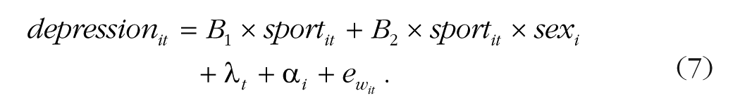
\begin{array}{l} d e p r e s s i o n_{i t} = B_{1} \times s p o r t_{i t} + B_{2} \times s p o r t_{i t} \times s e x_{i} \\ + λ_{t} + α_{i} + e_{w_{i t}} . \end{array}

(7)

Running the OSF-uploaded script for Equation 7, we find that the interaction term is B₂ = −0.01, SE = 0.05, p = .907. This indicates that the pooled within-participants association between sports and depression over time does not significantly differ between men and women. Equation 7 does not include the main effect of sex because—as with any time-invariant predictor—it cannot be estimated.

Type 2: interaction between two time-varying predictors

Fixed-effects panel modeling can also be used to estimate whether the within-participants effect of a time-varying variable varies as a function of another time-varying variable (Schunck, 2013). However, if you test such interactions using participant dummies or the demeaned product term of the nondemeaned variables (as your software typically does), the estimation will be contaminated by between-participants differences (Giesselmann & Schmidt-Catran, 2022). To mitigate this bias, one should use “double demeaning”: One should demean the product term of the already demeaned predictors to ensure accurate estimation of the pooled within-participants interaction term (Balli & Sørensen, 2013). For example, you can test whether the association between sports and depression over time varies as a function of sleep quality during the week of data collection:

\begin{array}{l} \overset{\cdot\cdot}{d e p r e s s i o n_{i t}} = B_{1} \times \overset{\cdot\cdot}{s p o r t_{i t}} + B_{2} \times \overset{\cdot\cdot}{s l e e p_{i t}} \\ + B_{3} \times \overset{\cdot\cdot}{\overset{\cdot\cdot}{s p o r t_{i t}} \times \overset{\cdot\cdot}{s l e e p_{i t}}} + λ_{t} + e_{w_{i t}}, \end{array}

(8)

where the diacritical marks denote demeaned variables and the stacked diacritical marks denote double demeaning with $\overset{\cdot\cdot}{\overset{\cdot\cdot}{s p o r t_{i t}} \times \overset{\cdot\cdot}{s l e e p_{i t}}} = \overset{\cdot\cdot}{s p o r t_{i t}} \times \overset{\cdot\cdot}{s l e e p_{i t}} - \overset{\cdot\cdot}{s p o r t_{i t}} \times \overset{\cdot\cdot}{s l e e p_{i t}}$ .

Running the OSF-uploaded script for this equation, we find that the interaction term is B₃ = −0.07, SE = 0.02, p < .001. This indicates that the pooled within-participants association between sports and depression over time differs according to sleep quality. Decomposing this interaction reveals that the association is weaker in weeks when the participant has poorer than usual sleep, B_–1SD = −0.07, SE = 0.03, p = .047, and stronger when the participant has better than usual sleep, B_+1SD = −0. 23, SE = 0.03, p < .001. Note that the recommendation to use double demeaning is based on recent work (Giesselmann & Schmidt-Catran, 2022), and the methodological consensus on this issue may continue to evolve.

Three extensions of fixed-effects panel modeling

Below, we briefly introduce three extensions of fixed-effects panel modeling: (a) first-difference modeling, (b) time-distributed fixed-effects modeling, and (c) within-between multilevel modeling.

Extension 1: first-difference modeling

Whereas fixed-effects panel models estimate the long-term association between two variables across waves, first-difference models capture the short-term association between changes in a predictor and changes in an outcome from one wave to the next (Allison, 2009). When only T = 2 waves of data are available, a fixed-effects model is equivalent to a first-difference model (Schmidheiny, 2023; for an article on longitudinal analyses with two waves of data, see Johnson, 2005). Here is the equation:

Δ d e p r e s s i o n_{i t} = B_{1} \times Δ s p o r t_{i t} + e_{w_{i t}},

(9)

where i = 1, 2, . . . , 800 participants; t = 2, 3, 4 waves; Δ denotes the difference between the variable score at time t and t – 1; and $e_{w_{i t}}$ is the within-participants residual.

Running the OSF-uploaded script, we find that the focal estimate is B₁ = −0.31, SE = 0.03, p < .001.⁹ As illustrated by Figure 4 (left), this indicates that for each additional hour of sports activity in a given week compared with the previous week, the depression score of a given participant decreases by 0.31 points. Note that fixed effects (for participants and time) do not appear in Equation 9 because they cancel each other when the first differences are taken (Schmidheiny & Siegloch, 2023). Moreover, data from the first wave cannot be used because the initial value of the predictor or outcome is unknown (i.e., t = 2, 3, 4).

Fig. 4.

Associations of interest in (left) first-difference modeling, (middle) time-distributed fixed-effects modeling, and (right) within-between multilevel modeling. The figure shows (left) the associations between sports and depression from one wave to the next; (middle) the changes in depression scores before, during, and after beginning sports; and (right) the within-participants and between-participants associations between sports and depression (the 95% confidence intervals are indicated by the shaded areas or error bars).

Extension 2: time-distributed fixed-effects modeling

Whereas fixed-effects panel models estimate the gradual statistical effect of a continuous predictor, time-distributed fixed-effects models track changes in the outcome for each wave preceding or following a particular event (Ludwig & Brüderl, 2021). This approach—also known as “dummy impact functions”—is particularly popular for modeling anticipation effects (changes occurring before the event) and scarring effects (changes persisting after the event) in relation to events such as job loss, divorce, or the birth of a child (Clark et al., 2008). Technically, the predictor is replaced by a series of binary indicators, each representing a specific time point relative to the event (e.g., “2 weeks before,” “week of,” “1 week after”), allowing the model to freely estimate changes in the outcome at each time point (i.e., without imposing a linear form). In our example, we focus on the participants who started doing sports during the study, and we create binary indicators for the weeks before, during, and after they began:

\begin{array}{l} d e p r e s s i o n_{i t} = B_{1} \times T_{- 2_{i t}} + B_{2} \times T_{- 1_{i t}} + B_{3} \times T_{0_{i t}} \\ + B_{4} \times T_{+ 1_{i t}} + B_{5} \times T_{+ 2_{i t}} + α_{i} + e_{w_{i t}}, \end{array}

(10)

where i = 1, 2, . . . , 175 participants; t = 1, 2, 3, 4 waves; $T_{0_{i t}}$ is a binary variable coded 1 in the week the participant began sports (0 otherwise); $T_{\pm n_{i t}}$ is coded 1 in the nth week before/after the participant began sports (0 otherwise); and $e_{w_{i t}}$ is the within-participants residual.

Running the OSF-uploaded script, we find that B₁ and B₂ are null and that B₃ through B₅ are significantly negative. As illustrated by Figure 4 (middle), this indicates that a participant who starts doing sports during a given week experiences an immediate reduction in depression scores, which persists for at least 2 weeks. This analysis is confined to the subset of participants who started sports within the 4-week window of the study (i.e., n = 175 out of 800). Generally speaking, this analysis may exclude additional data points because some participants may experience multiple spells of activity (e.g., resuming sports after a break), and analysts often focus only on the initial spell.

Extension 3: within-between multilevel modeling

Whereas fixed-effects panel models focus solely on within-participants associations, within-between multilevel models are one of several hybrid approaches that simultaneously estimate within- and between-participants associations (e.g., Hamaker & Muthén, 2020; Kreft et al., 1995; Mundlak, 1978). These models are labeled “hybrid” because they combine features of both fixed-effects and multilevel models: As fixed-effects models, they use demeaning to capture relationships involving time-varying predictors; as multilevel models, they use a random intercept while modeling relationships involving time-invariant predictors (Brüderl & Ludwig, 2015). Specifically, the within-between multilevel model incorporates two distinct versions of the focal predictor: (a) the demeaned predictor (i.e., person-mean centered), which estimates the within-participants association, and (b) the person-specific predictor mean (i.e., a single value per participant), which estimates the between-participants association. Here is the equation:

\begin{array}{l} d e p r e s s i o n_{i t} = B_{00} + B_{w i t h i n} \times \overset{\cdot\cdot}{s p o r t_{i t}} + B_{b e t w e e n} \times {\bar{s p o r t}}_{i} \\ + λ_{t} + u_{0 i} + e_{w_{i t}} \end{array}

(11)

where the diacritical marks denote the demeaned predictor, the diacritical line denotes the person-specific mean, B₀₀ is the fixed intercept (mean outcome across participants), u_0i is the random intercept (between-participants residual), and $e_{w_{i t}}$ is the within-participants residual.

Running the OSF-uploaded script, we find that B_within = −0.31, SE = 0.02, p < .001 and B_between = −0.04, SE = 0.01, p < .001. As illustrated by Figure 4 (right), this indicates that (a) for each additional hour of sports per week, a given participant’s depression score decreases by 0.31 points, whereas (b) for each additional average weekly hour of sport, participants’ depression scores are 0.04 points lower compared with other participants. Note that B_within and its standard error match B₁ and SE₁ from the fixed-effects panel regression model (Equations 4 and 5). Because both estimates capture the within-participants association, they are expected to be identical, although minor decimal variations might occur because multilevel modeling uses maximum-likelihood estimation rather than ordinary least squares.

If you are interested in estimating both within- and between-participants associations for your focal variable(s), a within-between multilevel model is preferable to a fixed-effects panel model. However, if your interest lies solely in within-persons associations, each approach has its strengths and limitations. On the one hand, within-between multilevel models are highly flexible but rest on the distributional assumptions of multilevel modeling and require preliminary transformations to correctly separate within- and between-persons associations (Curran & Bauer, 2011). On the other hand, fixed-effects models are less versatile but involve minimal assumptions and yield coefficients that are directly interpretable as within-persons associations; they also rely on simple closed-form estimation procedures that are not subject to convergence issues and support direct extensions of standard regression techniques (Angrist & Pischke, 2009).

Limitations of fixed-effects modeling

Fixed-effects modeling is a straightforward and effective method for examining within-participants associations in longitudinal data while controlling for time-invariant confounders, thereby strengthening causal inference. Nevertheless, it has important limitations.

First, fixed-effects models assume slope homogeneity: All units are expected to share the same slope for any time-varying predictor (Hashem Pesaran & Yamagata, 2008). In the example above, our fixed-effects panel model estimates a separate intercept for each participant but constrains all individual sport-depression slopes to be parallel. When the assumption of slope homogeneity is violated, such a one-size-fits-all slope risks misattributing effects (Ludwig & Brüderl, 2018). Several diagnostics can be used to evaluate this assumption (e.g., Hausman-like tests), and the fixed-effects-individual-slopes (FEIS) approach can relax it by interacting the time-varying predictor with participant dummies, thereby giving individuals their own slope (Rüttenauer & Ludwig, 2023). Although FEIS reduces heterogeneity bias, it typically requires a very large sample size (Morgan & Winship, 2014).

Second, fixed-effects panel models often rely on an effective sample size that is smaller than the total sample size (Beck & Katz, 2001). Because these models focus on within-persons variation, participants who show no change over time do not contribute to slope estimation. In our example, only the subset of participants who move from active to inactive (or vice versa) and from depressed to not depressed (or vice versa) inform the results. Consequently, the analysis draws on fewer informative cases than the raw sample count suggests, reducing statistical power. It is therefore advisable to report the proportion of participants who exhibit within-persons variability, clarifying how many are involved in the analysis (Hill et al., 2020).

Finally, the two most important limitations affecting causal inference—time-varying confounders and reverse causation—are discussed in the next section.

Box 2. Summary of Part 2

• Fixed-effects panel modeling accounts for all time-invariant between-participants differences in longitudinal data and isolates within-participants associations between variables.

• It is advisable to estimate panel-adjusted standard errors to comprehensively address the problem of nonindependence of residuals.

• Time can be taken into account using either detrending (treating time as a continuous covariate) or two-way fixed-effects modeling (treating time as a categorical covariate).

• Fixed-effects panel modeling can test Time-Invariant Variable × Time-Varying Variable interactions (Type 1); in this case, the main effect of the time-invariant predictor is not estimated.

• Fixed-effects panel modeling can also test Time-Varying Variable × Time-Varying Variable interactions (Type 2); in this case, double demeaning is recommended.

• First-difference modeling (Extension 1) estimates the within-participants association between two variables from one wave to the next.

• Time-distributed fixed-effects modeling (Extension 2) estimates within-participants changes in the outcome for each wave preceding or following an event.

• Within-between multilevel modeling (Extension 3) estimates both within-participants associations and between-participants differences.

Part 3: Fixed-Effects Panel Modeling and Causality

Causality with nonexperimental data is a key topic of discussion in other social sciences (e.g., Arkhangelsky & Imbens, 2024; Gebel, 2023; Grätz, 2022) but remains somewhat taboo in psychological science (Grosz et al., 2020). Fixed-effects panel modeling is often regarded as the “gold standard” for leveraging the structure of longitudinal data (Bliese et al., 2020; Osgood, 2010; Schurer & Yong, 2012) and inferring causality from within-participants effects (Halaby, 2004; for relevant research from psychologists, see Bailey et al., 2024; Quintana, 2021; Rohrer & Murayama, 2023). Thus, we believe that fixed-effects panel modeling deserves a place in psychologists’ analytical toolbox, whether for analyzing panel data (as in our example), repeated-trial experiments, or daily diary studies (i.e., using experience-sampling methods; Hektner et al., 2007). However, it is important to be aware of two key limitations of fixed-effects panel modeling for causal inference (Bell & Jones, 2015; Collischon & Eberl, 2020; Hill et al., 2020).

Limitation 1: time-varying confounders

Although fixed-effects panel models effectively eliminate all potential time-invariant between-participants confounders, they remain vulnerable to time-varying within-participants confounders (Treiman, 2014). In our example, participants who experience temporary health issues, such as a cold, indigestion, or allergies, may spend less time engaging in sports and feel sadder because of physical limitations. Thus, the association between sports and depression may be partially or even fully explained by changes in health. Of course, one could add health and other relevant variables as time-varying covariates, but it will always be possible to imagine yet another unmeasured (or even unmeasurable) time-varying variable that could act as a confounder (for relevant research, see Cinelli et al., 2024). In other words, adding controls offers a limited solution to the problem that the focal predictor is not exogenous by design (as in an experiment), leaving residual doubt about whether its effect is truly causal. That said, one should keep in mind that cross-sectional analyses are sensitive to both time-invariant and time-varying confounders, meaning that fixed-effects modeling resolves what is arguably the bigger half of the problem (Collischon & Eberl, 2020).

Limitation 2: reverse causation

Fixed-effects panel models are vulnerable to reverse causation (Vaisey & Miles, 2014). In our example, participants whose depression scores increase over the course of the study might lose motivation and reduce their sports participation. Thus, depression may lower sports participation rather than the reverse. Analysts often address this concern by fitting CLPMs. In their traditional form, CLPMs use a structural-equation-model framework to simultaneously estimate (a) directional paths (doing sports at time t → being depressed at t + 1), (b) reciprocal paths (being depressed at time t → doing sports at t + 1), and (c) autoregressive paths (doing sports at time t → doing sports at t + 1; being depressed at time t → being depressed at t + 1; for foundational work, see O. D. Duncan, 1969; Finkel, 1995; Heise, 1970). However, traditional CLPMs are known to be biased because they fail to properly distinguish within-persons dynamics from between-persons trait-like differences (Hamaker et al., 2015).

To address this limitation, several refined CLPMs that require at least three waves of data have been developed, including the random-intercept CLPM (RI-CLPM), the stable trait, autoregressive trait and state (STARTS) model, and dynamic panel models (Leszczensky & Wolbring, 2022; Murayama & Gfrörer, 2024; Orth et al., 2021; Usami et al., 2019). Despite these refinements, the debate continues. Lucas (2023) demonstrated that although advanced CLPMs clearly outperform traditional CLPMs, the RI-CLPM can still yield biased estimates under realistic conditions, and the STARTS model is often associated with estimation problems. Hamaker (2023) also offered a nuanced discussion on these issues, emphasizing that advanced CLPMs demand careful attention to study design (e.g., time span and measurement spacing), patterns in empirical data (e.g., lag structure and measurement error), and the nature of the research question (associative vs. causal). One should keep in mind that cross-sectional analyses are also vulnerable to reverse causation; ultimately, fixed-effects panel modeling does not resolve this issue, and CLPMs are not always a panacea.

Causality as a continuum of plausibility

In epidemiology, experimental work is rarely possible, and scholars often conceptualize causality in probabilistic rather than deterministic terms (Parascandola, 2011). Likewise, in psychology, experiments are not always possible (Diener et al., 2022), and psychologists could benefit from viewing causality in observational studies as a continuum of plausibility rather than as a simple binary. For example, in longitudinal studies using self-reported variables, a standard regression—which uses both between- and within-participants variance—would fall at the lower end of such a continuum because it is vulnerable to the influence of unobserved differences between participants. Fixed-effects panel regression—which uses only within-participants variance—would rank higher, although not at the top of the continuum, because it remains vulnerable to time-varying confounders and reverse causation. Triangulating longitudinal evidence using additional tools can push the analysis further toward the upper end of the continuum (Bailey et al., 2024). These tools might include those covered in this primer (e.g., first-difference modeling and advanced CLPMs) and others (e.g., matching procedures and growth-curve modeling; T. E. Duncan & Duncan, 2009; Thoemmes & Kim, 2011).

An analytical tool’s position on this continuum is not absolute: It depends notably on whether assumptions about the causal process are properly identified and addressed (Rohrer, 2024) and whether the tool suits the research context (Rohrer & Murayama, 2023). For instance, an “out-of-the-box” advanced CLPM applied to data with unequally spaced time intervals (Mulder & Hamaker, 2021) may yield more biased estimates than a well-specified fixed-effects panel model that adequately controls for time-varying confounders (Hill et al., 2020). Ultimately, causal inference in observational research hinges more on study design than on the analytical tool itself, and only a longitudinal analysis leveraging exogenous shocks can approach the uppermost end of the continuum (Grosz et al., 2024). In our example, tracking depression scores of high school students before and after an educational reform that doubled physical-education hours would considerably enhance causal plausibility.

Conclusion

In this primer, we aimed to provide a clear, hands-on introduction to fixed-effects and fixed-effects panel modeling along with their extensions and limitations. In Part 1, we illustrated how fixed-effects models estimate within-clusters associations using clustered cross-sectional data. In Part 2, we illustrated how fixed-effects panel modeling estimates within-participants associations over time with longitudinal data. We also introduced three extensions to help researchers better capture temporal dynamics: (a) first-difference regression (modeling change between consecutive waves), (b) time-distributed fixed-effects modeling (capturing changes in anticipation of or in response to an event), and (c) within-between multilevel modeling (disentangling within-persons associations from between-persons associations). In Part 3, we acknowledged that although fixed-effects models remain vulnerable to time-varying confounders and reverse causation, they eliminate bias from time-invariant unobserved heterogeneity and offer a valuable tool for studying within-persons change. Thus, we believe they should be part of every psychologist’s methodological toolbox for leveraging the causal potential embedded in longitudinal data.

Footnotes

Appendix

Table A1.

Overview of 12 Major Longitudinal Panel Data Sets for Psychological Research

Data set	Country	Years	N
BHPS: British Household Panel Survey \| Understanding Society (from 2009) https://www.understandingsociety.ac.uk	United Kingdom	1991–present	≈40,000 participants
CFPS: China Family Panel Studies https://www.isss.pku.edu.cn/cfps/en/	China	2010–present	≈16,000 households
EU-SILC: European Union Statistics on Income and Living Conditions https://ec.europa.eu/eurostat/web/microdata/european-union-statistics-on-income-and-living-conditions	European Union	2003–present	≈130,000 households
SOEP: German Socio-Economic Panel https://www.diw.de/en/soep	Germany	1984–present	≈30,000 participants
HILDA: Household, Income and Labour Dynamics in Australia https://melbourneinstitute.unimelb.edu.au/hilda	Australia	2001–present	≈17,000 participants
JHPS/KHPS: Japan Household Panel Survey https://www.pdrc.keio.ac.jp/en/paneldata/datasets/jhpskhps/	Japan	2004–present	≈4,000 participants
KLIPS: Korean Labor and Income Panel Study https://www.kli.re.kr/kli_eng	South Korea	1998–present	≈13,000 participants
LASI: Longitudinal Ageing Study in India https://www.iipsindia.ac.in/lasi	India	2017–present	≈73,000 participants
PSID: Panel Study of Income Dynamics https://psidonline.isr.umich.edu	United States	1968–present	≈18,000 participants
RLMS: Russia Longitudinal Monitoring Survey https://www.hse.ru/en/rlms	Russia	1994–present	≈10,000 participants
SLID: Survey of Labour and Income Dynamics https://www150.statcan.gc.ca/n1/en/catalogue/75F0011X	Canada	1993–2011	≈30,000 participants
SHP: Swiss Household Panel https://forscenter.ch/projects/swiss-household-panel/	Switzerland	1999–present	≈12,000 participants

Note: This table presents 12 major panel data sets that psychologists use to examine psychological change within individuals over time. The selected data sets include core resources from the Cross-National Equivalent File (Lillard, 2024), complemented by key longitudinal surveys from the European Union (EU-SILC), China (CFPS), and India (LASI) for broader geographic coverage. Researchers interested in additional sources may also consult the Comparative Panel File (Turek et al., 2021), the psychological stimulus sets and data sets (Brick et al., 2020), or the American Psychological Association’s links to data sets and repositories (American Psychological Association, 2023).

Acknowledgements

Before submission, we uploaded a preprint of the article to OSF: https://osf.io/preprints/psyarxiv/etn9d. The synthetic data set, Quarto (R), Stata, and SPSS scripts used in this primer, and scripts to simulate the data, create all figures, and run the power analysis are available on OSF: .

Transparency

Action Editor: David A. Sbarra

Editor: David A. Sbarra

Author Contributions

Nicolas Sommet: Conceptualization; Data curation; Methodology; Software; Visualization; Writing – original draft.

Oliver Lipps: Validation; Visualization; Writing – review & editing.

ORCID iDs

Nicolas Sommet

Oliver Lipps

Notes

References

Abadie

Athey

Imbens

G. W.

Wooldridge

J. M.

(2023). When should you adjust standard errors for clustering? The Quarterly Journal of Economics, 138(1), 1–35.

Aguinis

Gottfredson

R. K.

(2010). Best-practice recommendations for estimating interaction effects using moderated multiple regression. Journal of Organizational Behavior, 31(6), 776–786.

Allison

P. D.

(2009). Fixed effects regression models. Sage.

American Psychological Association. (2023). Links to data sets and repositories. https://www.apa.org/research-practice/conduct-research/data-links

Angrist

J. D.

Pischke

J.-S.

(2009). Mostly harmless econometrics: An empiricist’s companion. Princeton University Press.

Araki

(2023). The societal determinants of happiness and unhappiness: Evidence from 152 countries over 15 years. Social Psychological and Personality Science, 15(5), 603–615.

Arellano

(1987). Computing robust standard errors for within-groups estimators. Oxford Bulletin of Economics & Statistics, 49(4), 431–434.

Arkhangelsky

Imbens

(2024). Causal models for longitudinal and panel data: A survey. The Econometrics Journal, 27(3), C1–C61. https://doi.org/10.1093/ectj/utae014

Bai

Choi

S. H.

Liao

(2021). Feasible generalized least squares for panel data with cross-sectional and serial correlations. Empirical Economics, 60(1), 309–326.

10.

Bailey

D. H.

Jung

A. J.

Beltz

A. M.

Eronen

M. I.

Gische

Hamaker

E. L.

Kording

K. P.

Lebel

Lindquist

M. A.

Moeller

Razi

Rohrer

J. M.

Zhang

Murayama

(2024). Causal inference on human behaviour. Nature Human Behaviour, 8(8), 1448–1459.

11.

Balli

H. O.

Sørensen

B. E.

(2013). Interaction effects in econometrics. Empirical Economics, 45(1), 583–603.

12.

Balzano

Bunjak

Bortoluzzi

(2025). How relational and collective identification shape the relationship between individual ambidexterity and job performance. European Management Review, 22(3), 799–814. https://doi.org/10.1111/emre.12684

13.

Bauer

D. J.

Sterba

S. K.

(2011). Fitting multilevel models with ordinal outcomes: Performance of alternative specifications and methods of estimation. Psychological Methods, 16(4), 373–390.

14.

Beck

Katz

J. N.

(2001). Throwing out the baby with the bath water: A comment on Green, Kim, and Yoon. International Organization, 55(2), 487–495.

15.

Bell

Jones

(2015). Explaining fixed effects: Random effects modeling of time-series cross-sectional and panel data. Political Science Research and Methods, 3(1), 133–153.

16.

Bell

Jones

Fairbrother

(2018). Understanding and misunderstanding group mean centering: A commentary on Kelley et al.’s dangerous practice. Quality & Quantity, 52(5), 2031–2036.

17.

Bliese

P. D.

Schepker

D. J.

Essman

S. M.

Ployhart

R. E.

(2020). Bridging methodological divides between macro- and microresearch: Endogeneity and methods for panel data. Journal of Management, 46(1), 70–99.

18.

Brick

Botzet

Costello

Batruch

Arslan

R. C.

Struhl

M. K.

Sommet

Green

Nuijten

M. B.

Conley

M. A.

Richardson

Sorhagen

Olsson-Collentine

Feldman

Feingold

Manley

Mullarkey

Dienlin

(2020). Directory of free, open psychological datasets. OSF. http://doi.org/10.17605/OSF.IO/TH8EW

19.

Brüderl

Ludwig

(2015). Fixed-effects panel regression. In Best

Wolf

(Eds.), The Sage handbook of regression analysis and causal inference (pp. 327–357). Sage.

20.

Bryan

M. L.

Jenkins

S. P.

(2015). Multilevel modelling of country effects: A cautionary tale. European Sociological Review, 32(1), 3–22.

21.

Cameron

A. C.

Miller

D. L.

(2015). A practitioner’s guide to cluster-robust inference. Journal of Human Resources, 50(2), 317–372.

22.

Cinelli

Forney

Pearl

(2024). A crash course in good and bad controls. Sociological Methods & Research, 53(3), 1071–1104.

23.

Clark

A. E.

Diener

Georgellis

Lucas

R. E.

(2008). Lags and leads in life satisfaction: A test of the baseline hypothesis. The Economic Journal, 118(529), F222–F243.

24.

Cohen

(1965). Some statistical issues in psychological research. In Wolman

B. B.

(Ed.), Handbook of clinical psychology (pp. 95–121). McGraw-Hill.

25.

Collischon

Eberl

(2020). Let’s talk about fixed effects: Let’s talk about all the good things and the bad things. KZfSS Kölner Zeitschrift für Soziologie und Sozialpsychologie, 72(2), 289–299.

26.

Croissant

Millo

(2008). Panel data econometrics in R: The plm package. Journal of Statistical Software, 27(2), 1–43.

27.

Curran

P. J.

Bauer

D. J.

(2011). The disaggregation of within-person and between-person effects in longitudinal models of change. Annual Review of Psychology, 62, 583–619.

28.

Diener

Northcott

Zyphur

M. J.

West

S. G.

(2022). Beyond experiments. Perspectives on Psychological Science, 17(4), 1101–1119.

29.

Duncan

O. D.

(1969). Some linear models for two-wave, two-variable panel analysis. Psychological Bulletin, 72(3), 177–182.

30.

Duncan

T. E.

Duncan

S. C.

(2009). The ABC’s of LGM: An introductory guide to latent variable growth curve modeling. Social and Personality Psychology Compass, 3(6), 979–991.

31.

Enders

C. K.

Tofighi

(2007). Centering predictor variables in cross-sectional multilevel models: A new look at an old issue. Psychological Methods, 12(2), 121–138.

32.

Falkenström

Solomonov

Rubel

(2023). To detrend, or not to detrend, that is the question? The effects of detrending on cross-lagged effects in panel models. Psychological Methods. Advance online publication. https://doi.org/10.1037/met0000632

33.

Fang

McCall

Zhong

(2022). How does family background influence students’ choice of subjects for the National College Entrance Examination? Higher Education Research & Development, 41(6), 1885–1899.

34.

Finkel

S. E.

(1995). Causal analysis with panel data. Sage.

35.

Firebaugh

(2018). Seven rules for social research. Princeton University Press.

36.

Flora

D. B.

(2020). Thinking about effect sizes: From the replication crisis to a cumulative psychological science. Canadian Psychology, 61(4), 318–330.

37.

Gardiner

J. C.

Luo

Roman

L. A.

(2009). Fixed effects, random effects and GEE: What are the differences? Statistics in Medicine, 28(2), 221–239.

38.

Gebel

(2023). Causal inference based on non-experimental data in health inequality research. In Hoffmann

(Ed.), Handbook of health inequalities across the life course (pp. 93–111). Edward Elgar Publishing.

39.

Giesselmann

Schmidt-Catran

A. W.

(2022). Interactions in fixed effects regression models. Sociological Methods & Research, 51(3), 1100–1127.

40.

Gignac

G. E.

Szodorai

E. T.

(2016). Effect size guidelines for individual differences researchers. Personality and Individual Differences, 102, 74–78.

41.

Grätz

(2022). When less conditioning provides better estimates: Overcontrol and endogenous selection biases in research on intergenerational mobility. Quality & Quantity, 56(5), 3769–3793.

42.

Grosz

M. P.

Ayaita

Arslan

R. C.

Buecker

Ebert

Hünermund

Müller

S. R.

Rieger

Zapko-Willmes

Rohrer

J. M.

(2024). Natural experiments: Missed opportunities for causal inference in psychology. Advances in Methods and Practices in Psychological Science, 7(1). https://doi.org/10.1177/25152459231218610

43.

Grosz

M. P.

Rohrer

J. M.

Thoemmes

(2020). The taboo against explicit causal inference in nonexperimental psychology. Perspectives on Psychological Science, 15(5), 1243–1255.

44.

Halaby

C. N.

(2004). Panel models in sociological research: Theory into practice. Annual Review of Sociology, 30, 507–544.

45.

Hamaker

E. L.

(2023). The within-between dispute in cross-lagged panel research and how to move forward. Psychological Methods. Advance online publication. https://doi.org/10.1037/met0000600

46.

Hamaker

E. L.

Kuiper

R. M.

Grasman

R. P.

(2015). A critique of the cross-lagged panel model. Psychological Methods, 20(1), 102–116.

47.

Hamaker

E. L.

Muthén

(2020). The fixed versus random effects debate and how it relates to centering in multilevel modeling. Psychological Methods, 25(3), 365–379.

48.

Hashem Pesaran

Yamagata

. (2008). Testing slope homogeneity in large panels. Journal of Econometrics, 142(1), 50–93.

49.

Hayes

A. F.

(2013). Introduction to mediation, moderation, and conditional process analysis: A regression-based approach. The Guilford Press.

50.

Heise

D. R.

(1970). Causal inference from panel data. Sociological Methodology, 2, 3–27.

51.

Hektner

Schmidt

Csikszentmihalyi

(2007). Experience sampling method. Sage.

52.

Hill

T. D.

Davis

A. P.

Roos

J. M.

French

M. T.

(2020). Limitations of fixed-effects models for panel data. Sociological Perspectives, 63(3), 357–369.

53.

Hoffman

Stawski

R. S.

(2009). Persons as contexts: Evaluating between-person and within-person effects in longitudinal analysis. Research in Human Development, 6(2–3), 97–120.

54.

Hothorn

Zeileis

Farebrother

R. W.

Cummins

Millo

Mitchell

Zeileis

M. A.

(2015). Package ‘lmtest’. https://cran.r-project.org/web/packages/lmtest/lmtest.pdf

55.

Hsiao

(2022). Analysis of panel data. Cambridge University Press.

56.

Huang

F. L.

(2022). Using cluster-robust standard errors when analyzing group-randomized trials with few clusters. Behavior Research Methods, 54(3), 1181–1199.

57.

Imai

Kim

I. S.

(2021). On the use of two-way fixed effects regression models for causal inference with panel data. Political Analysis, 29(3), 405–415.

58.

Johnson

(2005). Two-wave panel analysis: Comparing statistical methods for studying the effects of transitions. Journal of Marriage and Family, 67(4), 1061–1075.

59.

Judge

G. G.

Griffiths

W. E.

Hill

R. C.

Lütkepohl

Lee

T.-C.

(1991). The theory and practice of econometrics. John Wiley & Sons.

60.

Kézdi

(2004). Robust standard error estimation in fixed-effects panel models. Hungarian Statistical Review, (SN9), 95–116.

61.

Kreft

I. G.

De Leeuw

Aiken

L. S.

(1995). The effect of different forms of centering in hierarchical linear models. Multivariate Behavioral Research, 30(1), 1–21.

62.

Kropko

Kubinec

(2020). Interpretation and identification of within-unit and cross-sectional variation in panel data models. PLoS One, 15(4), Article e0231349. https://doi.org/10.1371/journal.pone.0231349

63.

Leszczensky

Wolbring

(2022). How to deal with reverse causality using panel data? Recommendations for researchers based on a simulation study. Sociological Methods & Research, 51(2), 837–865.

64.

Lillard

D. R.

(2024). Harmonization of panel surveys: The cross-national equivalent file. In Tomescu-Dubrow

Wolf

Slomczynski

K. M.

Jenkins

J. C.

(Eds.), Survey data harmonization in the social sciences (pp. 169–188). John Wiley & Sons.

65.

Lucas

R. E.

(2023). Why the cross-lagged panel model is almost never the right choice. Advances in Methods and Practices in Psychological Science, 6(1). https://doi.org/10.1177/25152459231158378

66.

Ludwig

Brüderl

(2018). Is there a male marital wage premium? New evidence from the United States. American Sociological Review, 83(4), 744–770.

67.

Ludwig

Brüderl

(2021). What you need to know when estimating impact functions with panel data for demographic research. Comparative Population Studies-Zeitschrift für Bevölkerungswissenschaft, 46, 453–486.

68.

Maas

C. J.

Hox

J. J.

(2005). Sufficient sample sizes for multilevel modeling. Methodology: European Journal of Research Methods for the Behavioral and Social Sciences, 1(3), 86–92.

69.

MacKinnon

J. G.

Nielsen

M. Ø.

Webb

M. D.

(2023). Cluster-robust inference: A guide to empirical practice. Journal of Econometrics, 232(2), 272–299.

70.

Mader

Franzen

(2025). Friends make us happy: Evidence from three European panel studies. Journal of Happiness Studies, 26(4), Article 55. https://doi.org/10.1007/s10902-025-00888-2

71.

Maxwell

S. E.

Delaney

H. D.

Kelley

(2017). Designing experiments and analyzing data: A model comparison perspective. Routledge.

72.

McNeish

(2023). A practical guide to selecting and blending approaches for clustered data: Clustered errors, multilevel models, and fixed-effect models. Psychological Methods, Advance online publication. https://doi.org/10.1037/met0000620

73.

McNeish

Kelley

(2019). Fixed effects models versus mixed effects models for clustered data: Reviewing the approaches, disentangling the differences, and making recommendations. Psychological Methods, 24(1), 20–35.

74.

McNeish

Stapleton

L. M.

(2016). Modeling clustered data with very few clusters. Multivariate Behavioral Research, 51(4), 495–518.

75.

McNeish

Stapleton

L. M.

Silverman

R. D.

(2017). On the unnecessary ubiquity of hierarchical linear modeling. Psychological Methods, 22(1), 114–140.

76.

Morgan

S. L.

Winship

(2014). Counterfactuals and causal inference: Methods and principles for social research. Cambridge University Press.

77.

Mulder

J. D.

Hamaker

E. L.

(2021). Three extensions of the random intercept cross-lagged panel model. Structural Equation Modeling: A Multidisciplinary Journal, 28(4), 638–648.

78.

Mundlak

(1978). On the pooling of time series and cross section data. Econometrica, 46(1), 69–85.

79.

Murayama

Gfrörer

(2024). Thinking clearly about time-invariant confounders in cross-lagged panel models: A guide for choosing a statistical model from a causal inference perspective. Psychological Methods. Advance online publication. https://doi.org/10.1037/met0000647

80.

Noetel

Sanders

Gallardo-Gómez

Taylor

del Pozo Cruz

van den Hoek

Smith

J. J.

Mahoney

Spathis

Moresi

Pagano

Vasconcellos

Arnott

Varley

Parker

Biddle

Lonsdale

(2024). Effect of exercise for depression: Systematic review and network meta-analysis of randomised controlled trials. The BMJ, 384, Article e075847. https://doi.org/10.1136/bmj-2023-075847

81.

Olejnik

Algina

(2003). Generalized eta and omega squared statistics: Measures of effect size for some common research designs. Psychological Methods, 8(4), 434–447.

82.

Onwuegbuzie

A. J.

Levin

J. R.

(2003). Without supporting statistical evidence, where would reported measures of substantive importance lead? To no good effect. Journal of Modern Applied Statistical Methods, 2(1), 133–151.

83.

Orth

Clark

D. A.

Donnellan

M. B.

Robins

R. W.

(2021). Testing prospective effects in longitudinal research: Comparing seven competing cross-lagged models. Journal of Personality and Social Psychology, 120(4), 1013–1034.

84.

Orth

Meier

L. L.

Bühler

J. L.

Dapp

L. C.

Krauss

Messerli

Robins

R. W.

(2024). Effect size guidelines for cross-lagged effects. Psychological Methods, 29(2), 421–433.

85.

Osgood

D. W.

(2010). Statistical models of life events and criminal behavior. In Piquero

A. R.

Weisburd

(Eds.), Handbook of quantitative criminology (pp. 375–396). Springer.

86.

Oshchepkov

Shirokanova

(2022). Bridging the gap between multilevel modeling and economic methods. Social Science Research, 104, Article 102689. https://doi.org/10.1016/j.ssresearch.2021.102689

87.

Parascandola

(2011). Causes, risks, and probabilities: Probabilistic concepts of causation in chronic disease epidemiology. Preventive Medicine, 53(4–5), 232–234.

88.

Pearl

(2009). Causality. Cambridge University Press.

89.

Petersen

M. A.

(2008). Estimating standard errors in finance panel data sets: Comparing approaches. The Review of Financial Studies, 22(1), 435–480.

90.

Quintana

(2021). Thinking within-persons: Using unit fixed-effects models to describe causal mechanisms. Methods in Psychology, 5, Article 100076. https://doi.org/10.1016/j.metip.2021.100076

91.

Rohrer

J. M.

(2024). Causal inference for psychologists who think that causal inference is not for them. Social and Personality Psychology Compass, 18(3), Article e12948. https://doi.org/10.1111/spc3.12948

92.

Rohrer

J. M.

Murayama

(2023). These are not the effects you are looking for: Causality and the within-/between-persons distinction in longitudinal data analysis. Advances in Methods and Practices in Psychological Science, 6(1). https://doi.org/10.1177/25152459221140842

93.

Rüttenauer

Ludwig

(2023). Fixed effects individual slopes: Accounting and testing for heterogeneous effects in panel data or other multilevel models. Sociological Methods & Research, 52(1), 43–84.

94.

Schäfer

Schwarz

M. A.

(2019). The meaningfulness of effect sizes in psychological research: Differences between sub-disciplines and the impact of potential biases. Frontiers in Psychology, 10, Article 813. https://doi.org/10.3389/fpsyg.2019.00813

95.

Schmidheiny

(2023). Panel data: Fixed and random effects. https://www.schmidheiny.name/teaching/panel2up.pdf

96.

Schmidheiny

Siegloch

(2023). On event studies and distributed-lags in two-way fixed effects models: Identification, equivalence, and generalization. Journal of Applied Econometrics, 38(5), 695–713.

97.

Schunck

(2013). Within and between estimates in random-effects models: Advantages and drawbacks of correlated random effects and hybrid models. The Stata Journal, 13(1), 65–76.

98.

Schurer

Yong

(2012). Personality, well-being and the marginal utility of income: What can we learn from random coefficient models? [Working paper]. Health, Economics and Data Group, University of York.

99.

Seifert

I. S.

Rohrer

J. M.

Schmukle

S. C.

(2024). Using within-person change in three large panel studies to estimate personality age trajectories. Journal of Personality and Social Psychology, 126(1), 150–174.

100.

Siebers

Beyens

Pouwels

J. L.

Valkenburg

P. M.

(2022). Social media and distraction: An experience sampling study among adolescents. Media Psychology, 25(3), 343–366.

101.

Snijders

T. A. B.

Bosker

R. J.

(2012). Multilevel analysis: An introduction to basic and advanced multilevel modeling (2nd ed.). Sage.

102.

Sommet

Morselli

(2021). Keep calm and learn multilevel linear modeling: A three-step procedure using SPSS, Stata, R, and MPlus. International Review of Social Psychology, 34(1), Article 24. https://doi.org/10.5334/irsp.555

103.

Sommet

Spini

(2022). Financial scarcity undermines health across the globe and the life course. Social Science & Medicine, 292, Article 114607. https://doi.org/10.1016/j.socscimed.2021.114607

104.

Sommet

Weissman

Cheutin

Elliot

A. J.

(2023). How many participants do I need to test an interaction? Conducting an appropriate power analysis and achieving sufficient power to detect an interaction. Advances in Methods and Practices in Psychological Science, 6(3). https://doi.org/10.1177/25152459231178728

105.

Thoemmes

F. J.

Kim

E. S.

(2011). A systematic review of propensity score methods in the social sciences. Multivariate Behavioral Research, 46(1), 90–118.

106.

Treiman

D. J.

(2014). Quantitative data analysis: Doing social research to test ideas. John Wiley & Sons.

107.

Turek

Kalmijn

Leopold

(2021). The Comparative Panel File: Harmonized household panel surveys from seven countries. European Sociological Review, 37(3), 505–523.

108.

Usami

Murayama

Hamaker

E. L.

(2019). A unified framework of longitudinal models to examine reciprocal relations. Psychological Methods, 24(5), 637–657.

109.

Vaisey

Miles

(2014). What you can—and can’t—do with three-wave panel data. Sociological Methods & Research, 46(1), 44–67.

110.

Wang

Maxwell

S. E.

(2015). On disaggregating between-person and within-person effects with longitudinal data using multilevel models. Psychological Methods, 20(1), 63–83.

111.

Wooldridge

J. M.

(2010). Econometric analysis of cross section and panel data. MIT Press.

112.

Wooldridge

J. M.

(2021). Two-way fixed effects, the two-way mundlak regression, and difference-in-differences estimators. SSRN. http://dx.doi.org/10.2139/ssrn.3906345

113.

Yang

L.-Q.

Wang

Huang

P.-H.

Nguyen

(2022). Optimizing measurement reliability in within-person research: Guidelines for research design and R shiny web application tools. Journal of Business and Psychology, 37(6), 1141–1156.

A Primer on Fixed Effects and Fixed-Effects Panel Modeling Using R,Stata,and SPSS

Abstract

Keywords

Part 1: Fixed-Effects Modeling Applied to Clustered Cross-Sectional Data

Box 1. Summary of Part 1

Model 1: standard regression

Model 2: regression with cluster dummies

Model 3: regression with demeaned variables

Model 4: fixed-effects regression using R, Stata, and SPSS

Comparing fixed-effects and multilevel modeling for clustered cross-sectional data

Part 2: Fixed-Effects Modeling Applied to Longitudinal Data

Fixed-effects panel regression

Regression with participant dummies

Regression with demeaned variables

Precaution 1: using panel-adjusted standard errors

Precaution 2: taking time into account

Implementing a two-way fixed-effects panel model in R, Stata, and SPSS

Calculation of effect sizes and simulation-based statistical power

Interaction effects in fixed-effects panel regression

Type 1: interaction between a time-invariant predictor and a time-varying predictor

Type 2: interaction between two time-varying predictors

Three extensions of fixed-effects panel modeling

Extension 1: first-difference modeling

Extension 2: time-distributed fixed-effects modeling

Extension 3: within-between multilevel modeling

Limitations of fixed-effects modeling

Box 2. Summary of Part 2

Part 3: Fixed-Effects Panel Modeling and Causality

Limitation 1: time-varying confounders

Limitation 2: reverse causation

Causality as a continuum of plausibility

Conclusion

Footnotes

Appendix

Acknowledgements

Transparency

ORCID iDs

Notes

References