The Comedy of Measurement Errors: Standard Error of Measurement and Standard Error of Estimation

Abstract

Testing is used to inform a range of critical decisions that help structure much of contemporary society. An unavoidable aspect of testing is that test scores are not infallible. As a result, individual test scores should be accompanied by an interval that indicates the uncertainty surrounding the score. There are a number of different test-score intervals that can be created from different error terms. Unfortunately, there are pervasive misinterpretations of these errors and their intervals. Many of these interpretations can be found in authoritative sources on psychological measurement, which has resulted in stubborn and persistent confusion about what these intervals mean. In the current article, we clarify two important error terms and their intervals: (a) the Standard Error of Estimation and (b) the Standard Error of Measurement. We explicate the meaning and interpretation of these errors by examining their statistical foundations. Specifically, we detail how these terms are formulated from different statistical models and the implications of these models for their different interpretations. We use classical test theory, bivariate linear regression, R activities, and algebra to illustrate the key concepts and differences.

Until I know this sure uncertainty, I’ll entertain the offer’d fallacy.

—William Shakespeare

In contemporary society, psychometric testing is a nearly unavoidable part of life and is used to inform important decisions. Because testing is used to inform many important life decisions, it plays an important role in determining how much of modern society is structured. For instance, the use of testing can be found at nearly every major transition point in life; from school success and achievement in the form of exams and standardized exams (i.e., SAT) to the acquisition of various permits and licenses (i.e., driver’s exam) to decisions around occupational and career success (e.g., personnel-selection tests and performance appraisals). A key part of testing is recognizing the inherent uncertainty associated with any test result. Consequently, when interpreting an individual’s test score, it is generally recommended that some type of interval be used to indicate this uncertainty (American Education Research Association et al., 2014).

Unfortunately, when trying to index uncertainty around test scores, there can be much uncertainty about (a) which error term should be used to construct the interval and (b) how the interval should be interpreted. In the branch of testing informed by classical test theory, there are generally four types of errors to choose from, each with a different interpretation (Gulliksen, 1950). These four errors are sometimes referred to by different names across different sources but are generally known as “standard error of estimation,” “standard error of measurement,” “standard error of prediction,” and “standard error of the difference” (cf. Dudek, 1979; Guilford, 1936; Gulliksen, 1950; T. L. Kelley, 1927; Nunnally & Bernstein, 1994). In this article, we focus on intervals constructed from the two closely related error terms: Standard Error of Estimation and Standard Error of Measurement. Throughout this article, we capitalize these terms to aid in reading comprehension by distinguishing them from similar-looking regression terms.

Given the importance of testing, it may be surprising to learn that there is a history of disagreement surrounding what these error terms mean and how they should be interpreted (e.g., Dudek, 1979; Harvill, 1991). For example, some sources state that the Standard Error of Measurement interval is designed to capture future observed scores with a specified probability (e.g., Harvill, 1991; Murphy & Davidshofer, 2005; Nunnally & Bernstein, 1994), whereas others have argued that the Standard Error of Measurement interval is designed to capture true scores at a specified probability (e.g., Furr, 2018; Gregory, 2013; Kaplan & Saccuzzo, 2013; Reynolds & Livingston, 2012). Complicating things further, the Standard Error of Estimation interval is often described in terms that seem to overlap with the Standard Error of Measurement interval. Specifically, it has been argued that the Standard Error of Estimation interval is designed to capture true scores with a specified probability and that individuals who interpret the Standard Error of Measurement interval in this same way are in error (e.g., Dudek, 1979; Harvill, 1991). These conflicts, or what may appear to be cases of mistaken identity, can present readers with a dilemma when deciding which interval they should use and how they should interpret its meaning.

For example, in the United States, to get a license to practice medicine, individuals must take a United States Medical Licensing Examination (USMLE). To help examinees interpret their scores, some documentation is provided that explains to examinees that “measurement error is present on all tests” (USMLE, 2023, p. 4) and describes three intervals that index “the imprecision of scores” (USMLE, 2023, p. 4). The “Standard Error of Measurement,” “Standard Error of the Estimate,” and “Standard Error of the Difference” are presented. The documentation states that the Standard Error of Measurement “indicates how much a score might vary across repeated testing using different sets of items covering similar content” (USMLE, 2023, p. 4). The Standard Error of the Difference “assess[es] whether the difference between two scores is statistically meaningful” (USMLE, 2023, p. 4). And the Standard Error of the Estimate “is an additional index of the amount of uncertainty in the scores used to gauge the likelihood of performing similarly on a repeat attempt” (USMLE, 2023, p. 4). From these short descriptions, one can see how the Standard Error of Measurement and Standard Error of the Estimate are presented as being virtually redundant with each other, indexing the same type of uncertainty.

In the current article, our aim is to build consensus around how intervals based on the Standard Error of Estimation and Standard Error of Measurement are understood and properly interpreted. We begin by noting that these two error terms can be used to construct three intervals. This imbalance between the number of error terms and number of intervals has caused considerable confusion when trying to understand the statistical and conceptual frameworks underlying these intervals. Consequently, in this article, we use three interval labels (of our own creation) that are suggestive of the correct interpretations to help with clarity: SEE (Standard Error of the Estimate) Many-Test-Takers Interval, SEM (Standard Error of Measurement) Many-Test-Takers Interval, and SEM (Standard Error of Measurement) Single-Test-Taker Interval. In Table 1, we introduce how the intervals vary with respect to their interpretations and characteristics. We also provide numerical examples in Table 1 that are later explicated.

We want to emphasize that the three intervals presented in Table 1 are formulated from fundamentally different statistical models that have profound implications for how they are understood and interpreted. Specifically, the SEE Many-Test-Takers and SEM Many-Test-Takers Intervals are both formulated on different bivariate regression models (Gulliksen, 1950). Understanding these different regression models is essential to understanding the difference between these two intervals. In contrast, the SEM Single-Test-Taker Interval uses an entirely different approach; it follows from the logic associated with estimating a population mean using a sample mean. Thus, before examining the statistical foundations for the intervals, we provide a brief summary of important classical test-theory principles. Following this, we touch on a few key but esoteric regression principles that are needed to understand the nature of Many-Test-Takers Intervals. Consequently, extensive prior knowledge of regression and classical test theory are not required. Accompanying this article, we also provide details and exercises in supplemental materials (https://dstanley4.github.io/comedyerrors/) for readers who wish additional pedagogical resources. Table 1 presents a summary of the interval interpretations that will be explained and supported in the sections that follow.

Table 1.

Three Measurement Intervals

Interval Center		Width/error	Example 95% interval	Interval interpretation	Type
SEE Many-Test-Takers	Estimated mean true score	${\sigma }_{observed}\sqrt{\left(1-r_{xx}\right)\left(r_{xx}\right)}$	[3.50, 4.33]	A range that includes 95% of true scores for test takers with a specified observed score	Range
SEM Many-Test-Takers	True score	${\sigma }_{observed}\sqrt{1-r_{xx}}$	Cannot calculate in practice; true score/center unknown	A range that includes 95% of observed scores for test takers with a specified true score	Range
SEM Single-Test-Taker	Observed score	${\sigma }_{observed}\sqrt{1-r_{xx}}$	[3.55, 4.45]	A 95% confidence interval for an individual’s true score	Confidence interval

Note: SEE = Standard Error of Estimation; SEM = Standard Error of Measurement.

Classical Test Theory

In classical test theory, observed scores result from the combination of true scores and random error, as illustrated in Equation 1. In this formula, the random errors have a mean of zero, and the standard deviation of the errors is indicated by the term ${\sigma }_{error}$ and referred to as the Standard Error of Measurement:

$$ObservedScore=TrueScore+Error.$$

(1)

There are a number of implications that follow from Equation 1. Some of these implications are presented in Table 2; however, we encourage readers to consult Gulliksen (1950) for a complete discussion.

Table 2.

Classical Test Theory Implications

No.	Implication
1	$r_{xx}=\frac{{\sigma }_{true}^2}{{\sigma }_{observed}^2}$ and $\sqrt{r_{xx}}=\frac{{\sigma }_{true}}{{\sigma }_{observed}}$
2	${\sigma }_{observed}^2{r}_{xx}={\sigma }_{true}^2$ (No. 1 rearranged)
3	$r_{xx}=r_{(observed,true)}^2$ and $\sqrt{r_{xx}}=r_{(observed,true)}$
4	$r_{xx}=1-\frac{{\sigma }_{error}^2}{{\sigma }_{observed}^2}$
5	$\overline{true}=\overline{observed}$

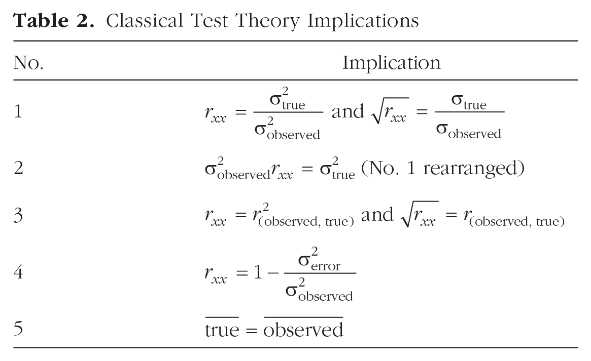
We note that among the implications presented in Table 2 is that there are various mathematically equivalent definitions of reliability (i.e., $r_{xx}$ ). Finally, we remind readers that classical test theory is a population-based theory and that the assumptions underlying it depend on there being a very large number of test takers (Lord & Novick, 1968). For example, one consequence of assuming a very large number of test takers is that true scores and random measurement errors can be considered uncorrelated. Another consequence is that when the standard deviation of errors (i.e., Standard Error of Measurement) is calculated, the resulting value is the standard deviation of a population of errors (not an estimate)—which is why a $z$ value is used in interval calculations rather than a $t$ value. ¹

Bivariate Regression: A Lens for Understanding Intervals

To properly understand what Standard Error of Estimation and Standard Error of Measurement are and their corresponding differences, it is crucial to understand bivariate linear regression. The reason for this is because both Standard Error of Estimation and Standard Error of Measurement are errors of prediction that arise from two different regression models (Gulliksen, 1950). Specifically, Standard Error of Estimation is the error in predicting true scores from observed scores, whereas Standard Error of Measurement is the error in predicting observed scores from true scores (Gulliksen, 1950). In the sections below, we explain these distinctions more comprehensively and thoroughly. Because Standard Error of Estimation and Standard Error of Measurement are errors that are derived from bivariate linear regression, we begin by reviewing a few key concepts from linear regression that are necessary to understand what the Standard Error of Estimation and Standard Error of Measurement are—and how they are different.

Model

When analyzing data, researchers often use a linear model, or a regression line, to describe the relation between two variables. In a measurement context, one can create a regression line that relates true scores to observed scores or vice versa. The slope of the regression line in this model is important because the regression line serves as the center point for a variety of measurement intervals.

In a two-variable regression, one variable serves as the criterion (i.e., the dependent variable), and one variable serves as the predictor. When graphing a regression, one places the criterion on the $y$ axis and the predictor on the $x$ axis (see Fig. 1a). In this type of graph, each dot represents a person. The regression line is a model of the linear relation between the predictor and the criterion.

Fig. 1.

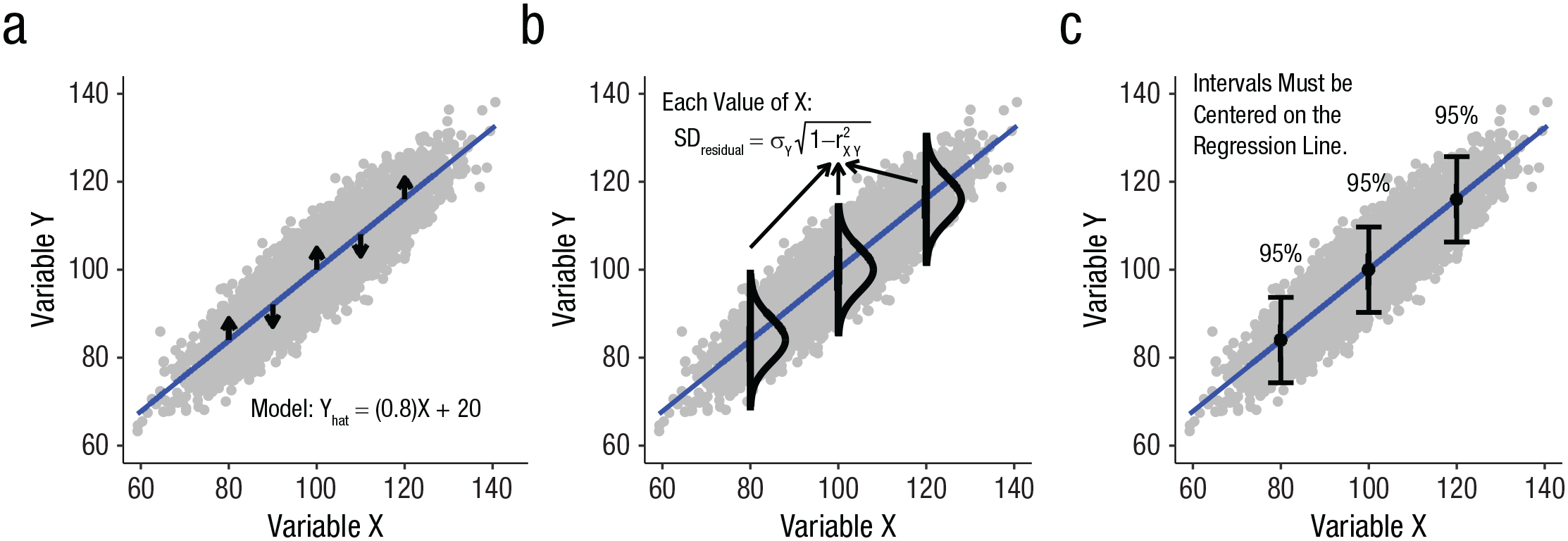
(a) Model. (b) Population for each x-axis value. (c) Capturing scores on y. Regression is the basis for many measurement models.

Describing the model: slope and intercept

In Figure 1a, we present a model in which the regression line has a slope of .80 and an intercept of 20. The slope refers to the angle of regression line, and the intercept refers to the elevation of the regression line (indicated by the position at which the line crosses the $y$ axis when $x=0$ ).

Slope is typically presented as the change in $y$ (i.e., $\Delta y$ ) divided by the change in $x$ (i.e., $\Delta x$ ). Consequently, when the slope is .80, this indicates that for every 1-unit change on the $x$ axis, the height of the regression line will increase by .80:

$$b=\frac{\Delta y}{\Delta x}=\frac{.80}{1}=.80.$$

There is, however, more than one way to describe the slope of a regression line. Indeed, when there is only one predictor, the correlation between $x$ and $y$ can be multiplied by the ratio of the standard deviations to also obtain the slope of the regression line. At different points, we use both approaches to conceptualizing slope:

$$b=r_{\left(X,Y\right)}\frac{{\sigma }_Y}{{\sigma }_X}=\left(0.8945529\right)\frac{10.00819}{11.18839}=.80.$$

Using the model: predicted values

The components of the regression model, slope and intercept, are typically presented in a regression equation like the one below:

$$\widehat{y}=.80x+20.$$

The regression equation is what one uses to generate the regression line. The regression line is effectively a series of predicted values. For a specified position on the $x$ axis, one can determine the $y$ value of corresponding spot above it on the regression line using the regression equation. This value is referred to as the $\widehat{y}$ value. All $\widehat{y}$ values (i.e., all predicted values) are on the regression line—in fact, they are what form the regression line.

A predicted value, a $\widehat{y}$ -value, can be obtained for any $x$ -axis value using the regression equation. For the position of 120 on the $x$ -axis, one can determine the corresponding $y$ -axis position of the regression line (i.e., the $\widehat{y}$ value) using the regression equation, which contains both the slope and the intercept:

$$\begin{array}{rr}\hfill \widehat{y}& \hfill =.80x+20\\ \hfill =.80\left(120\right)+20\\ \hfill =116\end{array}$$

Predicted values without an intercept

When working in a measurement context, one typically knows the slope of the regression line but unfortunately, not the intercept; this will become evident later. Consequently, we illustrate an alternative approach to calculating predicted scores (i.e., $\widehat{y}$ values) that can be used when the intercept is unknown. Obtaining a $\widehat{y}$ value when the intercept of the regression line is not known is possible as long as one knows the mean value on each axis (i.e., $\overline{x}$ and $\overline{y}$ ). These values are critical because a regression line will always run through the ( $\overline{x}$ , $\overline{y}$ ) point.

One can use the ( $\overline{x}$ , $\overline{y}$ ) point as a frame of reference to describe $\widehat{y}$ values on the regression line. An $x$ -axis position for the regression line is typically indicated by a specific value (e.g., $x=120$ ). However, one can also indicate that position as the distance from the mean value on the $x$ -axis. For example, if $\overline{x}=100$ , one could indicate the $x=120$ position as the difference from the mean, $120-100=20$ . Said another way, one can express any position on the $x$ -axis as a $\Delta x$ value from the mean of $x$ : $\Delta x=(x-\overline{x}$ ). Likewise, one can express any position on the $y$ -axis as a $\Delta y$ value from the mean of $y$ : $\Delta y=(y-\overline{y}$ ). We can combine this approach with typical formula for slope and some algebra to obtain an alternative formula for $\widehat{y}$ :

$$\begin{array}{rr}\hfill b& \hfill =\frac{\Delta y}{\Delta x}\\ \hfill b\left(\Delta x\right)& \hfill =\Delta y\\ \hfill \Delta y& \hfill =b\left(\Delta x\right)\\ \hfill \left(\widehat{y}-\overline{y}\right)& \hfill =b\left(x-\overline{x}\right)\\ \hfill \widehat{y}& \hfill =\overline{y}+b\left(x-\overline{x}\right)\end{array}$$

Moving forward, we refer to Equation 2 as the “no-intercept approach” to predicted values:

$$\widehat{y}=\overline{y}+b\left(x-\overline{x}\right).$$

(2)

Revisiting the previously described scenario in which we are interested in obtaining a $\widehat{y}$ value for $x=120$ . The slope is .80 and $\overline{x}=100$ :

$$\begin{array}{rr}\hfill \widehat{y}& \hfill =\overline{y}+b\left(x-\overline{x}\right)\\ \hfill =100+.8\left(120-100\right)\\ \hfill =116\end{array}$$

We can see the $\widehat{y}$ value we obtain is 116—the same as the value we obtained using the regression equation. Understanding the no-intercept approach to predicted values is crucial for understanding both Standard Error of Estimation and Standard Error of Measurement as the regression models underlying these errors do not have known intercepts.

Interpretation of predicted values

The proper interpretation of predicted values (i.e., $\widehat{y}$ values) is critical to properly interpreting the Standard Error of Estimation and, unfortunately, is not intuitive. Because of this, we devote a little time to go over the proper interpretation of predicted values. Consider the scenario from the previous section. We might imagine that Adriana has a score of 120 on the $x$ -axis and that we want to obtain a predicted score for Adriana. Using either of the prediction approaches, we obtain a $\widehat{y}$ value of 116. Unfortunately, many people tend to think of the predicted value of 116 as being specific to Adriana—it is not.

To properly interpret the $\widehat{y}=116$ , we need to remember that Adriana is not the only one with an $x$ -axis score of 120 in the regression model. There are many participants with an $x$ -axis score of 120. In fact, we can imagine that there is an entire population of $y$ values (all different) for everyone with an $x$ -axis score of 120. Indeed, there is a population of $y$ values for each value on the $x$ -axis, as illustrated in Figure 1b.

Because there is an entire population of $y$ values at the $x$ -axis value of 120, the predicted value of 116 is not an individualized prediction. Instead, 116 is a predicted $y$ -axis score for everyone with an $x$ -axis value of 120. More specifically, $\widehat{y}=116$ is an estimate of the population mean, on the $y$ -axis, for everyone with an $x$ -axis value of 120. Understanding this point is crucial for understanding measurement intervals.

Errors

The vertical distance between each point (representing a person) in the scatter plot and the regression line is called a “residual.” Of particular interest in a regression is how close the points are to the regression line. The overall vertical closeness of all the points to the regression line is indexed by the variance of the residuals. The typical formula for the variance of residuals is presented in Equation 3:

$${\sigma }_{residual}^2=\frac{{\displaystyle \sum }{\left(y_i-\widehat{y_i}\right)}^2}{n-2}.$$

(3)

In the measurement context, however, we use an alternative formula for the variance of residuals (see Allen, 1997). This alternative formula, which provides the same result when $N$ is large, as it is in classical test theory, is presented in Equation 4 below:

$${\sigma }_{residual}^2={\sigma }_y^2\left(1-r_{xy}^2\right).$$

(4)

Taking the square root, we obtain the formula for the standard deviation of residuals in Equation (5) below:

$${\sigma }_{residual}={\sigma }_y\sqrt{1-r_{xy}^2}.$$

(5)

Homogeneity of residuals

In linear regression, there are several assumptions. One assumption that is relevant for the calculation of measurement intervals is homoscedasticity. Homoscedasticity means that the variance of the residuals around a regression line is the same for all values on the $x$ -axis (Cohen et al., 2003). We previously imagined that there is a population of $y$ -axis values for each position along the $x$ -axis (see Figure 1b). If we consider only those people with an $x$ -axis score of 120, the variance of the residuals for these people is the same as the overall variance of the residuals obtained by using Equation 5. This homoscedasticity assumption applies to all values along the $x$ -axis and is important for the calculation of measurement intervals. With measurement intervals, we calculate quantities based on an entire data set and then apply them to a thin slice of the data set that is relevant to a particular $x$ -axis value to establish the length of the interval (see Figure 1c). The homoscedasticity assumption underlies the logic of this approach.

Summary

Because Standard Error of Measurement and Standard Error of Estimation are derived from different bivariate linear regression models, the regression principles outlined above will make it possible to more clearly understand what Standard Error of Estimation and Standard Error of Measurement intervals are and how they are different.

SEE Many-Test-Takers Model

The Standard Error of Estimation interval provides a way to understand the variability in true-score scores for the many test takers that share a specified observed score. The Standard Error of Estimation interval has sometimes been presented as a preferred interval to construct around test scores (Dudek, 1979). This preference for the Standard Error of Estimation interval is predicated on the misunderstanding that the Standard Error of Measurement interval is not useful for predicting true scores (e.g., Charter & Feldt, 2001; Dudek, 1979; Harvill, 1991). We believe that the misinterpretation of Standard Error of Measurement interval is often rooted in a misunderstanding of the Standard Error of Estimation interval. Consequently, we present an explanation of the Standard Error of Estimation interval and its associated regression model before presenting the Standard Error of Measurement interval.

Standard Error of Estimation is the error made in trying to predict true scores from observed scores (Gulliksen, 1950). Gulliksen (1950) emphasized this orientation when he called it the error in estimating true score. He specifically stated that it is “the error made in using the best fitting regression equation to predict the true score from observed score” (p. 43). Consequently, to understand Standard Error of Estimation, it needs to be viewed in the context of a regression model in which observed scores predict true scores.

Correspondingly, we present in Figure 2 a regression model for the Standard Error of Estimation. In Figure 2, observed scores are represented on the $x$ -axis, and true scores are represented on the $y$ -axis. Recall from classical test theory that an observed score is defined as the sum of a true score and random measurement error (Equation 1). The regression model in Figure 2 is created by plotting two of these three components (i.e., observed scores and true scores) for a large number of people (i.e., a population).

Fig. 2.

Standard Error of Estimation Many-Test-Taker regression model.

Note that in an applied measurement context, one does not know true scores. As a result, it is not possible, in an applied context, to construct a measurement regression model like the one in Figure 2. Nonetheless, this conceptual regression model provides the theoretical basis for the Standard Error of Estimation interval.

Model slope

The slope of the regression line in this model is important because it influences the point around which the Standard Error of Estimation interval is centered. In the Standard Error of Estimation regression model presented in Figure 2, the slope of the regression line is equal to the reliability ( $r_{xx}$ ). This is a characteristic that occurs with the Standard Error of Estimation regression model but not the Standard Error of Measurement regression model. To illustrate why this is so, we present an algebraic derivation drawing from classical test theory.

To begin, we represent slope as the correlation between X and Y multiplied by the ratio of the standard deviations for Y and X:

$$b=r_{\left(X,Y\right)}\frac{{\sigma }_Y}{{\sigma }_X}.$$

Next, we replace X with “observed scores” and Y with “true scores” because this corresponds with the Standard Error of Estimation regression model in which observed scores are on the $x$ -axis and true scores are on the $y$ -axis (Fig. 2):

$$\begin{array}{rr}\hfill b& \hfill =r_{\left(X,Y\right)}\frac{{\sigma }_Y}{{\sigma }_X}\\ \hfill =r_{\left(observed,true\right)}\frac{{\sigma }_{true}}{{\sigma }_{observed}}& \hfill .\end{array}$$

Then, drawing from classical test theory, we substitute the correlation between observed scores and true scores with the square root of reliability, $\sqrt{r_{xx}}=r_{\left(\mathrm{observed},\mathrm{true}\right)}$ (see Classical Test Theory Implication 3 in Table 1):

$$\begin{array}{rr}\hfill b& \hfill =r_{\left(observed,true\right)}\frac{{\sigma }_{true}}{{\sigma }_{observed}}\\ \hfill =\sqrt{r_{xx}}\frac{{\sigma }_{true}}{{\sigma }_{observed}},ClassicalTestTheoryImplication3:\sqrt{r_{xx}}=r_{(true,observed)}& \hfill .\end{array}$$

Next, based on the definition of reliability in classical test theory (see classical Test Theory Implication 1 in Table 1), where $\sqrt{r_{xx}}=\frac{{\sigma }_{true}}{{\sigma }_{observed}}$ , we make a substitution. Following this substitution, we can perform a few simplifying mathematical operations to arrive at $r_{xx}$ :

$$\begin{array}{rr}\hfill b& \hfill =\sqrt{r_{xx}}\frac{{\sigma }_{true}}{{\sigma }_{observed}}\\ \hfill =\frac{{\sigma }_{true}}{{\sigma }_{observed}}\frac{{\sigma }_{true}}{{\sigma }_{observed}},ClassicalTestTheoryImplication1:\sqrt{r_{xx}}=\frac{{\sigma }_{true}}{{\sigma }_{observed}}\\ \hfill =\frac{{\sigma }_{true}^2}{{\sigma }_{observed}^2}\\ \hfill =r_{xx}\end{array}.$$

Thus, we can see that in Standard Error of Estimation Model, where observed scores predict true scores, the slope of the regression line is equal to the reliability ( $r_{xx}$ ) by definition. In Figure 2, the reliability of the data is .80, so the slope of the regression line/model is $b=0.80$ .

Interval center

For the Standard Error of Estimation interval to perform properly, it must be centered on the regression line. That is, for a given observed score (i.e., $x$ -axis value), the resulting interval must the centered on the $\widehat{y}$ value associated with that observed score in the Standard Error of Estimation regression model. If the slope of the regression line were 1.00, this would be a trivial task because it would mean that $\widehat{y}=x$ (i.e., $\widehat{true}=observed$ ). However, when the slope is not 1.00, then $\widehat{y}\ne x$ ≠ x, and this simple rule will not suffice.

In the Standard Error of Estimation regression model, where the slope of the regression line is the reliability ( $b=r_{xx}$ ), we can obtain a $\widehat{y}$ value using the no-intercept-prediction approach discussed in the section, Bivariate Regression: A Lens for Understanding Intervals. Specifically, Equation 2 can be used to find $\widehat{y}$ for a specific $x$ -axis value when all we know is the slope ( $b=r_{xx}$ ) and the mean value for each axis (i.e., $\overline{x},\overline{y}$ ):

$$\widehat{y}=\overline{y}+b\left(x-\overline{x}\right).$$

In the context of the Standard Error of Estimation, we can replace $y$ values with “true” scores and $x$ values with “observed” scores because true scores are being predicted by observed scores. In addition, we know the slope ( $b$ ) is equal to the reliability ( $r_{xx}$ ) in the Standard Error of Estimation Model. Consequently, once we substitute these terms into Equation 2, we have the equation below:

$$\begin{array}{rrr}\hfill {\widehat{y}}_{true}& \hfill =\overline{true}+r_{xx}\left(\mathrm{observed}-\overline{\mathrm{observed}}\right)& \hfill .\end{array}$$

Unfortunately, this new equation is still problematic for practical purposes. Although we have an equation that will allow us to generate a prediction of ${\widehat{y}}_{true}$ , this equation requires us to know the mean value of all participants true scores (i.e., $\overline{true}$ ). Because true scores are unknown, we can never know $\overline{true}$ . Fortunately, we know that because measurement errors are considered random, the mean of the random measurement errors is zero. Correspondingly, because observed scores are the sum of true score and random measurement errors, the mean observed score will equal the mean true score (because the mean measurement error is zero). Said the other way around, the mean of true scores ( $\overline{true}$ ) is equal to the mean of observed scores ( $\overline{observed}$ ); see Classical Test Theory Implication 5 in Table 1. The implication of this is that we can perform the substitution illustrated below:

$$\begin{array}{rr}\hfill {\widehat{y}}_{true}& \hfill =\overline{true}+r_{xx}\left(\mathrm{observed}-\overline{\mathrm{observed}}\right)\\ \hfill =\overline{observed}+r_{xx}\left(o\mathrm{bserved}-\overline{\mathrm{observed}}\right)& \hfill .\end{array}$$

Thus, we obtain a practical formula for the predicted true score value: ${\widehat{y}}_{true}$ , presented in Equation 6:

$${\widehat{y}}_{\mathrm{true}}=\overline{\mathrm{observed}}+r_{xx}\left(\mathrm{observed}-\overline{\mathrm{observed}}\right).$$

(6)

Equation 6 is a way of determining the spot on the regression line, ${\widehat{y}}_{true}$ , associated with a specified observed score (i.e., $x$ -axis value). This ${\widehat{y}}_{true}$ value is used as the center for the Standard Error of Estimation interval.

Note that ${\widehat{y}}_{true}$ is an estimate of the mean of the true scores for all individuals with a particular observed score. It is not the true score for a specific individual based on a single observed score. This is a critical point to establish to be able to correctly interpret the Standard Error of Estimation interval. To put more emphasis on this point, because of the regression model on which it is based, the Standard Error of Estimation is necessarily interpreted with respect to the true scores of many people. This means that any given interval constructed with the Standard Error of Estimation does not refer to the capture of a single individual’s true score; it does refer to capturing the true scores of many test takers with the same observed score.

Interval length: Standard Error of Estimation as the standard deviation of residuals

The Standard Error of Estimation regression line defines the relation between observed scores on the $x$ -axis and true scores on the $y$ -axis. This line will be the center for the Standard Error of Estimation interval for any given observed score (i.e., point on the $x$ -axis). However, to create an interval around the regression line at a specific point, we need to know how long to make the interval. That is, we need to know the extent to which true scores vary around the regression line—and use this as the basis for setting the length of the interval. In other words, we want to know the standard deviation of residuals for the Standard Error of Estimation Model; see Equation 7. This value is commonly referred to as the Standard Error of Estimation error term:

$${\sigma }_{residual-SEE}={\sigma }_{observed}\sqrt{\left(1-r_{xx}\right)\left(r_{xx}\right)}.$$

(7)

An understanding of why the ${\sigma }_{residual-SEE}$ equation takes this form can be obtained by rearranging Equation 4 from our Bivariate Regression: A Lens for Understanding section. Equation 4 provides the variance of residuals for a bivariate regression model, repeated below:

$$\begin{array}{rrr}\hfill {\sigma }_{\mathrm{residual}}^2& \hfill ={\sigma }_y^2\left(1-r_{xy}^2\right)& \hfill .\end{array}$$

We adapt Equation 4 to the Standard Error of Estimation Model by relabeling the X and Y variables as previously described. In Figure 2, we have true scores along the $y$ -axis. Consequently, we replace Y in Equation 4 with “true.” This results in ${\sigma }_y^2$ becoming ${\sigma }_{true}^2$ . Correspondingly, because we have observed scores on the $x$ -axis, we replace X in Equation 4 with “observed.” This second change results in the squared correlation between X and Y ( $r_{xy}^2$ ) becoming the squared correlation between true scores and observed scores ( $r_{(true,observed)}^2$ ). We make these substitutions below:

$$\begin{array}{rr}\hfill {\sigma }_{\mathrm{residual}-\mathrm{SEE}}^2& \hfill ={\sigma }_y^2\left(1-r_{xy}^2\right)\\ \hfill ={\sigma }_{true}^2\left(1-r_{(true,observed)}^2\right).\end{array}$$

Furthermore, we know that the squared correlation between true and observed scores, $r_{(true,observed)}^2$ , is also equal to the reliability, $r_{xx}$ (see Classical Test Theory Implication 3 in Table 1). Thus, we can make the following substitution:

$$\begin{array}{rr}\hfill {\sigma }_{\mathrm{residual}-\mathrm{SEE}}^2& \hfill ={\sigma }_{true}^2\left(1-r_{(true,observed)}^2\right)\\ \hfill ={\sigma }_{true}^2\left(1-r_{xx}\right)\end{array}.$$

In addition, we also know that the variance of true scores, ${\sigma }_{true}^2$ , is equal to the variance of observed scores multiplied by the reliability, ${\sigma }_{observed}^2{r}_{xx}$ (see Classical Test Theory Implication 2 in Table 1). This allows us to make the following substitution:

$$\begin{array}{rr}\hfill {\sigma }_{\mathrm{residual}-\mathrm{SEE}}^2& \hfill ={\sigma }_{true}^2\left(1-r_{xx}\right)\\ \hfill ={\sigma }_{observed}^2{r}_{xx}\left(1-r_{xx}\right)\\ \hfill ={\sigma }_{observed}^2\left(1-r_{xx}\right)r_{xx}& \hfill .\end{array}$$

Taking the square root results in the following:

$${\sigma }_{residual-SEE}={\sigma }_{observed}\sqrt{\left(1-r_{xx}\right)r_{xx}}.$$

This is the formula for the Standard Error of Estimation error term. Thus, the formula for the ${\sigma }_{residual-SEE}$ term follows directly from Equation 5 describing the standard deviation of residuals in a bivariate regression model. Consequently, it is evident that the Standard Error of Estimation formula is the standard deviation of residuals in a bivariate regression model where true scores are predicted by observed scores.

Interpreting s_{residual–SEE} ${\sigma }_{residual-SEE}$ through the lens of homoscedasticity

With the above illustration, we can see how ${\sigma }_{residual-SEE}$ is the standard deviation of the true scores around the regression line when observed scores predict true scores (Fig. 2). Note that there are two correct interpretations of the ${\sigma }_{residual-SEE}$ . First, we can consider ${\sigma }_{residual-SEE}$ to be the standard deviation of true scores around the regression line based on the scores of all individuals (see Fig. 2). This conceptual interpretation is consistent with the calculation method because the residuals for all test takers are used in the calculation.

Second, because of the homoscedasticity assumption, we can consider ${\sigma }_{residual-SEE}$ as referring to the standard deviation of true scores around the regression at a specific observed score on the $x$ -axis. Applying the homoscedasticity assumption (see Fig. 1b) allows us to state that ${\sigma }_{residual-SEE}$ is also the standard deviation of true scores for those individuals with a specific observed score (e.g., 90; see Fig. 2) even though ${\sigma }_{residual-SEE}$ was calculated using information from all individuals. This second interpretation of ${\sigma }_{residual-SEE}$ is consistent with Dudek’s (1979) description of the Standard Error of Estimation error term as the “standard deviation of true scores if the observed score is held constant” (p. 336).

Interval construction and interpretation

A Standard Error of Estimation interval can be constructed using Equation 8 below, which uses the previously described predicted true score value, ${\widehat{y}}_{true}$ , and the standard deviation of residuals, ${\sigma }_{residual-SEE}$ :

$$SEEMany-Test-TakersInterval={\widehat{y}}_{true}\pm z\times {\sigma }_{residual-SEE}.$$

(8)

Typically, the Standard Error of Estimation interval calculation begins with a single observed score for a specific individual. However, it is important to recognize that the Standard Error of Estimation interval does not provide information about that single person’s true score. The Standard Error of Estimation intervals provide information about the true scores for all individuals with that particular observed score.

Consider, for example, that we collected data from a large number of people, and the reliability of observed scores is .80 ( $r_{xx}=.80$ ) with a mean of 100 ( $M$ = 100) and a standard deviation of 10 ( $SD$ = 10). We want to construct a Standard Error of Estimation interval based on the observed score of a single person named Dromio. We know Dromio’s observed score is 90. So, we calculate an estimated mean true score for all individuals with an observed score of 90. To do so, we need to know the slope of the regression line. We know the slope of the regression line is $b=0.80$ because in a Standard Error of Estimation Model, $b=r_{xx}$ :

$$\begin{array}{rr}\hfill {\widehat{y}}_{\mathrm{true}}& \hfill =\overline{\mathrm{observed}}+{\mathrm{r}}_{xx}\left(\mathrm{observed}-\overline{\mathrm{observed}}\right)\\ \hfill =100+.80\left(90-100\right)\\ \hfill =92& \hfill .\end{array}$$

This calculation indicates that our estimate of the mean true score for those individuals with an observed score of 90 is 92 (i.e., ${\widehat{y}}_{true}=92$ ). We use this as the center of the interval. Next, we want to calculate for those individuals with an observed score of 90 the standard deviation of true scores:

$$\begin{array}{rr}\hfill {\sigma }_{residual-SEE}& \hfill ={\sigma }_{observed}\sqrt{\left(1-r_{xx}\right)\left(r_{xx}\right)}\\ \hfill =\left(10\right)\sqrt{\left(1-.80\right)\left(.80\right)}\\ \hfill =4.0& \hfill .\end{array}$$

This second calculation indicates that for those individuals with an observed score of 90, the standard deviation of true scores is 4.0 (i.e., ${\sigma }_{residual-SEE}=4.0$ ). We can now construct the Standard Error of Estimation interval:

$$\begin{array}{rr}\hfill 95\mathrm{\%}SEEMany-Test-TakersInterval& \hfill ={\widehat{y}}_{true}\pm z\times {\sigma }_{residual-SEE}\\ \hfill =92\pm 1.96\times 4.0\\ \hfill =[84.16,99.84]& \hfill .\end{array}$$

Thus, based on an observed score of 90, we obtain 95% Standard Error of Estimation = [84.16, 99.84]. How do we interpret this SEE Many-Test-Takers Interval? In Figure 2, there is more than one person with an observed score of 90. Moreover, people with an observed score of 90 do not all have the same true score. Indeed, for people with an observed score of 90, there is a wide range of true scores that are possible. Thus, the 95% SEE is a range that bounds the middle 95% of true scores for people with a particular observed score. In other words, this interval indicates that for the many individuals with an observed score of 90, 95% of them have true scores between 84.16 and 99.84. Recall that this interval was created using the logic of classical test theory—which is a population-level theory (Lord & Novick, 1968). As result, we need to remember that we are considering the scores presented in Figure 2 as a population. Because of the population assumption of classical test theory, the SEE Many-Test-Takers Interval is effectively a parameter describing a range of the data at a particular point—inference is not involved. Because inference is not involved, this interval is not a confidence interval—just a range. We note that if we considered our data a sample, the resulting interval would be a prediction interval (see Cumming & Calin-Jageman, 2016); however, the population assumption of classical test theory facilitates interpreting it in the way we have described (see Appendix A1).

Standard Error of Measurement

Perhaps the most popular error term that is used to construct intervals around test scores is the Standard Error of Measurement. This error term is regularly covered in psychological-measurement textbooks and psychometric education. Despite the widespread use and teaching of Standard Error of Measurement, intervals based on this error have been subject to a multitude of interpretations. These varying interpretations have led to disagreements in the testing literature with respect to what is a correct interpretation and what is a misinterpretation (Charter & Feldt, 2001; Dudek, 1979; Harvill, 1991; Nunnally & Bernstein, 1994). One potential cause of confusion surrounding Standard Error of Measurement may be that it can be correctly interpreted several different ways. Indeed, Gulliksen (1950) devoted an entire chapter to the topic, appropriately titled “Various Interpretations of the Error of Measurement”; “error of measurement” is the term Gulliksen used for Standard Error of Measurement.

To help understand Standard Error of Measurement, in this section, we focus primarily on two common approaches to conceptualizing it. The first approach considers a scenario in which there are many test takers and the Standard Error of Measurement is the error term in a bivariate regression. The second approach considers a scenario in which there is a single individual and the Standard Error of Measurement is the error term for a population of observed scores for that individual. We begin with the many-test-takers scenario.

SEM Many-Test-Takers model

One approach to conceptualizing Standard Error of Measurement relies on a scenario in which there are many test takers. In this scenario, the true scores are used to predict observed scores via a bivariate regression model. We illustrate this model in Figure 3. This model is an inversion of the model we reviewed for Standard Error of the Estimate, in which observed scores predicted true scores. Consistent with Figure 3, Standard Error of Measurement is the standard error when predicting observed scores using true scores (Gulliksen, 1950; Nunnally & Bernstein, 1994). More practically, the Standard Error of Measurement regression interval can be thought of as a way to understand the variability in observed scores for the many test takers that share a specific true score.

Fig. 3.

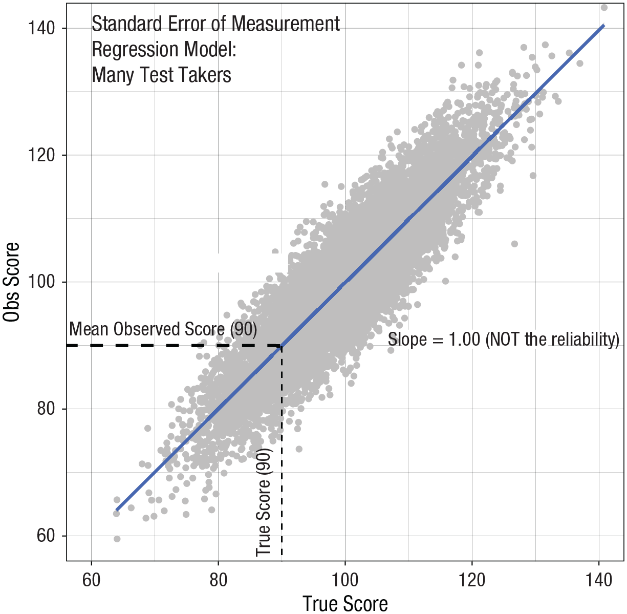
Standard Error of the Measurement Many-Test-Taker regression model.

Model slope

The slope of the regression line in the Standard Error of Measurement regression is 1.00. This deviates with the Standard Error of Estimation scenario in which the slope was equal to the reliability. To understand why the slope is 1.0 in a Standard Error of Measurement Model, we begin by representing slope as the correlation between X and Y multiplied by the ratio of the standard deviations for X and Y:

$$b=r_{\left(X,Y\right)}\frac{{\sigma }_Y}{{\sigma }_X}.$$

Following this, we replace X with “true scores” and replace Y with “observed scores” because this corresponds with the Standard Error of Measurement regression model in which observed scores are on the $x$ -axis and true scores are on the $y$ -axis (Fig. 3):

$$b=r_{\left(true,observed\right)}\frac{{\sigma }_{\mathrm{observed}}}{{\sigma }_{\mathrm{true}}}$$

Drawing from classical test theory, we can substitute the correlation between true scores and observed scores with the square root of reliability $r_{\left(\mathrm{true},\mathrm{observed}\right)}=\sqrt{r_{xx}}$ (see classical Test Theory Implication 3 in Table 1):

$$\begin{array}{rr}\hfill b& \hfill =r_{\left(true,observed\right)}\frac{{\sigma }_{\mathrm{observed}}}{{\sigma }_{\mathrm{true}}}\\ \hfill =\sqrt{r_{xx}}\frac{{\sigma }_{\mathrm{observed}}}{{\sigma }_{\mathrm{true}}},ClassicalTestTheoryImplication3:\sqrt{r_{xx}}=r_{(true,observed)}.\end{array}$$

However, Classical Test Theory Implication 1 indicates that the square root of the reliability is equal to the ratio of the true-score standard deviation divided by the observed-score standard deviation:

$$\begin{array}{rr}\hfill b& \hfill =\sqrt{r_{xx}}\frac{{\sigma }_{\mathrm{observed}}}{{\sigma }_{\mathrm{true}}}\\ \hfill =\frac{{\sigma }_{\mathrm{true}}}{{\sigma }_{\mathrm{observed}}}\frac{{\sigma }_{\mathrm{observed}}}{{\sigma }_{\mathrm{true}}},ClassicalTestTheoryImplication1:\frac{{\sigma }_{true}}{{\sigma }_{observed}}=\sqrt{r_{xx}}& \hfill .\end{array}$$

Next, some simple rearranging of terms illustrates that the slope is equal to 1.00:

$$\begin{array}{rr}\hfill b& \hfill =\frac{{\sigma }_{\mathrm{true}}}{{\sigma }_{\mathrm{observed}}}\frac{{\sigma }_{\mathrm{observed}}}{{\sigma }_{\mathrm{true}}}\\ \hfill =\frac{{\sigma }_{\mathrm{true}}}{{\sigma }_{\mathrm{true}}}\frac{{\sigma }_{\mathrm{observed}}}{{\sigma }_{\mathrm{observed}}}\\ \hfill =\left(1.00\right)\left(1.00\right)\\ \hfill =1.00& \hfill .\end{array}$$

Thus, we can see that in the regression model, on which the Standard Error of Measurement is based, must have a slope of 1.00. Understanding the slope is 1.00 is critical to determining how to center the interval on the regression line.

Interval center

In the Standard Error of Measurement regression model, if we want to create an interval, we do so at a specific true score along the $x$ -axis. Recall that each value along the $x$ -axis can be used indicate a vertical population of $y$ -axis values (i.e., observed-score values). An inspection of Figure 3 illustrates that for each true-score value on the $x$ -axis, there are many test takers, each with a different observed score. Consequently, each ${\widehat{y}}_{\mathrm{observed}}$ value on the regression line is the estimated mean of a population of observed scores for test takers that share the same true score on the $x$ -axis. Recall that the slope for this regression model is 1.00. This means that for all test takers with a true score of 85, the estimated mean observed score for this group is also 85. This is consistent with classical test theory in which errors are defined as being random and thus are expected to have a mean of zero.

Interval length

The length of a vertical interval around the regression line, at a specific true-score value on the $x$ -axis, depends on the dispersion of the points around the regression line. This dispersion is indexed by the standard deviation of the residuals (see Equation 9). For the regression model illustrated in Figure 3, the standard deviation of residuals is called the Standard Error of Measurement (Nunnally & Bernstein, 1994):

$${\sigma }_{residual-SEM}={\sigma }_{observed}\sqrt{\left(1-r_{xx}\right)}.$$

(9)

To further understand this definition, we start with Equation 4 for the variance of residuals in a regression line (see Allen, 1997). Then, we replace X and Y with “true scores” and “observed scores,” respectively:

$$\begin{array}{rr}\hfill {\sigma }_{residual-SEM}& \hfill ={\sigma }_y^2\left(1-r_{xy}^2\right)\\ \hfill ={\sigma }_{\mathrm{observed}}^2\left(1-r_{xx}\right)& \hfill .\end{array}$$

We then take the square root to obtain the final equation below. We note that this equation can also be obtained by rearranging the classical test theory reliability formula—as illustrated in Appendix A2:

$${\sigma }_{residual-SEM}={\sigma }_{observed}\sqrt{\left(1-r_{xx}\right)}.$$

Thus, we can see that the Standard Error of Measurement is linked to a regression model in which observed scores are predicted by true scores and is specifically the standard deviation of errors around the regression line of this model. This is consistent with Gulliksen (1950), who stated, “The error of estimate derived from the regression of observed upon true scores is the same as the error of measurement” (p. 49).

Because the Standard Error of Measurement is embedded in a regression model, we can also understand how the assumption of homoscedasticity applies here as well. Homoscedasticity means that the standard deviation of observed scores on the $y$ -axis will be the same for all true-score values on the $x$ -axis. Practically, this means that the same Standard Error of Measurement is used to construct an interval around the regression line for all true-score values on the $x$ -axis.

Interval construction and interpretation

To construct an interval with Standard Error of Measurement, Equation 10 below, which uses the previously described predicted true-score value, ${\widehat{y}}_{\mathrm{observed}}$ , and the standard deviation of residuals, ${\sigma }_{residual-SEM}$ , can be used:

$$95\mathrm{\%}SEMMany-Test-TakersInterval=true\pm z\times {\sigma }_{residual-SEM}.$$

(10)

The Standard Error of Measurement regression interval differs in several ways from the Standard Error of Estimation regression interval. Perhaps most important, the Standard Error of Estimation regression interval is arguably a practical interval for individuals interested in interpreting a test score. Although the Standard Error of Estimation regression interval is not specific to a single individual, it can provide useful contextual information for a person with a particular observed score. For example, if an individual received an observed score of 90 on a test, users of a Standard Error of Estimation regression interval could tell the individual that although they do not know the individual’s true score on this test, they do know that 95% of people with this observed score have a true score between 100.16 and 115.84. In contrast, the Standard Error of Measurement regression interval uses a true score as the starting point for the calculation of the interval. Consequently, it does not provide a useful approach for interpreting observed test scores.

The Standard Error of Measurement regression interval is useful, however, for asking theoretical “What if?” questions. An example of a theoretical “What if?” question could be the following: “Imagine we have a very large number of people take a test and we obtain a reliability of .80 and the standard deviation of observed scores is 10. For those test takers with a true score of 90, what is the range of observed scores that could be expected?” To answer a theoretical question of this sort, we construct a 95% Standard Error of Measurement regression interval in the following way:

$$\begin{array}{rr}\hfill 95\mathrm{\%}SEMMany-Test-TakersInterval& \hfill =true\pm z\times {\sigma }_{residual-SEM}\\ \hfill =90\pm 1.96\times 10\sqrt{1-.80}\\ \hfill =90\pm 8.765386\\ \hfill =[81.2,98.8]& \hfill .\end{array}$$

This results in a 95% SEM-Regression = [81.2, 98.8] for a true score of 90. This interval indicates that of the many individuals with a true score of 90, 95% of them recorded observed scores between 81.2 and 98.8. To aid with the interpretation, it may help to consult Figure 3. Here, we can see that there is more than one person with a true score of 90 and that of the people with a true score of 90, not all of them have the same observed score. Indeed, for people with a true score of 90, there is a wide range of observed scores. The 95% Standard Error of Measurement interval is a range that bounds the middle 95% of observed scores values for people with a particular true score. Again, although this is theoretically interesting, it does not aid in the interpretation of a test taker’s score. As discussed previously, because classical test theory is a population-level theory, this SEM Many-Test-Takers Interval is a range, not a confidence interval; see the SEE Many-Test-Takers Interval section for a full discussion.

Recall this interval was created using the logic of classical test theory—which is a population-level theory (Lord & Novick, 1968). As a result, we need to remember that we are considering the scores presented in Figure 3 as a population. Because of the population assumption of classical test theory, the SEM Many-Test-Takers Interval is effectively a parameter describing a range of the data at a particular point—inference is not involved. Because inference is not involved, this interval is not a confidence interval—it is simply a range. We emphasize that if we considered our data to be a sample, the resulting would be a prediction interval (see Cumming & Calin-Jageman, 2016); however, the population assumption of classical test theory facilitates interpreting it in the way we have described (see Appendix A1).

SEM Single-Test-Taker model

From a practical standpoint, the most critical question for any test taker is the following: Given my observed score, what is my likely true score? Fortunately, it is possible to use the Standard Error of Measurement to create an interval that provides the test taker with this information. Accomplishing this objective requires us to view Standard Error of Measurement through a different lens—one that deviates from the regression-based model. The calculation of the Standard Error of Measurement stays the same in this context. ²

This new lens requires that we imagine a scenario in which there is a single person that takes a test a very large number of times. In this imaginary scenario, each time the person takes a test, the person has no memory of previous attempts and are not influenced by those previous attempts. The result is a large number (i.e., a population) of observed scores for a test taker—a distribution of observed scores (see Figure 4). The true score for this test taker is conceptualized as a population mean ( $\mu$ ), and the observed scores are the elements of the population. Conceptualizing the true score as the mean of the population should be familiar to people acquainted with classical test theory because it is the definition of true score (Lord & Novick, 1968). In this view, a large number of independent observed scores for a single test taker ( $O$ ) differ from the true score because of random measurement error. The standard deviation of these observed scores for a single test taker is the Standard Error of Measurement, which is represented by the term ${\sigma }_{error}$ . This interpretation is consistent with the interpretation of Standard Error of Measurement as the standard deviation of observed scores over a large number of randomly parallel tests (Nunnally & Bernstein, 1994).

Fig. 4.

Standard Error of the Measurement Single-Test-Taker model.

Interval construction and interpretation

This population model of observed scores for an individual allows us to use Standard Error of Measurement to construct an interval around a specific observed score for a test taker that will capture the test taker’s true score with a specified probability. The logic of using an interval to capture a test taker’s true score from an observed score is the same as that used in inferential statistics to capture a population mean based on a sample mean. Consequently, the Standard Error of Measurement interval in this model is a confidence interval. Confidence intervals are, however, prone to misinterpretation (see Hoekstra et al., 2014; Thompson, 2007).

As outlined above, a Standard-Error-of-Measurement-based confidence interval can be constructed using Equation 11:

$$SEMSingle-Test-TakerInterval=observed\pm z\times {\sigma }_{error}.$$

(11)

To understand how to interpret this interval, we can consider an example. Imagine that we collected data from a large number of people and that for the observed scores, we know the reliability ( $r_{xx}=.80$ ) and descriptive statistics ( $M=100$ and $SD=10$ ). We want to construct a Standard Error of Measurement interval based on the observed score of a single person named Emilia. We know Emilia’s observed score is 90:

$$\begin{array}{rr}\hfill 95\mathrm{\%}SEMSingle-Test-TakerInterval& \hfill =observed\pm z\times {\sigma }_{error}\\ \hfill =observed\pm z\times {\sigma }_{observed}\sqrt{\left(1-r_{xx}\right)}\\ \hfill =90\pm 1.96\times 10\sqrt{\left(1-.80\right)}\\ \hfill =90\pm 8.765386\\ \hfill =[81.23461,98.765386]& \hfill .\end{array}$$

Thus, based on Emilia’s observed score of 90, we obtain the 95% SEM = [81.23, 98.76]. How do we interpret this interval? The first step is to recognize that this is a confidence interval. Before Emilia takes the test, we can say there is a 95% chance the interval we obtain after the test will contain her true score. After data collection (i.e., test administration), once we have a specific interval with end points, we can only state that we have an interval estimate of the true score—the 95% probability should not be invoked to interpret the specific end points of this interval (Thompson, 2007). To correctly interpret this interval, it is important to realize that the SEM Single-Test-Taker Interval is a confidence interval. It is a confidence interval because we are trying to estimate a population mean using a sample mean. We consider the set of all possible observed scores for Emilia as a population. Emilia’s single observed score (90) is a sample mean ( $n$ = 1). We are merely creating an interval around our sample mean to estimate the population mean (i.e., Emilia’s true score). Recall from Table 2 that the mean of all possible observed scores (i.e., the mean of the population of observed scores) is the true score for an individual.

Myths: Standard Error of Measurement

Unfortunately, many attempts to clarify and provide direction with respect to the proper interpretation of Standard Error of Measurement have only served to add confusion. One reason for this is that some clarification attempts essentially “mix and match” from the models described above, providing an interpretation that is not consistent with any correct interpretation. In other cases, the interpretation error is idiosyncratic and is simply an incorrect confidence-interval interpretation. In our supplemental materials, we provide computer activities/simulations that provide hands-on exercises to illustrate why these are myths and not facts.

Myth 1: There is a 95% chance your true score is in your interval

Some authors correctly understand that the Standard Error of Measurement can be used to construct a confidence interval for a specific individual’s true score. This type of interval is an SEM-Single-Test-Taker Interval. Unfortunately, however, sometimes these authors then go on to misinterpret the information provided by the confidence interval. For example, Kaplan and Saccuzzo (2013) provided a specific confidence interval and then indicated that it means “we can be 95% confident that the true score falls between 96.9 and 115.1” (p. 124). This interpretation of the confidence interval is incorrect (see Hays, 1994; Thompson, 2007).

A key to understanding confidence intervals is realizing that the 95% does not apply to a specific interval but, rather, a set of intervals. If we tested a single individual 20 times, we would obtain 20 different observed scores with 20 different confidence intervals. These 20 different confidence intervals would each have different end points. However, on average, 95% of the 20 intervals (i.e., 19/20) will overlap the participant’s true score (see Fig. 4). Thus, the 95% does not apply to a specific confidence interval—but, rather, to the set of intervals.

To add more nuance to the proper interpretation of a confidence interval, before taking the test, it is correct to indicate to the future test taker that “the interval we calculate around your observed test score has a 95% chance of containing your true score.” However, once the test has been taken and the interval is constructed, we cannot make this type of statement about the interval. One can correctly say that this specific interval is a plausible range of values for a test taker’s true score—but must not associate a probability with it. The phrasing “plausible range of values” comes from the noncentral-distribution approach to calculating confidence intervals but is really just a way of paraphrasing the more technical term “interval estimate” (see Cumming & Finch, 2001; K. Kelley, 2007; Steiger & Fouladi, 1997). For a specific interval to have a 95% chance of obtaining a participant’s true score, it needs to be a Bayesian credibility interval (or high density interval), not a confidence interval (see McElreath, 2018).

Myth 2: Standard error of measurement captures a test taker’s future observed scores

One common misconception is a Standard Error of Measurement interval can be constructed, based on a test taker’s observed score, that will capture the test taker’s future observed scores with a certain probability. This type of misinterpretation can occur in academic articles or in more applied circumstances—even by the most reputable of sources. To help understand the insidious nature of this type of error—which can be hard to pin down—we provide a concrete example based on the USMLE. We provide this as a prominent example—but note that in our experience, this type of wording is not uncommon. The USMLE provides test takers with a definition of the Standard Error of Measurement to help them interpret their results (USMLE, 2023, p. 4), which is quoted below. This document was updated July 24, 2024:

Using the SEM, it is possible to calculate a score interval that indicates how much a score might vary across repeated testing using different sets of items covering similar content. Plus and minus one SEM represents an interval that will encompass about two thirds of the observed scores for an examinee’s given true score. (USMLE, 2023, p. 4)

We note that the quoted text above is technically correct; however, it is also extraordinarily misleading.

Why is the USMLE text technically correct? The wording of the text indicates it is focused on the interpretation of the interval for a single test taker—anchoring it in the SEM Single-Test-Taker Interval, not the regression-based SEM Many-Test-Takers Interval. Within the SEM Single-Test-Taker Model, the text indicates that plus or minus one Standard Error of Measurement will capture roughly two-thirds of observed scores—provided the interval is centered on the test-taker’s true score. This statement is technically correct—if the interval was centered on the test-taker’s true score—as illustrated in Figure 4. The catch is that the test-taker’s true score is unknown—and will always be unknown.

Why is the USMLE text misleading? The wording of the text is misleading because it describes an interval interpretation that depends on knowing a test-taker’s true score. True scores are unknown, and the process of taking a test provides only an observed score, not a true score. Consequently, it is not possible to create an interval for a test taker that is centered on the test taker’s true score. So when a Standard Error Measurement interval is provided to the test taker, it cannot correspond to the interpretation suggested by the USMLE (2023) text. Moreover, the definition the USMLE provided to test takers seems to simultaneously assume no measurement error (so the test taker’s observed score will correspond the true score) but also measurement error (reflected in the belief that that there will be variation in future observed scores). As indicated in Table 1, a SEM Many-Test-Takers Interval cannot be created in practice because true scores are unknown.

Consequently, using an observed score as the center for the Standard Error of Measurement interval will not result in an interval that captures future observed scores at the specified probability. A Standard Error of Measurement Interval that captures future observed scores, at the specified probability, must be centered on the specific test taker’s true score. Using an observed score as the center of the interval means the interval is not centered in the correct spot to capture future observed scores at the specified probability. Specifically, the center of the interval will be “off” to the extent that the test-taker’s observed score deviates from the test taker’s true score: $error=observedscore-truescore$ . This error is the measurement error associated that test administration for that test taker. When the center of the interval is incorrect, it cannot capture future observed scores at the specified probability.

We note that it is possible to create an interval that will capture a future observed score for a specific individual; however, such an interval is not based on the Standard Error of Measurement error term. An interval that captures future observed scores for a specific individual is based on the Standard Error of the Difference between observed scores (see Estes, 1997; Gulliksen, 1950). Consequently, interpretations of Standard-Error-of-Measurement-based intervals as capturing future observed scores is incorrect in practice.

We stress that the interval provided by the USMLE (2023) is a SEM Single-Test-Taker Interval that is valuable. However, this type of interval must be interpreted as a confidence interval for a test-taker’s true score. We provide an example of correctly interpreting a SEM Single-Test-Taker Interval in the Which Interval Should I Use? section below.

Myth 3: Using an estimated true score provides an interval that captures future observed scores

Some authors might look at Myth 2 and incorrectly see a work-around. They might suggest that if you used an estimate of the test taker’s true score instead of the test taker’s observed score, you would obtain an interval that does capture future observed scores (e.g., Nunnally & Bernstein, 1994). The “work-around” of using an estimated true score to center the interval around is flawed for a number of reasons. The estimated true score associated with this approach is based on the formula below:

$$EstimateTrueScore=\overline{\mathrm{observed}}+r_{xx}\left(o\mathrm{bserved}-\overline{\mathrm{observed}}\right).$$

Readers may recognize this formula as merely being a relabeled version of Equation 6, repeated below, which provides an estimated true score in the context of the Standard Error of Estimation regression model. When viewed through this regression model, it is clear that the value provided by using Equation 6 is the estimated mean true score (i.e., mˆ $\widehat{\mu }$ ) for the population of individuals with a specific observed score. It is not the true score for a specific individual:

$${\widehat{y}}_{\mathrm{true}}=\overline{\mathrm{observed}}+r_{xx}\left(o\mathrm{bserved}-\overline{\mathrm{observed}}\right).$$

Consequently, using an estimated true score as the center for the Standard Error of Measurement interval will not result in an interval that captures future observed scores at the specified probability. An interval that captures future observed scores at the specified probability must be centered on the specific test taker’s true score. Using an estimated true score (which is really a mean true score) as the center of the interval means the interval is not centered in the correct spot. Specifically, the center of the interval will be “off” to the extent that the test taker’s true score deviates from the mean true score of all test takers with the same observed score: $error=testtaker\prime struescore-{\mu }_{true}$ . Thus, by using a “estimated true score” instead of an observed score as the center of the interval, one is merely switching the type of error associated with the center of the interval. In neither case will the interval likely be centered on a specific test taker’s true score. Again, when the center of the interval is incorrect, it cannot capture future observed scores at the specified probability.

Myth 4: Using an estimated true score provides an interval that captures true scores

The siren song of the estimated true score has tempted even knowledgeable authors to incorrectly recommend its use inappropriately. For example, Nunnally and Bernstein (1994) indicated that “before establishing confidence intervals, one MUST [capitalization added] obtain estimates of unbiased scores” (p. 259). And echoing this same idea, they stated “Intervals are often erroneously centered about obtained scores rather than estimated true scores” (p. 260) and “Even though the practice in most applied testing has been to center confidence intervals about obtained scores, this is incorrect because obtained scores are biased, high scores tending to be biased upward and low scores downward” (p. 259). These recommendations imply, incorrectly, that the equation below should be used to construct an interval that captures a test taker’s true score at the specified probability:

$$EstimatedTrueScore\pm z\times {\sigma }_{error}.$$

Using the estimated true score in this context results in an interval that does not capture a test taker’s true score at the specified probability. A Standard Error of Measurement interval that captures a test taker’s true score as the specified probability must be centered on the test taker’s observed score. Using an estimated true score as the center for the Standard Error of Measurement interval will not result in an interval that captures the test taker’s true score at the specified probability.

Myths summary

Overall, the myths we have reviewed can be understood as conflating correct interpretations from different models to produce a number of incorrect interpretations. Previously, we provided a ground-up, detailed, but accessible foundation for Standard Error of Estimation and Standard Error of Measurement intervals. Our hope is that this foundation makes it possible to understand why these myths are incorrect. To further aid in understanding these myths, we remind readers of the activities in our supplemental materials (https://dstanley4.github.io/comedyerrors/) that walk readers through several simulations demonstrating that Myths 1 to 4 are, in fact, myths.

Which Interval Should I Use?

Now that we have outlined the statistical foundation for the three intervals, a natural question for readers may be the following: Which interval should I use? As with many situations, the answer to this question is that it depends on what you want to know. Correspondingly, what you may want to know could depend on whether you are the test taker or if you are using test scores in an administrative manner to make decisions.

Consider the scenario of a test taker named William who completes the HEXACO Conscientiousness Scale and receives a score of 4.00. The HEXACO Conscientiousness Scale is known to have M = 3.45, SD = 0.58, and a reliability of .84 (Lee & Ashton, 2018). It is likely that William is interested in knowing what his “true” conscientious score may be. Thus, if William would like an interval estimate of his personal conscientiousness true score, then he would be interested in the Single-Test-Taker SEM Confidence Interval. In this case, William’s Single-Test-Taker SEM Confidence Interval would be 95% = [3.55, 4.45]. If William took the IQ test 100 times, he would likely obtain 100 different observed conscientiousness scores—each with a different confidence interval. Of those 100 confidence intervals, on average, 95 of them will overlap with William’s true conscientiousness score. Thus, 95% = [3.55, 4.45] is an interval estimate of William’s true conscientiousness score. The specific interval [3.55, 4.55] received by William after this single test administration should be viewed as merely one of many intervals that could have been obtained in the imaginary multiple-testing scenario described. The specific interval William obtained may be, with repeated testing, one of the five intervals that does not overlap with his true conscientiousness score. Alternatively, the specific interval William obtained may be, with repeated testing, one of the 95 intervals that does overlap with his true conscientiousness score. Because 95% of constructed intervals will, on average with repeated testing, overlap with his true score, it is reasonable for William to suspect that his true conscientiousness score falls within the bounds of his specific interval:

$$\begin{array}{rr}\hfill 95\mathrm{\%}Single-Test-TakerSEMConfidenceInterval& \hfill =observed\pm z\times {\sigma }_{error}\\ \hfill =observed\pm z\times {\sigma }_{observed}\sqrt{\left(1-r_{xx}\right)}\\ \hfill =4.00\pm 1.96\times 0.58\sqrt{\left(1-.84\right)}\\ \hfill =4.00\pm 0.45472\\ \hfill =[3.55,4.45]& \hfill .\end{array}$$

Alternatively, imagine a scenario in which an employer uses the HEXACO Conscientiousness Scale as part their selection process for hiring new employees. In this fictitious example, the employer is considering using a conscientiousness cut score of 4.00 as part of the selection process such that to be hired, job applicants must have an observed conscientiousness score of 4.00 or higher. The employer recognizes that the observed conscientiousness scores obtained from applicants are all contaminated with random measurement error. Consequently, the employer would want to know for all those people with an observed conscientiousness score of exactly 4.00, what the range is of their true conscientiousness scores. To obtain this range, the employer calculates an SEE Interval. This process involves estimating the mean true score for individuals with an observed score of 4.00. Recall the HEXACO Conscientiousness Scale is known to have M = 3.45, SD = 0.58, and a reliability of .84 (Lee & Ashton, 2018):

$$\begin{array}{rr}\hfill {\widehat{y}}_{\mathrm{true}}& \hfill =\overline{\mathrm{observed}}+r_{xx}\left(o\mathrm{bserved}-\overline{\mathrm{observed}}\right)\\ \hfill =3.45+.84\left(4.00-3.45\right)\\ \hfill =3.912& \hfill .\end{array}$$

Then, this information is used to calculate the SEE interval:

$$\begin{array}{rr}\hfill 95\mathrm{\%}SEEInterval& \hfill ={\widehat{y}}_{\mathrm{true}}\pm z\times {\sigma }_{residual-SEE}\\ \hfill ={\widehat{y}}_{\mathrm{true}}\pm z\times {\sigma }_{observed}\sqrt{\left(1-r_{xx}\right)\left(r_{xx}\right)}\\ \hfill =3.912\pm 1.96\times 0.58\sqrt{\left(1-0.84\right)\left(0.84\right)}\\ \hfill =3.912\pm 0.4167578\\ \hfill =[3.50,4.33]& \hfill .\end{array}$$

The SEE interval provides a range that captures 95% of the true scores for those individuals with an observed conscientiousness score of 4.00. In the context of our employment example, this indicates that if an employer were to hire only employees with an observed conscientiousness score of 4.00, many of those employees would have a true conscientiousness score below 4.00. Specifically, for those job applicants with an observed conscientiousness score of exactly 4.00, 95% of them would have a true conscientiousness score between 3.50 and 4.33. This type of interval could also be created for any conscientiousness score above 4.00. Clearly, when selecting only employees with an observed conscientiousness score of 4.00 or higher, the organization would end up employing a large number of people with a true conscientiousness score below 4.00. This type of information could be very useful for a company considering setting a cut score based on observed score for any type of preemployment test.

In addition, we note that William might be interested in reflecting on the SEE interval after obtaining his observed score of 4.00. For William, this would inform him that for individuals with an observed conscientiousness score of 4.00 (his score), 95% of them will have true scores between 3.50 and 4.33. This interval tells William about the range of conscientiousness scores for others with his observed score of 4.00 but does not provide information specific to him. To obtain an interval estimate for his personal conscientiousness true score, William needs to examine the Single-Test-Taker SEM Confidence Interval calculated previously: 95% = [3.55, 4.55].

Finally, we note that although we reviewed and explained the Many-Test-Takers SEM Interval, in our view, this interval is of no practical value. We provided the in-depth explanation of this interval, however, because of the tendency of some stakeholders to incorrectly report the definition of the Many-Test-Takers SEM Interval when providing test takers with a Single-Test-Taker SEM Interval. We suspect that this type of error is made because the stakeholder may find the correct interpretation of Single-Test-Taker SEM confidence interval somewhat difficult to explain.

Conclusion

Test scores are an unavoidable part of everyday life in contemporary society. Moreover, they form a critical foundation for key aspects of society. Intervals are often constructed around test scores to provide an indication of the uncertainty associated with scores. Unfortunately, over several decades, a number of conflicting interpretations have been described for both Standard Error of Measurement and Standard Error of Estimation. Even more problematically, these descriptions and critiques are sometimes in error. Often, those errors are merely the result of applying the correct description of one interval to another interval. We have presented detailed expositions of the statistical models on which Standard Error of Estimation and Standard Error of Measurement are constructed to illustrate the correct meaning and interpretation of these terms (see Table 2). We used algebra to illustrate the link between classical test theory and bivariate regression that is essential for understanding these intervals. It is our hope that the current article will be used to avoid the unfortunate pitfalls of misinterpreting test-score intervals and increase their effective use in both research and practice.