The Social-Relations Model for Asymmetric-Block-Design Data: A Tutorial With R

Abstract

We provide a guide to estimating social-relations-model (SRM) parameters for data collected with the asymmetric block design using R. SRM estimates reflect how people differ in the social behaviors they emit and elicit from others and the extent to which they behave differently with each unique partner. Such analyses have proven useful in studies of the power of leaders, negotiation effectiveness, and personality perception, to name a few. The SRM parameters can be estimated for data collected with various designs; the most common design is the round-robin. A less used design in SRM studies is the asymmetric block design, which involves measurements taken from dyadic interactions of individuals from two different social categories (e.g., speed-dating studies in which different-gendered participants interact). In this guide, we show how to estimate SRM parameters for asymmetric block design by specifying mixed-effect models with two R packages: glmmTMB and brms. Specifically, we show how to calculate SRM estimates for (a) one continuous outcome, (b) multiple measures of a continuous outcome, (c) bivariate correlations for two continuous outcomes, (d) one dichotomous outcome, (e) bivariate and multivariate associations between continuous SRM variables and one dichotomous outcome (in supplementary work-around), and (f) data from mother and child interactions rather than the more common speed-dating data. In all analyses, we illustrate how to model both fixed and random effects to allow testing additional fixed effects, such as group characteristics and the order of interaction between participants.

Human existence is fundamentally social, and individuals are inherently interconnected, relying on social and emotional connections for most aspects of their lives. People differ in the social behaviors they emit and elicit from others, and they also behave differently with each unique partner. Some social behaviors are observable (e.g., smiling, gazing, helping), and some are not (e.g., perceptions, attitudes, feelings), but both can be studied with the social-relations model (SRM). Since the introduction of the SRM (Warner et al., 1979), it has expanded to allow various types of applications, many of which were reviewed in recent books (Kenny, 2020; Malloy, 2018). Examples include a study of power structure among world leaders during the General Assembly of the United Nations based on the number of visits initiated and the visit granted (actual behaviors) by each leader with all other leaders (Kluger et al., 2020; Malloy, 2018), a study of economic outcomes of negotiations (Elfenbein et al., 2018), and studies of personality ratings (perceptions) asking what portion of the ratings is driven by differences among raters in perceiving others as high or low on a trait, consensus among raters about a target as being high or low on a trait, and unique relationship between a specific rater and specific target in which all the above could be compared in zero-acquaintance encounters and long-term relationships (Kenny, 2020). Such studies show that people change their behavior (even personality expression) in the company of different people.

The SRM can be used to conceptualize and analyze data with several designs; it is employed frequently with the round-robin design, in which people in a group of four or more people interact with everyone else in the group or rate everyone else in the group (for an accessible introduction, see Kluger et al., 2020, Appendix). Among the SRM designs that are rarely used is the asymmetric block design, in which at least four people interact with or rate only members of their out-group (e.g., two mothers interacting with two children). It is rarely used because of low awareness of its possibilities coupled with a lack of easily accessible computer codes to estimate its parameters. Because we believe that this design can serve psychology research in many ways, we review its existing application and its potential and offer this tutorial to familiarize researchers with the possibilities and demystify the code that estimates its parameters.

To help a novice master the concepts and tools of the asymmetric block design, we take four steps. First, we provide a broad overview of the SRM, including the type of questions that it addresses, the parameters it estimates to address these questions, and the type of study design it can handle. Second, we discuss the type of SRM questions addressed by the asymmetric block design and review its existing and potential applications. Later, we provide a pictorial and numerical example of data we analyze in one of the examples used in our tutorial. Following the exposition of the basic concepts and potential of the asymmetric block design, we review its variants accommodating the distribution of the data (e.g., continuous), the number of measures, and the number of constructs. We end our introduction with a review of the software available for the asymmetric block design and our choice of R. Third, we describe our speed-dating data-set example and data preparation and codes needed for the analyses. Fourth, we show in detail how to analyze five variants of the asymmetric block design and conclude with another example of a data set of conversations between mothers and toddlers.

The SRM

To appreciate the value of the basic SRM, consider five hypothetical questions about smiling behavior: (a) To what degree does a smiling trait affect smiling behavior? That is, to what degree do people differ from each other in the amount of smiling they exhibit, on average, with all the people they interact with? (b) To what degree does a smiling-elicitation trait affect smiling behavior? That is, to what degree do people differ from each other in the amount of smiling they elicit, on average, from all the people they interact with? (c) To what degree do people uniquely adjust their smiling such that they smile more or less at a specific individual, controlling for their smiling and their partner’s smiling-elicitation traits? (d) Do people who smile a lot elicit many smiles from others in general? That is, is smiling emitted correlated with smiling elicited? and (e) Is smiling uniquely more (or less) at a specific individual reciprocated uniquely by that individual? That is, does smiling show evidence of unique “chemistry” such that some unique pairs tend to co-smile, or are there pairs in which if one smiles a lot, the other member hardly smiles?

To address such questions and others, the basic SRM estimates five parameters: three variances and two covariances. First, it decomposes the total variance into actor, partner, and relationship components. ¹ The actor component indicates what proportion of the variance is caused by the consistent behavior of the focal person. The partner component indicates what proportion of the variance is caused by the behavior consistently elicited by the partner. The relationship component indicates the unique behavior that each actor engages in or emits in the company of a specific partner. ² Second, the SRM calculates the covariance between actor and partner scores, reflecting generalized reciprocity (do people who smile a lot also elicit smiles from all others?), and the covariance between the relationship score of person i and that of person j, reflecting dyadic reciprocity (if i smiles uniquely in j’s company, does j smile uniquely in i’s company?). Typically, these covariances are converted into correlations, as we do here.

SRM parameters can be estimated for several data-collection designs (Kenny et al., 2006): round-robin, one-with-many reciprocal, block, and asymmetric block design (Table 1). The round-robin design is the most common and was reported in hundreds of studies. In this design, each person interacts with or rates every other person in the group and data are collected from members of all possible dyads. In a one-with-many reciprocal design, one focal person (e.g., a manager or a therapist) interacts with multiple others (e.g., subordinates or clients). In block design, each person rates a group of targets, but the targets do not interact with the raters, such as when judges rate pictures of several people (or even objects). In the asymmetric block design, individuals from two social categories interact with each other but not among themselves (e.g., men and women in speed dating or babies and childcare providers at a day-care center). ³ Except for the round-robin designs, all other designs are rarely used, perhaps because of the complexity and inaccessibility of their application. Here, we seek to make the asymmetric block design more accessible and point out the many applications it might have.

Table 1.

Social-Relations Model Designs

Who rates whom?	Design
Everyone rates (or interacts with) everyone else.	Round-robin
One person rates (or interacts with) a group, and the group members rate (or interact with) that person.	One-with-many reciprocal
Everyone rates (or responds to) a set of targets; targets do not rate (respond).	Block
Members of two groups rate (or interact with) members of their out-group.	Asymmetric block design

The Asymmetric Block Design

Questions

To appreciate the specific basic questions addressed by the asymmetric block design, we extend our previous SRM hypothetical-smiling example. With the asymmetric block design, we can assess the smiling behaviors of babies and caregivers (in which babies do not interact with other babies and caregivers barely interact with each other). With this design, we can estimate the actor, partner, and relationship effects and the generalized reciprocity (actor–partner covariance), once for babies interacting with caregivers and once for caregivers interacting with babies. In addition, we can estimate the dyadic reciprocity (relationship covariance) between specific babies and specific caregivers. Furthermore, we can ask whether babies smile more or less than caregivers.

The above questions can be presented formally with statistical notation. For interested readers, we provide an Appendix at the end of this article containing the statistical model of the asymmetric block design and its variants. This Appendix covers the statistical notations of all the practical examples we give in the body of this tutorial. We add statistical notation to tables presenting outputs to facilitate the mapping of verbal expressions to formal models presented in the Appendix.

Existing applications

The most common application of the asymmetric block design is in the context of speed dating (e.g., Ackerman et al., 2015; Baxter et al., 2022; Berrios et al., 2015; Finkel & Eastwick, 2008; Kluger & Malloy, 2019; Tu et al., 2022; Wu et al., 2018). For example, consider the decision of participants of whether to offer a second date to each of their partners. In such studies, as shown in Figure 1, each man rates all women, and each woman rates all men, but there are no within-genders interactions. This design has been used with different social categories and expanded to ask other questions of high social relevance. For example, Liao et al. (2018) studied how American and Chinese participants perceive each other’s competence in face-to-face interactions and computer-mediated communications, Malloy et al. (2011) compared the ability of African Americans and European Americans to differentiate the traits of the out-group, and Christensen et al. (2012) studied how majority (European Americans) and minority members’ ethnic identification affects projections toward out-group members. Other applications of this design include a study of the language used by mothers and children in which one is their child and the other is not (Malloy et al., 2022), differences in accuracy in trait perceptions of heterosexual and gay men (Miller & Malloy, 2003), and performance and communication competence of students as buyers and professional sellers in a simulation of retail sales transactions (Cronin, 1994).

Fig. 1.

Asymmetric block design in the context of speed dating.

Potential applications

There are many potential applications of the asymmetric block design. For example, in some schools, students meet multiple teachers every week so that each student can form a different type of relationship with a given teacher. A similar situation exists with long-term patients who get to know all the nurses in their ward, long-term customers who receive service from providers in equal roles in an organization (e.g., bank tellers and insurance agents who know the same customers), and university academics who interact with multiple job candidates, to give a few examples. Next, we demonstrate some of the basic questions addressed in this design.

A pictorial and numerical example

To illustrate the results of the analysis of the asymmetric block design, we analyze speed-dating data used in multiple publications (Baxter et al., 2022; Eastwick et al., 2010, 2011, 2023; Eastwick & Finkel, 2011; Finkel & Eastwick, 2009; Herrenbrueck et al., 2018; Hopwood et al., 2021; Ireland et al., 2010; Joel et al., 2017; Tidwell et al., 2012; Vacharkulksemsuk et al., 2016). Later, we describe the details of the analysis, ⁴ and here, we limit the discussion to the results of a variable of second-date offers (given or not) after speed-dating events because this variable makes it relatively easy to grasp the SRM parameters.

The parameters estimated by SRM analysis of the example of second-date offers are shown in the verbal formulas in Figure 2. The second formula, for example, suggests that the likelihood of a woman offering a second date to a specific man is influenced by the following factors: (a) the mean likelihood that any woman will offer a second date, estimated with a fixed effect contrasting the means of men and women; (b) the woman’s eagerness, or her deviation from the mean eagerness of all women, estimated with the variance among women in being eager (actor effect); (c) the attractiveness of the man, or his deviation from the mean attractiveness of all men, estimated with the variance among men in being attractive (partner effect); and (d) her unique reaction to the specific man, or her specific deviation in reaction to that man from what is expected based on the mean of all women, her eagerness, and his attractiveness, estimated with the variance unaccounted for by women’s eagerness and men’s attractiveness (relationship or dyadic effect).

Fig. 2.

Verbal formulas describing parameters estimated by SRM of second-date offers.

The arrows in Figure 2 indicate that eagerness may be correlated with attractiveness (generalized reciprocity). In addition, unique reaction to specific men may be reciprocated (dyadic reciprocity). In the Appendix, we present the model formally.

The estimates of this SRM analysis of the second-date offers are illustrated in Figure 3. At the top left, we show, using a fraction designating a probability, that the average man offered second dates to 38% of their (women) partners. The difference between men and women in these probabilities is a fixed variable in this model. The random effects (variances) of this model are shown as a percentage of the total variance in two pie charts, one for men (on the left) and one for women. The decomposition of men’s variance in second-date offers suggests that 32.5% of it is driven by individual differences in the tendency to offer many or few second dates (eagerness), 33.9% is driven by the attractiveness of their (women) partners, and 33.7% is driven by a combination of their unique attractiveness to a specific partner (“chemistry”) and error. Their actor–partner correlation, generalized reciprocity, is −.16, suggesting that men who offer many dates tend to receive fewer dates. Parallel results are presented for women on the pie chart on the right in Figure 3, suggesting that in this sample, women’s decision to offer a second date is influenced more by the attractiveness of each man than by their eagerness. It also shows a negative generalized reciprocity, −.33. Negative generalized reciprocities are commonly found in cross-gender studies (see Kenny, 2020, pp. 134–135).

Fig. 3.

SRM parameter estimates of second-date offers.

Finally, the relationship correlation, the relationship or dyadic reciprocity, .41, suggests that the higher the likelihood that a man (woman) will offer a second date to a specific woman (man) above his (her) tendency to offer second dates and above her tendency to elicit second dates (her [his] attractiveness), the higher the likelihood that that specific woman will (men) reciprocate. The change of the correlation sign from negative for generalized reciprocities to positive for relationship reciprocity demonstrates another advantage of the SRM that can differentiate reciprocal behavior at two levels of analysis.

Variants

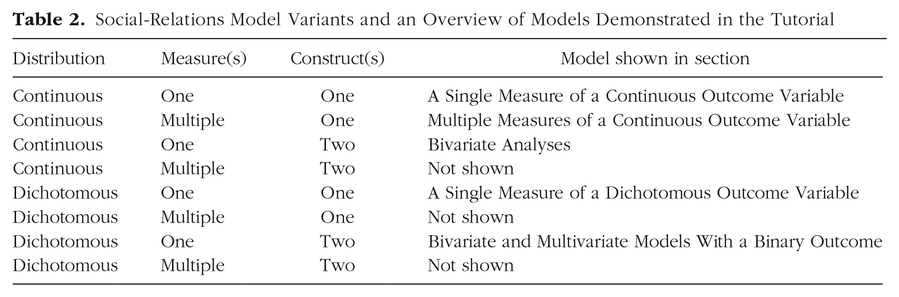
Figure 3 presents the output of only one out of several SRM variations of the asymmetric block design (A Single Measure of a Dichotomous Outcome Variable). To determine the specific variation that needs to be used, one must consider (a) the distribution of the analyzed variable or variables (e.g., continuous, binary ⁵ ), (b) whether more than one measure is available to allow separation of dyadic variance from error variance, and (c) whether more than one variable (construct) is measured in the design. Of the eight possible combinations of these considerations, we show five in this tutorial (see Table 2).

Table 2.

Social-Relations Model Variants and an Overview of Models Demonstrated in the Tutorial

Distribution	Measure(s)	Construct(s)	Model shown in section
Continuous	One	One	A Single Measure of a Continuous Outcome Variable
Continuous	Multiple	One	Multiple Measures of a Continuous Outcome Variable
Continuous	One	Two	Bivariate Analyses
Continuous	Multiple	Two	Not shown
Dichotomous	One	One	A Single Measure of a Dichotomous Outcome Variable
Dichotomous	Multiple	One	Not shown
Dichotomous	One	Two	Bivariate and Multivariate Models With a Binary Outcome
Dichotomous	Multiple	Two	Not shown

Software

Estimating the SRM parameters for data based on an asymmetric block design can be achieved with a program called BLOCKO, which is based on an analysis of variance (ANOVA; Kenny & Xuan, 2013), and with a crossed-mixed-effect model (also known as cross-classified hierarchical models, or just a particular case of a multilevel model [MLM]) using standard software, such as SPSS or SAS (for SPSS examples, see Ackerman et al., 2015). Among the advantages of BLOCKO are automatic computation of the SRM parameters and estimation of the reliabilities of the actor and partner components. BLOCKO, because of its ANOVA approach, has four significant limitations: It does not handle missing data; if there is more than one group, it requires identical group sizes; when population variance is zero, it may yield negative but impossible variance estimates; and it does not integrate fixed-effect parameters seamlessly. These limitations are overcome by specifying the SRM using an MLM (Ackerman et al., 2015). However, with large samples, the MLM code for SPSS can take more than 24 hr to converge (Kluger & Malloy, 2019), and its output is not readily interpretable regarding the SRM estimates. A solution to these limitations is available in R (R Core Team, 2023). Yet the main packages used for mixed effects in R—lme4 (Bates et al., 2015) and nlme (Pinheiro et al., 2023)—lack the flexibility needed for our purpose. The newer glmmTMB package (Brooks et al., 2017) and the brms package (Bürkner, 2017) build on lme4 syntax and do provide the necessary flexibility. Therefore, we show how to use them to estimate the SRM parameters for data from an asymmetric block design. Our codes converge rapidly (glmmTMB with our data set runs under a minute, and brms runs under 10 min for the most demanding model tested here) and tabulate the MLM output consistent with SRM logic. Note that Tu et al. (2022) already used glmmTMB for analyzing asymmetric block design data. In A Single Measure of a Continuous Outcome Variable section, we use a similar code with added explanations. In the remaining sections, we show how to use glmmTMB and brms for more challenging models. ⁶

The Data Set Used for the Example

Appendix A in the Supplemental Material available online provides all the information required to set up the data, packages, and functions to replicate this entire tutorial.

Participants

In fall 2007, 94 men and 93 women (N = 187), all undergraduate students attending Northwestern University, participated in one of eight heterosexual speed-dating events; age: M = 19.6 years (SD = 1.2); 129 participants described themselves as White or Caucasian, 29 described themselves as Asian/Asian American/Chinese/Korean/Taiwanese/Pacific-Islander, 12 described themselves as multiracial or a combination of two or more races/ethnicities, six described themselves as Indian/Asian Indian, five described themselves as Hispanic/Latino, three described themselves as Black/African American, one described themselves as Arab, and the remaining two participants declined to respond.

Procedure

Participants learned of the speed-dating events via posted flyers and informational emails. Interested participants went to a website to sign up for one of four events for freshmen/sophomores or four events for juniors/seniors. They then completed a 30-min intake questionnaire online (for which they were paid $5). Approximately 11 days later, they attended the event in an art gallery in the student union. At the event, participants met 11 to 12 members of the other gender. After each 4-min speed date, all the men (four events) or all the women (four events) stood up and rotated to the next table; all participants then completed a 2-min questionnaire about the date that had just concluded. At the end of the event, participants returned to the website to indicate which of their speed-dating partners they would (“yes”) or would not (“no”) like to exchange contact information with (date again). Twenty-four hours after the event, participants were informed of their matches and provided with the means to contact one another.

Measures

For demonstration purposes, we chose four variables: the order in which the dates took place (e.g., the first dating round, the second); two Likert-scale items taken from the 2-min questionnaire, that is, “physically attractive” and “sexy/hot”; and the dichotomous indication of whether they wanted a second date.

Data

We share a copy of the demonstration data on the OSF site (https://osf.io/vuen2/). These data have been used in multiple publications (Baxter et al., 2022; Eastwick et al., 2010, 2011, 2023; Eastwick & Finkel, 2011; Finkel & Eastwick, 2009; Herrenbrueck et al., 2018; Hopwood et al., 2021; Ireland et al., 2010; Joel et al., 2017; Tidwell et al., 2012; Vacharkulksemsuk et al., 2016), but the analyses of these data shown here were not published previously. The organization of the data set makes it amenable to SRM analyses using an MLM—that is, the data set is organized in a long as opposed to a wide format with identification variables (i.e., identification codes for groups, actors, and partners and a variable identifying the membership in one of the two interacting groups). Next, we show all the variables used in our examples (Table 3) and a sample of the data (Table 4). Note that in Table 4, Actor 19 gave identical attractive and sexy ratings for five partners, but she used different ratings for Partner 302 (across this data set, the zero-order correlation between these items is .90, but less than half of the ratings are identical).

Table 3.

Input Variables

Variable name	Explanation
gID	ID of the speed-dating session (group)
actorID	ID of the actor offering the date
partnerID	ID of the partner who was offered a date
order	The order in which the dates took place (e.g., the first dating round, the second)
gender	Gender of the actor offering the date (f = woman; m = man)
date.again	DV: actorID indications of whether (1 = yes) or not (0 = no) they wanted to exchange information with partnerID (i.e., interested in dating again)
attractive	DV: actorID ratings of partnerID as phsyically attractive on a scale from 1 to 9
sexy	DV: actorID ratings of partnerID as sexy/hot on a scale from 1 to 9

Note: DV = dependent variable.

Table 4.

Example Data of Input Variables

gID	actorID	partnerID	order	gender	date.again	attractive	sexy
1	19	102	9	f	1	5	5
1	19	194	3	f	1	5	5
1	19	275	4	f	0	1	1
1	19	281	11	f	1	3	3
1	19	302	1	f	1	8	7
1	19	303	5	f	1	5	5

Preparing codes for SRM analysis of asymmetric-block-design data

We take four steps to prepare the data for the analyses: (a) creating codes to be used in the specification of the models (a mandatory step), (b) reinspecting the data (a recommended step for checking accuracy), (c) centering fixed variables (needed only if fixed variables are used), and (d) adding pairwise variables (needed only if one plans to regress the behavior of the actor on the partner’s behavior). We illustrate each of these steps below.

Create codes necessary for modeling SRM for asymmetric block design

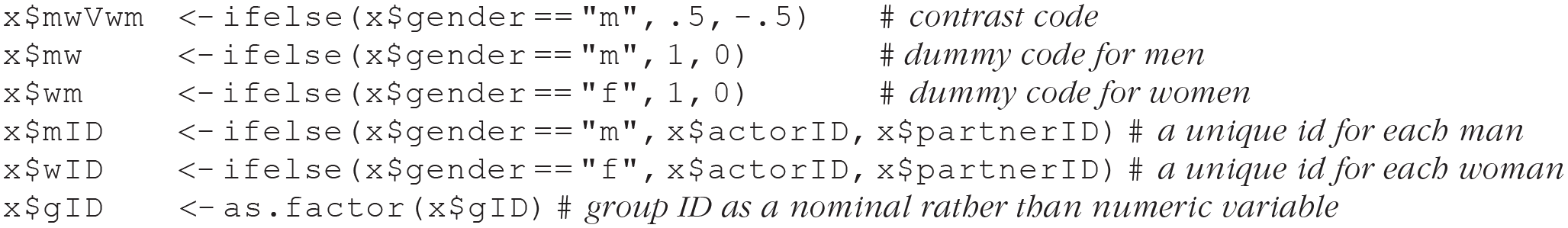
Modeling SRM for asymmetric block design with an MLM requires preparing five codes. One is a contrast code for gender, which allows for testing the fixed effect of gender (or any other variable indexing the two social categories represented in the design). Two are redundant dummy codes representing the source of the data (the actor or the partner) and in our case, whether the data source is men’s reaction to women or vice versa. This set of codes allows proper specification of the random-effects structure. Finally, a pair of ID codes identify the IDs of the actor and the partner and in our case, for each datum, the ID of the man and the ID of the woman involved in the specific interactions. These ID codes allow proper specification of the data as nested within men or women. The preparation of these five R codes is shown next:

Center order on the first interaction (set the first round to zero)

In a typical SRM analysis, the order of the interactions among dyads is ignored. Yet this data set has information about interaction order. A score of 1 means that the data reflect reactions in the first round with an opposite-sex partner in the speed-dating session. We use this variable to demonstrate how investigation of order can be added to the MLM. To increase its interpretability, we subtract 1 from this variable to set the first round to zero. Consequently, the intercept will reflect the outcome variable score at the first round. If the fixed variable has a meaningful mean, then centering can be done by subtracting the mean:

x$order <- x$order - 1

Reinspect the data after adding new variables and manipulating order

The first six rows for woman 19 as an actor. Table 5 shows the same data as Table 4 after adding the new variables, subtracting 1 from order, and rearranging the data by order. It shows a woman with ID 19 (gender = f) met a man with ID 302 in the first round (coded 0). She offered him a second date (date.again = 1) and found him attractive (8) and sexy (7). Her mwVwm code is −0.5 because −0.5 represents women and 0.5 represents men. Note that her wID and mID scores are identical to her actorID and partnerID scores, respectively. For women, the actorID = wID, and for men, actorID = mID; for women, the partnerID = mID, and for men, partnerID = wID.

Table 5.

Coded Variables Added: Actor Focus

gID	actorID	partnerID	order	gender	date.again	attractive	sexy	mwVwm	mw	wm	mID	wID
1	19	302	0	f	1	8	7	−0.50	0	1	302	19
1	19	386	1	f	1	6	6	−0.50	0	1	386	19
1	19	194	2	f	1	5	5	−0.50	0	1	194	19
1	19	275	3	f	0	1	1	−0.50	0	1	275	19
1	19	303	4	f	1	5	5	−0.50	0	1	303	19
1	19	305	5	f	1	6	5	−0.50	0	1	305	19

The first six rows for woman 19 as a partner. Table 6 shows a man with ID 302 (gender = 1) who met a woman with ID 19 in the first round (coded 0). He did not offer her a second date (date.again = 0), and he rated her attractiveness and sexiness only 3 and 2, respectively, on a scale from 1 to 9. His mwVwm code is 0.5. Note that his mID and wID scores are identical to his actorID and partnerID scores, respectively.

Table 6.

Coded Variables Added: Partner Focus

gID	actorID	partnerID	order	gender	date.again	attractive	sexy	mwVwm	mw	wm	mID	wID
1	302	19	0	m	0	3	2	0.50	1	0	302	19
1	386	19	1	m	0	2	2	0.50	1	0	386	19
1	194	19	2	m	1	6	5	0.50	1	0	194	19
1	275	19	3	m	0	2	2	0.50	1	0	275	19
1	303	19	4	m	0	1	1	0.50	1	0	303	19
1	305	19	5	m	0	2	2	0.50	1	0	305	19

Create pairwise variables

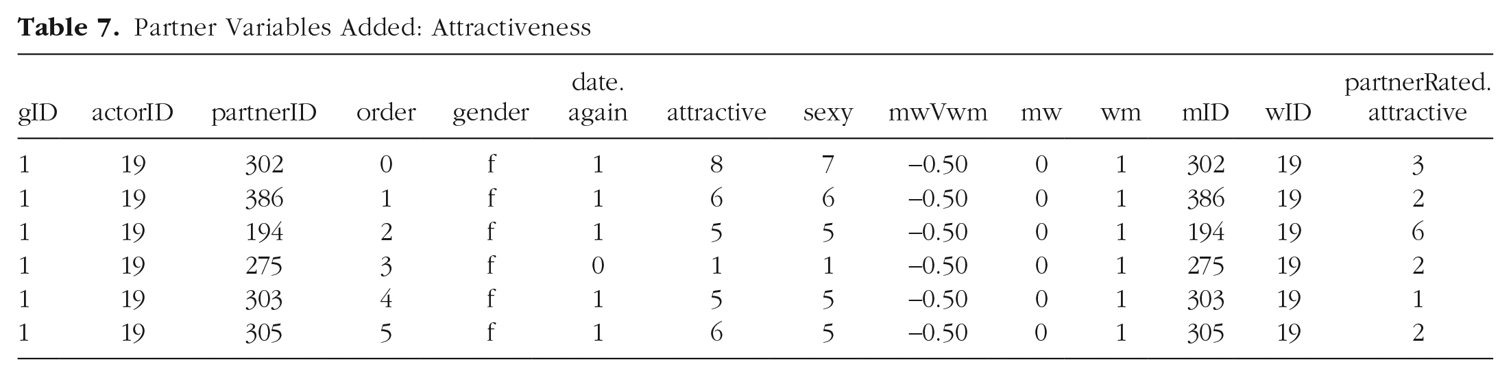
Sometimes, a researcher may wish to use information from the partner to predict behavior of the actor (demonstrated in the Supplemental Material). For that purpose, we wrote a function, pwv, to create a pairwise-data structure (see Appendix B in the Supplemental Material). As an example, we created a variable with the partner’s rating of attractiveness shown in Table 7, which illustrates that the new variable is a copy of the partners’ data reported in Table 6 added to Table 5:

x <- pwv("attractive", "partnerRated.attractive", x)

Table 7.

Partner Variables Added: Attractiveness

gID	actorID	partnerID	order	gender	date.again	attractive	sexy	mwVwm	mw	wm	mID	wID	partnerRated.attractive
1	19	302	0	f	1	8	7	−0.50	0	1	302	19	3
1	19	386	1	f	1	6	6	−0.50	0	1	386	19	2
1	19	194	2	f	1	5	5	−0.50	0	1	194	19	6
1	19	275	3	f	0	1	1	−0.50	0	1	275	19	2
1	19	303	4	f	1	5	5	−0.50	0	1	303	19	1
1	19	305	5	f	1	6	5	−0.50	0	1	305	19	2

Specifying the SRM for an Asymmetric Block Design in R With the glmmTMB Package: An Overview

To specify the SRM for an asymmetric block design in R, we use the glmmTMB package, which, unlike the lme4 and nlme packages, enables simultaneous specification of crossed random effects and a covariance structure for the lower-level residuals. As we show, this is accomplished by fixing the dispersion parameter to a small value close to zero to force the residual variance into the random effects. Although the glmmTMB package was developed to specify generalized linear-mixed models, it can also easily handle linear-mixed models (e.g., Gaussian family with identity link).

Unlike SPSS, glmmTMB does not currently provide approximate denominator degrees of freedom (e.g., the Satterthwaite approximation to degrees of freedom). Thus, the tests of the fixed effects are asymptotic z tests, which usually result in slightly lower p values from programs that compute degrees of freedom (e.g., SAS and SPSS). For additional information about computing p values in an MLM, see Bates et al. (2015).

A single measure of a continuous outcome variable

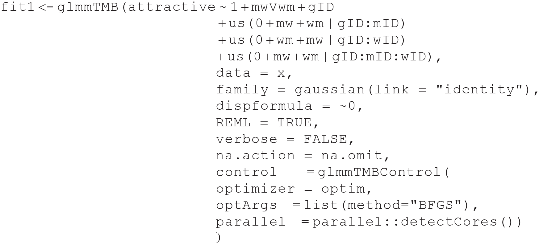
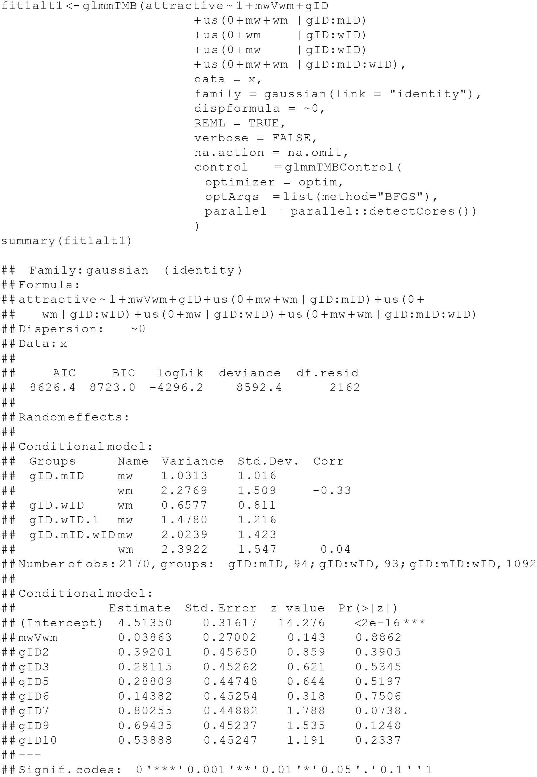
Below is the glmmTMB (Brooks et al., 2017) syntax for estimating the SRM for asymmetric-block-design data when there is a single measure of a continuous outcome variable, in this case, attractiveness:

The syntax shows that we are saving the results of the glmmTMB analysis to an R object called “fit1.” The first argument is the formula: attractive ~ 1 + mwVwm + gID + us(0 + mw + wm | gID:mID) + us(0 + wm + mw | gID:wID) + us(0 + mw + wm | gID:mID:wID). It specifies the fixed and random effects for the mixed-effects model. The term to the left of the tilde (~) should be read as “attractive is regressed on.” The 1 to the right of the tilde requests that glmmTMB estimate the intercept. It can be dropped without consequence because the intercept is estimated by default in glmmTMB. mwVwm requests estimation of the fixed effects of gender, and gID creates a set of k– 1 dummy codes (where k is the number of groups) and estimates whether the groups differ from the reference group. Note that gID must be defined as a factor, or else, it will be considered as a continuous variable, which is meaningless in this context (i.e., there is no reason to believe that there is a linear relationship between the group numbers, such as 1, 2, and 3, and the outcome).

Typically in SRM studies, group variance is negligible because groups are usually sampled from the same population. In such cases, group means are likely to be close to that population mean, and their variance may be only a nuisance that may or may not need to be accounted for. Yet there may be situations in which the researcher expects group variance. For example, in the context of speed dating, it may be that groups of participants in their 20s will show different mean attractiveness ratings compared with speed-dating events for people in their 50s. If one decides to model group variance and if k≥ 20, the group variance should be modeled as a random variable (Snijders & Bosker, 2012, p. 48). If k ≤ 20 but k≥ 10, there are no clear guidelines, and theory can help; if k ≤ 10, group variance should be modeled as fixed, as we do here with eight groups. Yet theory may suggest (e.g., range of age groups) that it is sensible to fit group variance as a random variable when there is a small number of groups (for considerations, see Gelman & Hill, 2007, Section 12.6). To model group variance as a random variable, replace the term gID with (1 | gID); or if one is interested in modeling group variance separately for each group (gender) and their covariance, replace gID with us(0 + mw + wm | gID), consistent with the statistical model in the Appendix.

The following three code lines specify the variance–covariance matrices for the random effects. The argument us next to each parenthetical statement requests an unstructured variance–covariance matrix in which all variances and correlations are freely estimated. The 0 at the beginning of each parenthetical statement suppresses the intercept so that separate random effects for men and women can be specified. This specification is needed with two distinguishable subgroups, as in our case of an asymmetric block design. Furthermore, the grouping variable (or variable combinations in our case) is specified after the | symbol.

The first two lines of random-effect statements specify variance–covariance matrices for each social category at the individual (upper) level. They permit men’s actor and partner effects (mw and wm, respectively) to randomly vary across men within groups (i.e., |gID:mID) and women’s actor and partner effects (wm and mw, respectively) to randomly vary across women within groups (i.e., |gID:wID). Note, however, that the men’s partner effect in the first block, wm, indicates the difference among women in the way they affect men. The final random-effect statement specifies the variance–covariance matrix for the relationship (lower) level. It permits the man-to-woman and woman-to-man relationship effects (mw and wm, respectively) to vary randomly across specific combinations of men and women within groups (i.e., gID:mID:wID).

The argument data = x specifies the object containing the raw data. The argument family = gaussian(link = "identity") requests estimating a linear mixed-effects model by specifying the family as Gaussian (i.e., normal) and the link function as identity, which is used for linear models. The argument dispformula = ~ 0 forces the residual variance to be close to zero. This argument forces the residual variance into the other random effects, enabling us to specify the covariance structure for the lower-level residuals. ⁷

The argument REML = TRUE specifies using restricted maximum likelihood estimation. REML is the default in glmmTMB. If one needs maximum likelihood estimation instead, REML = FALSE should be specified. The argument verbose = FALSE prevents progress information from being printed. The argument na.action = na.omit specifies that we want to drop missing observations from the analysis.

Finally, without the argument control = glmmTMBControl(optimizer = optim, optArgs=list(method="BFGS")), glmmTMB will issue a warning: Warning: Model convergence problem; false convergence (8). See vignette('troubleshooting'). Following the example in https://cran.r-project.org/web/packages/glmmTMB/vignettes/troubleshooting.html, we used the nondefault optimizer. Nevertheless, the results of the default optimizer and the BFGS are very similar (see Appendix C in the Supplemental Material), suggesting that the problem stems from the glmmTMB default optimizer and not our model. We observed the same inconsequential error using a different data set not reported here.

We also added to the control argument parallel = parallel::detectCores(). This argument uses the package parallel, which is part of R, that detects how many cores the computer has and assigns the modeling to all available cores to allow parallel processing. This argument speeds up the estimation of the model.

The syntax below prints the results stored in fit1:

Interpretation of the results

The initial portions of the output from the summary function show the mixed-effects model equation for the analysis and several fit statistics (e.g., the deviance). Below the model equation are the results for the random effects organized by block. The first block (i.e., for the grouping variable combination, gID:mID) shows the estimates for men’s actor effect variance (1.03), men’s partner effect variance (2.28), and men’s generalized reciprocity or the correlation of a man’s actor effect with his partner effect (–0.33). The second block (i.e., for the grouping variable combination, gID:wID) shows the estimates for women’s actor effect variance (0.66), women’s partner effect variance (1.47), and women’s generalized reciprocity (–0.13). The final block (i.e., for the grouping variable combination, gID:mID:wID) shows the estimates for the man-to-woman relationship effect variance (2.02), the woman-to-man relationship effect variance (2.39), and relationship reciprocity (0.04).

After this, the output shows the total number of observations in the study (2,170) and the number of observations for each grouping variable (i.e., 94 men within groups, 93 women within groups, and 1,092 man–woman pairings within groups). The output for the fixed effects follows; it is discussed below.

To facilitate the interpretation of this output, we wrote two functions to extract, rearrange, and tabulate the results: tabulateSRM.fixed tabulates the fixed effects, and tabulateSRM.rand.uni tabulates the random effects for a model with a single outcome (univariate). The functions extract information from the outputs of the glmmTMB’s helper functions summary and confint and calculate the standardized estimates of the variances. The functions are provided in Appendix D in the Supplemental Material.

The fixed effects

tabulateSRM.fixed(fit1, caption = "Fixed Effects")

The intercept for the fixed effects in Table 8 shows that the average person in Group 1 rated the attractiveness as 4.51. The estimate for the effect of mwVwm shows that men rated the attractiveness of women (i.e., 4.51 + [0.5 × 0.04], or 4.53) higher than women rated men’s attractiveness(i.e., 4.51 − [0.5 × 0.04] or 4.49), but the difference was not statistically significant, p = .89. The subsequent terms compare group means with Group 1 (set as the intercept). They show that in Group 2, people rated attractiveness 0.39 higher than in Group 1, and in Group 3, people rated attractiveness 0.28 higher than in Group 1, and so on; all differences from Group 1 are statistically insignificant.

Table 8.

Fixed Effects

		95% confidence interval
Variable	Estimate	Lower bound	Upper bound	p
(Intercept)	4.51	3.91	5.12	< .001
mwVwm	0.04	−0.50	0.58	.889
gID2	0.39	−0.48	1.26	.377
gID3	0.28	−0.58	1.14	.523
gID5	0.29	−0.57	1.14	.509
gID6	0.14	−0.72	1.01	.743
gID7	0.80	−0.05	1.66	.066
gID9	0.69	−0.17	1.56	.114
gID10	0.54	−0.32	1.40	.220

The random effects

tabulateSRM.rand.uni(fit1, caption = "Random Effects")

We reorganized the information about random effects extracted from the glmmTMB output with the tabulateSRM.rand.uni function in Table 9 and added statistical notations to help map the names of the model’s components to the formal model presented in the Appendix. In Appendix D in the Supplemental Material, we show how to use the tabulateSRM.rand.uni function to print the table without or with these symbols. We also show in the Supplemental Material how to tabulate all other models without and with statistical notation.

Table 9.

Random Effects

			95% confidence interval
Component	Symbol	Estimate	Lower bound	Upper bound	Standardized
Men
Actor variance	${\mathrm{\sigma }}_{\mathrm{\alpha }A}^2$	1.03	0.73	1.46	22.8%
Partner variance	${\mathrm{\sigma }}_{\mathrm{\beta }B}^2$	1.47	1.06	2.06	32.5%
Relationship + error variance	${\mathrm{\sigma }}_{\mathrm{\gamma }A}^2$	2.02	1.85	2.22	44.7%
Actor–partner correlation	${\mathrm{\sigma }}_{\mathrm{\alpha }\mathrm{\beta }A}$	−.33	−.51	−.09
Women
Actor variance	${\mathrm{\sigma }}_{\mathrm{\alpha }B}^2$	0.66	0.44	0.97	12.3%
Partner variance	${\mathrm{\sigma }}_{\mathrm{\beta }A}^2$	2.28	1.65	3.14	42.8%
Relationship + error variance	${\mathrm{\sigma }}_{\mathrm{\gamma }B}^2$	2.39	2.18	2.62	44.9%
Actor–partner correlation	${\mathrm{\sigma }}_{\mathrm{\alpha }\mathrm{\beta }B}$	−.13	−.36	.13
Relationship correlation	${\mathrm{\sigma }}_{\mathrm{\gamma }\mathrm{\gamma }}$	.04	−.03	.11

The statistical notation can be read without reading the Appendix. Specifically, the ${\mathrm{\sigma }}^2$ symbols indicate variances, $\mathrm{\sigma }$ indicates covariances, $\mathrm{\alpha }$ indicates actor, $\mathrm{\beta }$ indicates partner, $\mathrm{\gamma }$ indicates relationship (with error), A indicates one social group (men in Table 9), and B indicates the other social group (women).

Most notably, we place the women’s partner effect, ${\mathrm{\sigma }}_{\mathrm{\beta }B}^2$ , in the men’s results and the men’s partner effect in the women’s results. This choice is needed to standardize the variances in a meaningful way. That is, men’s behavior is driven by their traits as actors, by women’s traits as partners, and by their relationship behavior toward each woman. Therefore, Table 9 shows that for men, the men’s actor, women’s partner, and error variances were 1.03, 1.47, and 2.02, respectively. The lower bounds of the confidence interval of the actor and partner variances are far from zero, and the confidence interval appears almost symmetric about the estimate, suggesting that these variances are not negligible. Yet below, we show how to test the statistical significance of the variance by removing it from the model and comparing a model with it (i.e., full) and a model without it (i.e., restricted).

Next, the total variance for men is 1.03 + 1.47 + 2.02. Therefore, the males’ actor variance accounts for $\left(\frac{1.03}{1.03+1.47+2.02}\right)$ of the males’ total variance, or 22.8%, as shown in Table 9 as a standardized value. The actor–partner correlation is negative for both sexes but significant only for men because the confidence interval for women included zero. This suggests that the more a man rates all women, on average, as attractive, the less all women, on average, find him attractive. Last, the positive relationship correlation suggests that a participant who finds a specific partner more attractive is also perceived by that partner as more attractive, but this effect is negligible and nonsignificant.

It is possible to test the significance of the reciprocities by removing them from the model and comparing full and restricted models. For example, we can remove the actor–partner correlation for women by specifying the actor and the partner components nested within gID:wID separately so their covariance would not be estimated. We show this analysis and its results below. The actor–partner correlation for women is assumed to be zero and not printed. The estimate for the women partner effect changes slightly.

Next, we can compare fit1 with fi2alt1.

Dropping the actor–partner correlation for women only slightly worsens the fit, and the difference between the models is nonsignificant. This suggests that the actor–partner correlation for women is nonsignificant, p = .317. It is now possible to drop any women variance from the model (e.g., the partner variance) and test whether it is significant as follows. However, dropping the partner variance also entails dropping the correlation just tested, creating a model that has two more degrees of freedom. Thus, the model without partner variance needs to be compared with the model without the actor–partner correlation, as shown below:

This time, dropping a term worsened the fit substantially, suggesting that the partner variance for women is significant and a required term in the model. Finally, below, we illustrate a parallel analysis for the men. It shows that dropping the actor–partner correlation worsened the fit substantially, suggesting that the actor–partner correlation is significant, consistent with the confidence interval in Table 9:

Multiple measures of a continuous outcome variable

When more than one measure of the same construct is available, we can separate relationship (dyadic) and error variances. As an example, we could treat the measures of attractive and sexy as indicators of a general construct of attractiveness.

Pivot the data set (stacking)

To model SRM parameters for an outcome that is a construct indexed by multiple indicators with an MLM, the data set needs to be rearranged to consider the measures (Measure 1, Measure 2, etc.), or indicators, as a random variable. In our example, we presume that the items attractive and sexy are indicators of the construct of attractiveness. Following the pivoting code, ⁸ we show in Table 10 the first 12 rows of the pivoted data frame. Note the new columns: “indicator” and “value.” The indicator column is a character variable that takes the names of the measures as values (e.g., attractive). This column would be one of the random variables in the model. The value column is a numeric variable containing the response to the relevant item. This column would be the dependent variable of the model:

Table 10.

Long Format With Attractiveness Item as Values of the Variable Indicator

gID	actorID	partnerID	gender	mwVwm	mw	wm	mID	wID	indicator	value	attractiveDummy	sexyDummy	mw.attractive	wm.attractive	mw.sexy	wm.sexy
1	19	102	f	−0.50	0	1	102	19	attractive	5	1	0	0	1	0	0
1	19	102	f	−0.50	0	1	102	19	sexy	5	0	1	0	0	0	1
1	19	194	f	−0.50	0	1	194	19	attractive	5	1	0	0	1	0	0
1	19	194	f	−0.50	0	1	194	19	sexy	5	0	1	0	0	0	1
1	19	275	f	−0.50	0	1	275	19	attractive	1	1	0	0	1	0	0
1	19	275	f	−0.50	0	1	275	19	sexy	1	0	1	0	0	0	1
1	19	281	f	−0.50	0	1	281	19	attractive	3	1	0	0	1	0	0
1	19	281	f	−0.50	0	1	281	19	sexy	3	0	1	0	0	0	1
1	19	302	f	−0.50	0	1	302	19	attractive	8	1	0	0	1	0	0
1	19	302	f	−0.50	0	1	302	19	sexy	7	0	1	0	0	0	1
1	19	303	f	−0.50	0	1	303	19	attractive	5	1	0	0	1	0	0
1	19	303	f	−0.50	0	1	303	19	sexy	5	0	1	0	0	0	1

MLMs for multiple indicators

When modeling SRM with multiple indicators, variance partitioning is separated into two parts (Kenny, 1994). The first part is variance shared across the multiple measures, referred to as “stable” variance. The second part is variance not shared across measures, referred to as “unstable” variance. To accomplish this within glmmTMB, the MLM below is an extension of the MLM we used to estimate a model for an outcome based on a single measure (fit1). The difference between the models is the addition of three terms, us(0 + mw + wm | gID:mID:indicator) + us(0 + wm + mw | gID:wID:indicator) + us(0 + mw + wm | gID:mID:wID:indicator), estimating error variance for each of the SRM components. These terms are similar to the first three random terms, us(0 + mw + wm | gID:mID) + us(0 + wm + mw | gID:wID) + us(0 + mw + wm | gID:mID:wID), and differ only by the addition of nesting in the :indicator. The estimates of the variance within the indicators reflect the unstable or unreliable variance components stemming from differences between the items indicating the construct (the attractive and sexy items). Another minor difference is that we dropped the fixed effect of the groups, gID, because it was insignificant, so we can save some space.

Interpretation of the results

The output organizes the random effects by block. The first block (i.e., for the grouping variable combination, gID:mID) shows the estimates for men’s actor effect variance (0.91), men’s partner effect variance (2.15), and men’s generalized reciprocity (–0.32). The second block (i.e., for the grouping variable combination, gID:wID) shows the estimates for women’s actor effect variance (0.6), women’s partner effect variance (1.54), and women’s generalized reciprocity (–0.25). The third block (i.e., for the grouping variable combination, gID:mID:wID) shows the estimates for the man-to-woman relationship effect variance (1.71), the woman-to-man relationship effect variance (1.82), and relationship reciprocity (0.04). The following three blocks report the unstable variances and their correlations for each of the above components. For example, the unstable men’s actor variance is 0.16. To standardize the variances, the total unstable variances are summed for men and women separately and indicate the total error variance. For example, for men, the total error variance is 0.16 + 0.05 + 0.29, or 0.5. Therefore, the standardized men’s actor variance is their actor variance, 0.91, divided by the sum of their variances, including the women’s partner effect, 1.54, relationship effect, 1.71, and the error, 0.5, that is, $\left(\frac{0.91}{0.91+1.54+1.71+0.16+0.05+0.29}\right)$ = 19.6%.

After this, the output shows the total number of observations in the study (N = 4,340) and the number of observations for each grouping variable (i.e., 94 men within groups, 93 women within groups, 1,092 man–woman pairings within groups, and 2,184 people within indicators). The output for the fixed effects then follows and is discussed below.

The glmmTMB output for the fixed effects is provided at the bottom of the output, and the estimates are interpreted like regression coefficients.

As for previous models, we use two functions to extract, rearrange, and tabulate the results: tabulateSRM.fixed, which was used for the single outcome, tabulates the fixed effects, and tabulateSRM.rand.mv is a new function needed to tabulate the random effects for a model with a latent outcome (multivariate). The tabulateSRM.rand.mv provides estimates of standardized variances by calculating error variance for men and women by summing up all the estimates of the unstable variances. The function is provided in Appendix E in the Supplemental Material.

The fixed effects

tabulateSRM.fixed(fit2, caption = "Fixed Effects of Multi item Outcome")

The intercept for the fixed effects in Table 11 shows that the average person in Group 1 rated partners’ attractiveness at 4.58, as estimated by two indicators (attractive and sexy). The estimate for the effect of mwVwm shows that men found women more attractive (i.e., 4.58 + [0.5 × 0.16] = 4.66) than women found men (i.e., 4.58 − [0.5 × 0.16] = 4.5), but the difference was not statistically significant because the confidence interval includes zero.

Table 11.

Fixed Effects of Multiitem Outcome

		95% confidence interval
Variable	Estimate	Lower bound	Upper bound	p
(Intercept)	4.58	4.36	4.80	< .001
mwVwm	0.16	−0.38	0.70	.557

The random effects

tabulateSRM.rand.mv(fit2, caption = "Random Effects of Multi item Outcome")

The random effects in Table 12 show that the actor, partner, relationship, and error variances for women were 0.6, 2.15, 1.82, and 0.87, respectively. The lower bounds of the confidence interval of the actor, partner, and relationship variances are above zero, suggesting that these variances are significantly higher than zero in the population. Next, the total women’s variance is 0.6 + 2.15 + 1.82 + 0.41 + 0.03 + 0.43. Therefore, the actor variance accounts for 11% of the total variance $\left(\frac{0.6}{0.6+2.15+1.82+0.41+0.03+0.43}\right)$ . The actor–partner correlation is negative for both sexes but significant only for men because the confidence interval for women included zero. This suggests that men who rated, on average, all their women partners as attractive were consistently rated as less attractive by these women, on average. Last, the positive relationship correlation suggests that a participant who rated a specific partner as more attractive than the participant typically rated other partners elicited similar rating from that specific partner, but this effect is negligible and nonsignificant.

Table 12.

Random Effects of Multiitem Outcome

			95% confidence interval
Component	Symbol	Estimate	Lower bound	Upper bound	Standardized
Men
Actor variance	${\mathrm{\sigma }}_{\mathrm{\alpha }A}^2$	0.91	0.62	1.33	19.6%
Women’s partner variance	${\mathrm{\sigma }}_{\mathrm{\beta }B}^2$	1.54	1.11	2.15	33.1%
Relationship variance	${\mathrm{\sigma }}_{\mathrm{\gamma }A}^2$	1.71	1.54	1.89	36.6%
Error variance	${\mathrm{\sigma }}_{ϵA}^2$	0.50			10.7%
Actor–partner correlation	${\mathrm{\sigma }}_{\mathrm{\alpha }\mathrm{\beta }A}$	−.32	−.51	−.08
Women
Actor variance	${\mathrm{\sigma }}_{\mathrm{\alpha }B}^2$	0.60	0.36	0.99	11.0%
Men’s partner variance	${\mathrm{\sigma }}_{\mathrm{\beta }A}^2$	2.15	1.56	2.94	39.5%
Relationship variance	${\mathrm{\sigma }}_{\mathrm{\gamma }B}^2$	1.82	1.64	2.02	33.5%
Error variance	${\mathrm{\sigma }}_{ϵB}^2$	0.87			16.0%
Actor–partner correlation	${\mathrm{\sigma }}_{\mathrm{\alpha }\mathrm{\beta }B}$	−.25	−.49	.05
Relationship correlation	${\mathrm{\sigma }}_{\mathrm{\gamma }\mathrm{\gamma }}$	.04	−.03	.11

Bivariate analyses

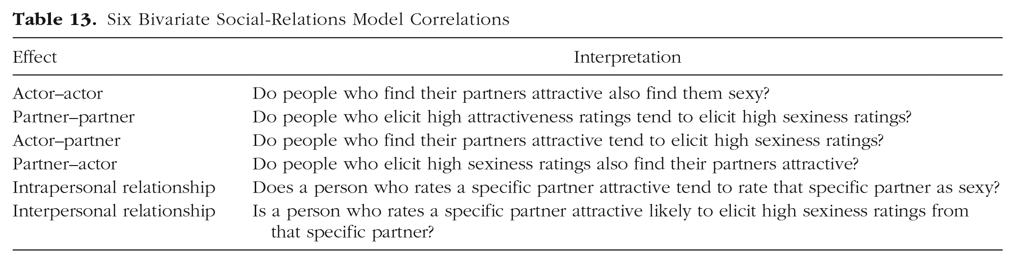
In the previous section, we assumed that the items attractive and sexy are indicators of the same latent variable—attractiveness. Yet one could also assume that they are different constructs. This assumption is not tenable here because the zero-order correlation between these items is .90. Nevertheless, we proceed using the same items to facilitate comparison with the previous section. When two SRM measures are assumed to tap different constructs, researchers are often interested in the correlations between the components of these measures (Kenny et al., 2006). In this context, one can compute six correlations: actor–actor, partner–partner, actor–partner, partner–actor, intrapersonal relationship, and interpersonal relationship. In Table 13, we explain the interpretation of these six effects in the current data context.

Table 13.

Six Bivariate Social-Relations Model Correlations

Effect	Interpretation
Actor–actor	Do people who find their partners attractive also find them sexy?
Partner–partner	Do people who elicit high attractiveness ratings tend to elicit high sexiness ratings?
Actor–partner	Do people who find their partners attractive tend to elicit high sexiness ratings?
Partner–actor	Do people who elicit high sexiness ratings also find their partners attractive?
Intrapersonal relationship	Does a person who rates a specific partner attractive tend to rate that specific partner as sexy?
Interpersonal relationship	Is a person who rates a specific partner attractive likely to elicit high sexiness ratings from that specific partner?

Testing the six questions relies on the stacked data used in the previous section with additional dummy codes. One set of dummy codes represents the different measures (attractive and sexy). The second set of four dummy codes indicates whether each measure involves a man rating a woman or vice versa. Next, the glmmTMB here is an extension of the MLM we used to estimate a model for an outcome based on a single measure above (fit1). The difference between the models is the replacement of the dummy codes for gender. Specifically, the term us(0 + mw + wm | gID:mID) is replaced with dummy codes for gender for each measure: us(0 + mw.attractive + wm.attractive + mw.sexy + wm.sexy | gID:mID).

In addition, rather than testing only the fixed effect of gender, in this model, we test the fixed effects of gender, the measure, and their interactions: 1 + mwVwm × attractiveDummy. If the interaction is significant, we can facilitate its interpretation by replacing the fixed part of the model with 0 + mw:(attractiveDummy + sexyDummy) + wm:(attractiveDummy + sexyDummy), which will print the estimated mean of each measure by gender. The coding of the needed dummy codes and the glmmTMB model are shown next:

Interpretation of the results

The output organizes the random effects by block. The first block (i.e., for the grouping variable combination, gID:mID) shows the estimates for men. Within this block, the first (last) two rows pertain to the univariate results of the attractive item (the sexy item). For example, the first row contains the men’s actor effect variance on the attractive item (1.02), and the second one contains the men’s partner effect variance on the attractive item (2.23) and the men’s generalized reciprocity on the attractive item (–0.32). Note that these estimates are slightly different from those obtained when the attractive item variable is decomposed in a univariate model in A Single Measure of a Continuous Outcome Variable section above with fit1. For example, the estimates in the univariate model are 1.03, 2.28, and −0.33 for men’s actor, partner, and generalized reciprocity. The estimates of the variances and the correlations change slightly with the addition of fixed or random effects to the model.

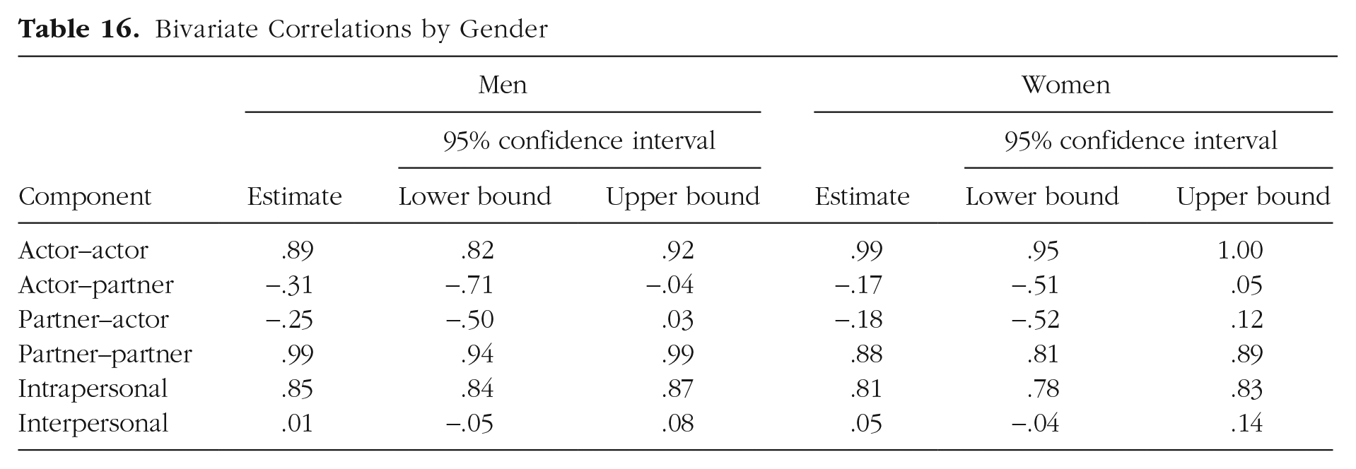
Most important are the correlations between actor, partner, and error + relationship effects of one variable with the other. The first block (for men) shows that the actor–actor correlation is .89 (the more attractive a man rates all women, the more sexy he rates them). The actor–partner correlation is −.31 (the more attractive a man rates all women, the less sexy his women partners find him). The partner–actor correlation is −.25 (the higher attractiveness ratings a man elicits, the lower his ratings of the sexiness of all women). And the partner–partner correlation is .99 (the more a man elicits attractiveness ratings, the more he also elicits sexiness ratings). The second block shows the same parameters for women. Both indicate that the actor–actor and partner–partner correlations approach unity, strongly suggesting that these measures tap the same construct. Note that exceptionally high actor–actor and partner-partner, and even out of bounds, correlations, could be caused by unreliability when at least one correlated component has a small variance (Bonito & Kenny, 2010), but this is not the case here.

The last block presents relationship reciprocities and intrapersonal and interpersonal correlations. Specifically, it shows that the univariate relationship reciprocity for the attractive item is .04 (and .03 for the sexy item), that the intrapersonal correlation for the attractive item is .85 (and .81 for the sexy item), and that the interpersonal correlation for the attractive item is .01 (and .05 for the sexy item). In our case, consistent with the actor–actor and partner–partner correlations, the intrapersonal correlations are very high, suggesting that the two measures reflect the same construct. In addition, in our case, there is no evidence that rating a specific partner high on one item predicts the ratings on the other item by that specific partner.

Finally, as for previous models, we wrote functions to extract, rearrange, and tabulate the results: tabulateSRM.fixed tabulates the fixed effects (the same as for previous models), tabulateSRM.rand.bi tabulates the univariate random effects for a bivariate model, and tabulateSRM.bivariate.cor tabulates the bivariate correlations. The functions are provided in Appendix F in the Supplemental Material. Their respective outputs are shown in Tables 14 through 16.

Table 14.

Fixed Effects of Multiitem Outcome

		95% confidence interval
Variable	Estimate	Lower bound	Upper bound	p
(Intercept)	4.25	4.03	4.48	< .001
mwVwm	0.29	−0.27	0.84	.315
attractiveDummy	0.65	0.57	0.73	< .001
mwVwm:attractiveDummy	−0.25	−0.42	−0.07	.005

Table 15.

Univariate Random Effects of Measures A and B in a Bivariate Model

	Measure 1				Measure 2
		95% confidence interval				95% confidence interval
Component	Estimate	Lower bound	Upper bound	Standardized	Estimate	Lower bound	Upper bound	Standardized
Men
Actor variance	1.02	0.72	1.44	22.4%	1.06	0.75	1.50	22.6%
Partner variance	1.50	1.08	2.09	33.0%	1.67	1.20	2.32	35.5%
Relationship + error variance	2.03	1.85	2.22	44.6%	1.97	1.80	2.16	42.0%
Actor–partner univariate correlation	−.32	−.51	−.09		−.26	−.72	.08
Women
Actor variance	0.65	0.44	0.96	12.4%	1.10	0.78	1.56	20.8%
Partner variance	2.23	1.62	3.06	42.3%	2.10	1.53	2.87	39.4%
Relationship + error variance	2.39	2.18	2.62	45.4%	2.11	1.93	2.32	39.8%
Actor–partner univariate correlation	−.15	−.38	.11		−.18	−.63	.09
Relationship univariate correlation	.04	−.03	.11		.03	−.08	.12

Table 16.

Bivariate Correlations by Gender

	Men			Women
		95% confidence interval			95% confidence interval
Component	Estimate	Lower bound	Upper bound	Estimate	Lower bound	Upper bound
Actor–actor	.89	.82	.92	.99	.95	1.00
Actor–partner	−.31	−.71	−.04	−.17	−.51	.05
Partner–actor	−.25	−.50	.03	−.18	−.52	.12
Partner–partner	.99	.94	.99	.88	.81	.89
Intrapersonal	.85	.84	.87	.81	.78	.83
Interpersonal	.01	−.05	.08	.05	−.04	.14

The fixed effects

tabulateSRM.fixed(fit3, caption = "Fixed Effects of Multi item Outcome")

The fixed effects suggest that attractiveness is rated higher than sexiness. Yet the significant interaction suggests that women rate sexiness lower than men do. This finding can be plotted, as shown below, to facilitate interpretation (Fig. 4):

Fig. 4.

Fixed effects: The interaction between gender and measure.

The random effects

tabulateSRM.rand.bi(fit3, caption =

 "Univariate Random Effects of Measures A and B in a Bivariate Model")

The bivariate correlations

tabulateSRM.bivariate.cor(fit3, caption = "Bivariate Correlations by Gender")

A single measure of a dichotomous outcome variable

We now turn our attention to the date.again outcome variable. This binary variable indicates whether the actor offered a partner a second date (yes = 1, no = 0). Although the glmmTMB function can be adapted to estimate a model in which the dependent variable is dichotomous, it fails to estimate the dyadic reciprocity. Therefore, we use a Bayesian model, using the brms package and its brm function (Bürkner, 2017). ⁹ Below is the syntax for estimating the SRM for asymmetric-block-design data when there is a single measure of a dichotomous outcome variable. Note that this syntax can run for 15 min or more on a slow computer. Therefore, one can test whether the model runs properly by reducing the number of iterations (iter), and only if no syntax error is found can one then run it with a large number of iterations to obtain reliable results. To help the user gauge the convergence time, we preceded the brm function with a measure of starting time and added a command that prints the time elapsed from the start time immediately following the brm. Importantly, modeling dyadic variance in this context requires the addition of a dyad ID code, shown below:

The syntax for the formula for this model is date.again ~ mwVwm + (1 | dyadID) + (mw + wm - 1 | gID:mID) + (wm + mw - 1 | gID:wID). It differs from the one we used to estimate the SRM parameters for a continuous dependent variable in three ways. First, the formula does not contain a term to estimate the residual (relationship) variances because the error variance of a logistic regression model is fixed to equal π≈ 3.29 (e.g., Norton & Dowd, 2017). Second, we add a term to estimate dyadic variance (1 | dyadID). The dyadic variance allows the estimation of dyadic reciprocity, and it equals $\frac{\mathrm{Dyad}\mathrm{variance}}{\mathrm{Dyad}\mathrm{variance}+\mathrm{Error}\mathrm{variance}}$ (Koster, 2020; Snijders & Kenny, 1999); for a binary outcome, it is $\frac{\mathrm{Dyad}\mathrm{variance}}{\mathrm{Dyad}\mathrm{variance}+3.29}$ . Yet this dyadic variance is not included in the variance partitioning because it is an estimate across the two social categories (e.g., men and women).

Third, the argument family = bernoulli(link="logit") requests a generalized linear mixed-effects model by specifying the family as Bernoulli (i.e., binary) and the link function as logit. A logit is a logarithm of the odds, where the odds equals $\frac{p}{1-p}$ . We do not include the fixed group effect because none of the dummy codes significantly differs from the intercept. In addition, we increased the number of iterations from 2,000 (the default) to 8,000 because with the default, we got (R-hat) values larger than 1.00, which indicates poor convergence. ¹⁰

Finally, the argument cores = parallel::detectCores() is especially useful here because the Bayesian model takes an appreciatively longer time to converge than the previous models. In our example, this argument can cut the estimation time from 10 min to just more than 5 min on a computer with eight cores. In more complex models, which take longer to converge, the benefit of this argument grows. We added a time measure for this analysis, which can be safely removed (startTime <- Sys.time() before the code and Sys.time() - startTime) following it.

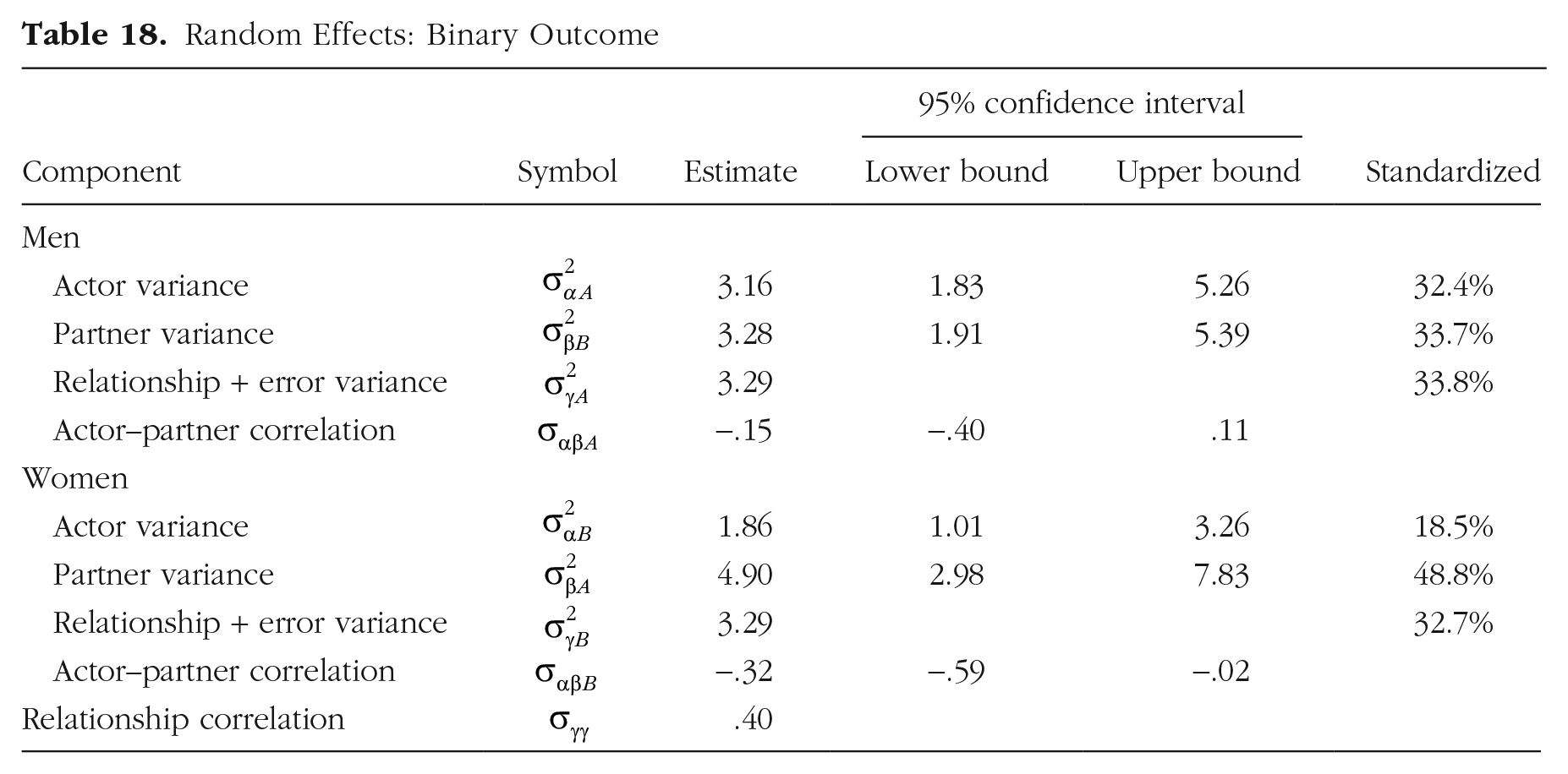
Printing object fit4 provides estimation of standard deviations, rather than the variances, of the random components of the model, along with the standard error and confidence intervals. The values of R-hat for all parameters = 1.00, indicating that the model converged properly. To extract the random and fixed effects from fit4, one can use the helper functions VarCorr(fit4) and fixef(fit4), respectively. Using VarCorr(fit4), we extracted the standard deviation of the dyad ID, squared it to obtain its variance, and used it to calculate dyadic reciprocity with dyadVar/(dyadVar + (pi^2)/3), which yields .40. However, this will work only if the dyadic reciprocity is positive. We show how to estimate negative dyadic reciprocity in Appendix G in the Supplemental Material. ¹¹

It is possible to test the significance of the dyadic variance by dropping it from the model, running the new model, fit4alt, and comparing its results with the results of the original model, fit4. Specifically, for each model, one can compute the model fit with LOO—leave-one-out cross-validation—and compare the LOOs with a measure of the difference in expected log pointwise predictive density (ELPD) between the two models. When the ELPD > |4| and the sample size > 100, as is the case here, the standard error can be used to assess whether the two models differ (Sivula et al., 2020). ¹²

Interpretation of the results

To aid interpretation, we wrote two functions to extract, rearrange, and tabulate the results: tabulateSRM.fixed.bin tabulates the fixed effects, and tabulateSRM.rand.bin tabulates the random effects for a model with a single binary outcome. The function is provided in Appendix H in the Supplemental Material.

The fixed effects

tabulateSRM.fixed.bin(fit4, "Fixed Effects: Binary Outcome")

The fixed-effects results are presented in Table 17 in logit units. We can extract them and convert them to probabilities:

Table 17.

Fixed Effects: Binary Outcome

		95% confidence interval
Variable	Estimate	Lower bound	Upper bound	p
Intercept	−0.35	−0.73	0.01	.032
mwVwm	−0.23	−1.10	0.62	.301

The model estimates that the average person with an mwVwm score of zero (no one) offers a second date to 41.3% of partners. Yet males are less likely to offer a second date, 38.6%, than females, 44.1%.

The random effects

The brm output in Table 18 for binary outcome does not estimate error variance. Instead, the error variance of a model with a binary outcome is fixed at $\frac{{\pi }^2}{3}$ ≈ 3.29 for each group. Therefore, the standardized actor variance estimate for men, for example, is $\frac{3.16}{3.16+4.9+3.29}$ = 27.8%. The actor effects indicate the degree of variance in eagerness. Some participants offer many second dates, and some people offer a few second dates. The partner effects indicate the degree of variance in attractiveness. Some participants received many offers, and some received few. The actor–partner correlation indicates, for both sexes, that eager people are less attractive or that attractive people are less eager. A visual representation of these results is shown in Figure 3. Yet note that the proportion of the actor and partner variances for men and women cannot be compared here because the error variance is set to be equal ( $\frac{{\pi }^2}{3}$ ≈ 3.29). If they are not equal, the comparison of variance proportion across men and women is misleading:

tabulateSRM.rand.bin(fit4, digit = 2, "Random Effects: Binary Outcome")

Table 18.

Random Effects: Binary Outcome

			95% confidence interval
Component	Symbol	Estimate	Lower bound	Upper bound	Standardized
Men
Actor variance	${\mathrm{\sigma }}_{\mathrm{\alpha }A}^2$	3.16	1.83	5.26	32.4%
Partner variance	${\mathrm{\sigma }}_{\mathrm{\beta }B}^2$	3.28	1.91	5.39	33.7%
Relationship + error variance	${\mathrm{\sigma }}_{\mathrm{\gamma }A}^2$	3.29			33.8%
Actor–partner correlation	${\mathrm{\sigma }}_{\mathrm{\alpha }\mathrm{\beta }A}$	−.15	−.40	.11
Women
Actor variance	${\mathrm{\sigma }}_{\mathrm{\alpha }B}^2$	1.86	1.01	3.26	18.5%
Partner variance	${\mathrm{\sigma }}_{\mathrm{\beta }A}^2$	4.90	2.98	7.83	48.8%
Relationship + error variance	${\mathrm{\sigma }}_{\mathrm{\gamma }B}^2$	3.29			32.7%
Actor–partner correlation	${\mathrm{\sigma }}_{\mathrm{\alpha }\mathrm{\beta }B}$	−.32	−.59	−.02
Relationship correlation	${\mathrm{\sigma }}_{\mathrm{\gamma }\mathrm{\gamma }}$	.40

The effect of order

Next, we can ask whether eagerness (choosiness) changes as the speed-dating session continues. To test this question, we added the order variable and its interaction with the sex contrast effect to the model’s fixed effects (i.e., instead of mwVwm, we wrote mwVwm × order) and created a fit5 object (not shown). The interaction is significant marginally (Table 19); hence, we plotted the interaction (Fig. 5), which translates the logit estimates into probabilities. As shown in Figure 5, women are more eager than men in the first rounds, but eagerness for both declines round to round and is similar in later sessions:

tabulateSRM.fixed.bin(fit5, "Fixed Effects: Interaction with Order")

Table 19.

Fixed Effects: Interaction With Order

		95% confidence interval
Variable	Estimate	Lower bound	Upper bound	p
Intercept	0.12	−0.33	0.57	.307
mwVwm	−0.53	−1.50	0.42	.140
order	−0.09	−0.14	−0.04	< .001
mwVwm:order	0.05	−0.02	0.13	.086

Fig. 5.

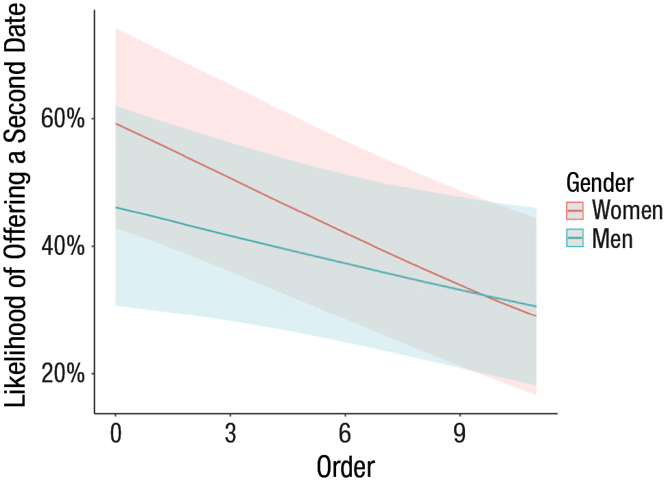
Fixed effects: Likelihood of offering a second date by speed-dating order and gender.

Finally, we note that changing the fixed part of the model changes the random-effects estimates slightly. There is no substantial change, but we point out that the results are not identical.

Bivariate and multivariate models with a binary outcome

Our data raise questions about bivariate correlations between rating of attractiveness and sexiness and second-date offers. As in Bivariate Analysis section above, one can ask six questions about each bivariate correlation. Yet in this case, one SRM variable is continuous (e.g., rating of sexiness), and the other is dichotomous (second-date offers). If one can assume an underlying normal latent variable for the binary response, one may adopt an existing method (Gueorguieva & Agresti, 2001) for the asymmetric block design. Appendix I in the Supplemental Material demonstrates a possible practical work-around. Its drawback is that it may be biased because it treats the components of the predictor (sexiness ratings) as fixed variables when they are random variables. The advantages of this practical work-around are that it allows the use of binary SRM variables (e.g., offering a second date) while controlling for other variables in the same model (e.g., the order of the speed dating) and modeling multivariate SRM variables (e.g., SRM components of x and y as predictors of the SRM variable z).

A second example: mothers and children

All the examples heretofore were based on speed-dating data, which is the most common context in which SRM for asymmetric block design has been employed. Yet we believe that the possibilities of SRM for asymmetric block design are underappreciated. Therefore, we demonstrate its use with an example that differs from our speed-dating example in three respects: The social categories are mothers and children, the size of each group is the minimal possible (two mothers interacting with two children), and the number of groups allows for modeling the groups as a random variable.

In this example, two mothers played with two toddlers (one their own child and one the child of the other mother), and the mean length of utterance (MLU) of all participants was recorded. ¹³ In addition, we coded whether the interaction was between a mother and her own child or another child and tested this variable as another fixed variable that could interact with the social category (mothers vs. children). We provide a reduced data set in the OSF site associated with this article (https://osf.io/vuen2/). In this set, there are 19 groups of two mothers and two toddlers, and a total of 76 participants engaged in 152 interactions. Below, we show the code for reading the MLU data, and Table 20 shows its first 16 records:

Table 20.

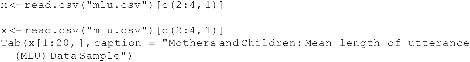
Mothers and Children: Mean Length of Utterance Data Sample

Group	Actor	Partner	Mean length of utterance
1	1M1	1C1	4.69
1	1M2	1C1	4.06
1	1C1	1M1	2.87
1	1C2	1M1	3.14
1	1M2	1C2	4.40
1	1M1	1C2	4.46
1	1C2	1M2	2.91
1	1C1	1M1	2.66
2	2M1	2C1	6.51
2	2M2	2C1	5.34
2	2C1	2M1	2.03
2	2C2	2M1	2.36
2	2M2	2C2	4.11
2	2M1	2C2	6.36
2	2C2	2M2	2.26
2	2C1	2M1	3.27
3	3M1	3C1	5.15
3	3M2	3C1	4.10
3	3C1	3M1	2.95
3	3C2	3M1	2.42

Next, we show the contrast coding, dummy, and ID codes required for the asymmetric block design and the glmmTMB call. In this data set, the choice of optimizer made a big difference in the estimates, suggesting that this data set may be too small for stable estimation. However, the substantive conclusions did not change (e.g., the mother’s partner effect is insignificant). In the glmmTMB call reported here, we use the default optimizer:

The fixed effects

The fixed-effects results are presented in Table 21. The intercept shows that children’s MLU is about 4, whereas mothers’ MLU, not surprisingly, is higher by about 2 units, and that difference is significant. Conversations between mothers and their own children have higher MLUs than conversations between mothers and other children, albeit this effect is insignificant, and it does not interact with the social category:

tabulateSRM.fixed(fit6, caption = "Fixed Effects")

Table 21.

Fixed Effects

		95% confidence interval
Variable	Estimate	Lower bound	Upper bound	p
(Intercept)	3.91	3.67	4.16	< .001
MCvCM	2.02	1.66	2.37	< .001
sameFamily	0.16	−0.03	0.36	.107
MCvCM:sameFamily	0.02	−0.22	0.27	.847

The random effects

The tabulateSRM.rand.uni has two arguments not shown yet. First, it allows one to change the default categories of men and women to mother and child. Second, it allows the addition of group variance to the table. The random-effects results are presented in Table 22. The random effects show substantial differences in actor effects between mothers and children. The actor variance of children accounts for the lion’s share of their total variance, 84.5%, whereas for mothers, it accounts for only about half of the variance. This reflects the difference in language use of toddlers versus adults. Adults appear to accommodate their language use to the two children (their own and the other), whereas toddlers do not. Further evidence for toddlers’ lack of MLU differentiation in response to different adults is the nonsignificant variance of mother’s partner effects. The lower confidence interval in this table is 0. Thus, different mothers do not elicit different MLU from different children:

Table 22.

Random Effects

			95% confidence interval
Component	Symbol	Estimate	Lower bound	Upper bound	Standardized
Mother
Group variance	${\mathrm{\sigma }}_{\mathrm{\mu }A}^2$	0.05	0.00	5.40	8%
Actor variance	${\mathrm{\sigma }}_{\mathrm{\alpha }A}^2$	0.28	0.10	0.77	41.6%
Partner variance	${\mathrm{\sigma }}_{\mathrm{\beta }B}^2$	0.06	0.01	0.72	9.2%
Relationship + error variance	${\mathrm{\sigma }}_{\mathrm{\gamma }A}^2$	0.28	0.14	0.54	41.2%
Actor–partner correlation	${\mathrm{\sigma }}_{\mathrm{\alpha }\mathrm{\beta }A}$	−.59	−.99	.97
Child
Group variance	${\mathrm{\sigma }}_{\mathrm{\mu }B}^2$	0.00	0.00	3724.77	0.3%
Actor variance	${\mathrm{\sigma }}_{\mathrm{\alpha }B}^2$	0.71	0.41	1.22	84.4%
Partner variance	${\mathrm{\sigma }}_{\mathrm{\beta }A}^2$	0.01	0.00	25.50	0.9%
Relationship + error variance	${\mathrm{\sigma }}_{\mathrm{\gamma }B}^2$	0.12	0.05	0.29	14.4%
Actor–partner correlation	${\mathrm{\sigma }}_{\mathrm{\alpha }\mathrm{\beta }B}$	.85	−.98	.99
Relationship correlation	${\mathrm{\sigma }}_{\mathrm{\gamma }\mathrm{\gamma }}$	.63	−.25	.88
Correlation between group means of mother and group means of child	${\mathrm{\sigma }}_{\mathrm{\mu }\mathrm{\mu }}$	.77	−1.00	1.00

Three variances in Table 22 have confidence intervals with a lower bound at zero: both the mothers’ and children’s group variances and the mothers’ partner effect. Therefore, we removed each of them in two steps. In addition, we removed the child’s partner effect to demonstrate that although it is small (9.2%), it could be significant. As the anova results below indicate, removing the group variances and their covariance, fit6alt1, did not affect the model’s fit, p = .98. Removing the mother’s partner effect, fit6alt2, had a negligible effect on the fit, p = .91. Note that the test of removing the mother’s partner has 2 df, one for the partner effect and one for the actor–partner correlations. Last, we dropped the child’s partner effect, fit6alt3, and found that removing it (Table 23) worsened the fit marginally, p = .06, suggesting that it could be a real effect had we had a larger sample. This raises the question of estimating power of SRM analyses, including the asymmetric block design (Lashley & Kenny, 1998). Lashley and Kenny (1998) showed in a simulation of SRM power that it increases more by increasing the number of participants in each group (in our case, the minimal four people with two mothers and two children) than by increasing the number of groups. For example, when partner variance in the population is 30%, the power of asymmetric block design with four participants is below 50%, and when there are 12 participants, the power is 100%. Thus, researchers planning to use SRM should attempt to create large groups rather than collecting data from more groups (assumed to be sampled from the same population):

Table 23.

Model Comparison: Removing the Mother’s Partner Variance and Actor–Partner Correlation Simultaneously

Model	df	Deviance		df	p
fit6alt3	9	260,835,381
fit6alt2	11	260,835,375	5.59	2	.06
fit6alt1	13	260,835,375	0.18	2	.91
fit6	16	260,835,375	0.17	3	.98

Discussion and Conclusion

We provide R codes for computing SRM components for data from asymmetric block designs, which are often used to study speed dating and other interactions of people from two social categories. We show how to use the glmmTMB and brms packages to estimate SRM parameters for three types of dependent variables: (a) one continuous variable, (b) multiple measures of a continuous variable, and (c) one dichotomous variable. We also show how to test additional predictors, such as the group effects and the order of interacting with others. Moreover, we discuss how to calculate correlations between SRM components of two variables: the actor–actor, partner–partner, partner–actor, actor–partner, intrapersonal dyadic, and interpersonal dyadic effects. We hope that these codes can be used to improve both transparency and reproducibility of psychology research of data collected with asymmetric block design and help a novice master the SRM analyses afforded by this design.

Supplemental Material

sj-pdf-1-amp-10.1177_25152459241279522 – Supplemental material for The Social-Relations Model for Asymmetric-Block-Design Data: A Tutorial With R

Supplemental material, sj-pdf-1-amp-10.1177_25152459241279522 for The Social-Relations Model for Asymmetric-Block-Design Data: A Tutorial With R by Avraham N. Kluger, Robert A. Ackerman, David A. Kenny, Thomas E. Malloy and Paul W. Eastwick in Advances in Methods and Practices in Psychological Science