Sage Journals: Discover world-class research

Abstract

Experience-sampling-method (ESM) studies have become a very popular tool to gain insight into the dynamics of psychological processes. Although the statistical modeling of ESM data has been widely studied, the preprocessing steps that precede such modeling have received relatively limited attention despite being a challenging phase. At the same time, adequate preprocessing of ESM data is crucial: It provides valuable information about the quality of the data and, importantly, helps to resolve issues in the data that may compromise the validity of statistical analyses. To support researchers in properly preprocessing ESM data, we have developed a step-by-step framework, a tutorial website that provides a gallery of R code, an R package, and templates to report the preprocessing steps. Particular attention is given to three different aspects in preprocessing: checking adherence to the study design (e.g., whether the momentary questionnaires were delivered according to the sampling scheme), examining participants’ response behaviors (e.g., compliance, careless responding), and describing and visualizing the data (e.g., examining distributions of variables).

Keywords

data preprocessing data preparation data quality experience-sampling method open badges open materials

The increasing interest in investigating the dynamics of within-persons psychological processes has made ambulatory assessment methods, such as the experience-sampling method (ESM) or ecological momentary assessment (EMA), an essential part of researchers’ toolkit (Trull & Ebner-Priemer, 2020; Van Roekel et al., 2019; Wrzus & Neubauer, 2022). ESM is a self-report method in which participants repeatedly complete a questionnaire about their everyday experiences, moods, symptoms, and contexts once or several times a day over a number of days (Myin-Germeys & Kuppens, 2022). The popularity of ESM can partly be explained by the wide variety of research questions that it allows to examine. To give some examples, researchers have investigated within-persons affective processes and how they are affected by daily events and person-level characteristics (Cloos et al., 2023), whether an impending relapse into depression can be foreseen (Schreuder et al., 2024; Snippe et al., 2023), the implementation and consequences of momentary interventions (Myin-Germeys et al., 2016), and whether romantic partners are in sync (Sels et al., 2020). Another crucial reason for its popularity is that participants are providing data in the real world. In contrast to experimental studies that focus on specific aspects of experience or behavior using controlled settings, ESM zooms into the flow of daily life experiences and thus into complex and uncontrollable but ecologically valid settings.

Because of this vast range of potential research questions, implementing ESM designs is challenging and involves a myriad of decisions (Heron et al., 2017; Janssens et al., 2018; Myin-Germeys & Kuppens, 2022). Among others, researchers have to decide on the type of sampling scheme (e.g., event-contingent, time-contingent), the sampling frequency (i.e., the number of measurement occasions within a day, which may differ across the items included), the type of items (e.g., Likert scales, sliders, categorical lists), and the response window (which may range from a few minutes to hours). Moreover, whereas most ESM studies focus on within-persons processes, some investigate interpersonal processes, implying that data are collected from dyads (e.g., romantic couples, mother-child, or even triads). This implies that the measurements of the members (e.g., romantic partners, family members) have to be aligned properly in that members are sent momentary questionnaires at the same time or in sequential order. After designing the momentary questionnaires and the sampling scheme for each item, researchers have to choose software to handle the data collection. Given the popularity of ESM research, multiple packages and apps have been developed (see J. D. M. Weermeijer, Kiekens, & Wampers, 2022), such as m-Path (Mestdagh et al., 2023), SEMA3 (O’Brien et al., 2023), or formr (Arslan et al., 2020; Blanchard et al., 2023). Each software obviously comes with its own particularities when collecting, storing, and exporting data. Another important consideration is that ESM studies can be burdensome to participants. Participants may therefore sometimes accidentally or intentionally miss measurement occasions or adopt careless response styles (Eisele et al., 2022, 2023; Rintala et al., 2019).

Hence, a rigorous quality investigation after data have been collected is crucial. This involves steps such as checking whether the design choices were correctly implemented and whether the participants were compliant. For example, researchers should verify whether the total number of beeps and the frequency with which they were sent to each participant align with what was initially planned. Moreover, if researchers allowed only a limited amount of time to respond to momentary questionnaires, it should be checked whether responses indeed fall within this response window and how many momentary responses are missing. Beyond checking and solving issues in the data, researchers may also need to compute variables of interest, prepare the data for analysis, and obtain descriptive statistics and visualizations that can provide insights into relevant data patterns (e.g., distribution shapes; Viechtbauer, 2021).

Going through these checking, preparing, and descriptive-statistics steps is challenging. Researchers usually come up with their own preprocessing pipeline because of a lack of available tools, frameworks, and templates to preprocess ESM data (e.g., Miché, 2019; Viechtbauer, 2021; Viechtbauer & Constantin, 2023). In addition, the preprocessing steps taken are often not reported in a transparent manner. The latter is critical for reproducibility, especially given the variability in preprocessing steps and their potential effect on the results of further statistical analyses. Moreover, documenting the preprocessing steps also improves collaboration efficiency (e.g., common understanding of the database) and reusability of the data.

We therefore propose a step-by-step ESM preprocessing framework. We further assist researchers in developing code to preprocess their ESM data by providing a website with tutorials and an R-code gallery and an associated R package called, respectively, the “ESM preprocessing gallery” (https://preprocess.esmtools.com/) and the “esmtools R package” (https://package.esmtools.com). Finally, we provide Rmarkdown templates to support researchers in documenting and sharing their preprocessing pipeline.

In the following sections of this article, we introduce the framework, website, R package, and reporting templates, starting from an illustrative data set. Then, in a dedicated tutorial section, we demonstrate how they can be used to conduct specific preprocessing tasks for the illustrative data.

Method

Illustrative Data Set

Study design

We consider data from a pilot ESM study in which 10 families (triads of father–mother–child) participated. In this study, researchers wanted to investigate covariation between family members’ positive and negative affect and (in)congruencies in their perception of stressful events experienced by the child. Family members received a notification (beep) prompting them to complete a questionnaire four times a day on weekdays (between 4:30 p.m. and 8:30 p.m.) and nine times a day on weekend days (between 10:15 a.m. and 8:30 p.m.) for 10 consecutive days, yielding 60 beeps in total. Beeps were sent semirandomly within predetermined 15-min time intervals, with the restriction that there was always at least 1 hr between two consecutive beeps. The beeps were sent at the same time to family members and expired after 30 min.

In this article, we use only a part of the data set, that is, we focus on the father-mother dyads, excluding the children’s data, and examine a subset of the assessed variables.¹ We examine parents’ momentary positive affect and negative affect (rated on scales ranging from 0 to 100). In addition, identification variables (i.e., participant number, dyad number), demographic variables (i.e., “role” (father/mother), “age”), and timestamp variables “scheduled” (i.e., when the ESM questionnaire was scheduled), “sent”’ (i.e., when the questionnaire was sent), “start” (i.e., when the questionnaire was opened by the participant), and “end” (i.e., when the questionnaire was completed) were retained. Table 1 displays a subset of rows.² This raw data set is stored in the esmtools R package and imported in the actual R session (“esmdata_raw” variable) whenever the esmtools package is loaded (see Code Snippet 3 in the Appendix).

Table 1.

Subset of Rows From the Illustrative Data Set

dyad	id	role	age	scheduled	sent	start	end	pos_aff	neg_aff
1	13	1	44	2022-05-06 16:37:09	2022-05-06 16:37:11	2022-05-06 16:37:29	2022-05-06 16:41:08	96	4
1	13	1	44	2022-05-06 17:50:02	2022-05-06 17:50:03	2022-05-06 17:50:25	2022-05-06 17:53:26	89	0
1	13	1	44	2022-05-06 19:09:55	2022-05-06 19:09:57	2022-05-06 19:14:16	2022-05-06 19:17:00	94	0
1	13	1	44	2022-05-06 20:19:37	2022-05-06 20:19:38	2022-05-06 20:19:52	2022-05-06 20:22:22	97	4
1	13	1	44	2022-05-07 10:25:22	2022-05-07 10:25:24	2022-05-07 10:26:01	2022-05-07 10:28:32	91	8
1	13	1	44	2022-05-07 11:36:59	2022-05-07 11:37:00	2022-05-07 11:37:56	2022-05-07 11:40:23	85	0

Preprocessing tasks

When preprocessing our illustrative data set, many aspects should be checked that can be divided into five preprocessing steps (see Table 2 and description of the framework below). Here, we describe a representative example per step, which we use later in the tutorial section.

Table 2.

Topics Available in the ESM Preprocessing Gallery Website That Are Attached to Each Step of the ESM Preprocessing Gallery

	Steps	Main task	Composition
1	Import data and preliminary preprocessing	Import data, first insight on variables and data structure, basic preprocessing and checking variable consistency	• Import data and merge data sources
			• First glimpse of the data
			• Check data structure and reformat (e.g., long format)
			• Rename and relabel variables
			• Reformat variables
			• Check duplication (e.g., rows, timestamps, pattern of answers)
			• Check variables’ type-values coherence
			• Check branching items
			• Create time variables (e.g., observation number)
			• First missing values analysis
			• Define and flag (in)valid observations
2	Design and sampling scheme	Investigate the adherence of the data collection to the predefined sampling scheme and study design	• Calendar plot
			• Sampling scheme plot
			• Time beeps were sent
			• Participant’s involvement duration
			• Quantity of beeps sent
			• Delay to send beeps
			• Delay between consecutive sent beeps
			• Check timestamps coherence
			• Dyadic delay in sending
3	Participants’ response behaviors	Investigate participants’ response behaviors and the extent to which they adhered to the sampling scheme and study design	• Sampling scheme of participants’ answers
			• Time the beeps were started or missed
			• Delay to start and to answer
			• Delay between consecutive answers
			• Response rates (e.g., number of valid answers in time)
			• Number of interactions with the items
			• Correlates of missed beeps
			• Careless responses (i.e., longstring, response time)
			• Compliance rate
4	Compute and transform variables	Compute and modify variables of interests	• Compute common scores (e.g., mean, standard deviation)
			• Lag and center variables
			• Check computation procedure
			• Compute common affect scores
5	Descriptive statistics and visualization	Descriptive insights on the variables and both within-processes dynamics and between-participants differences	• Summary tables (e.g., descriptive statistics)
			• Distributions plots
			• Distributions of participant statistics
			• Time-series visualization
			• Correlation plots
			• Autocorrelation and cross-correlation plots

First, we must confirm that variables are consistent with their type. For instance, the identification variables (i.e., participant and dyad identifier) and demographic variables (i.e., role, age) should be time-invariant and thus display only one value per participant (Illustration 1). Second, we can check whether the sampling scheme was properly followed during data collection. In particular, did the participant receive the correct number of beeps on weekdays and weekend days (Illustration 2)? Third, we examine participants’ response behaviors and might want to know how much time participants took to answer each beep and check for outliers therein (Illustration 3). Fourth, to prepare the data for statistical analysis, specific preprocessing steps have to be taken. Among them, we want to person-mean center positive and negative affect (Illustration 4) to later use them as predictors in a statistical model (Enders & Tofighi, 2007). Finally, we can be interested in knowing the distribution of the variable at a participant level, that is, whether it follows a normal, skewed, or bimodal distribution (Illustration 5). Illustrations 1 to 3 are used below in the tutorial section, and Illustrations 4 and 5 are discussed in the supplementary materials available on the repository website (https://gitlab.kuleuven.be/ppw-okpiv/researchers/u0148925/esm_preprocessing_gallery/-/tree/master/docs/Supplementary_illustrations.pdf).

ESM preprocessing framework, R-code website, R package, and reporting

Description of the framework

The ESM preprocessing framework (see Fig. 1 and Table 2) is thus composed of five steps. The first three steps and the final one are relatively independent of the specific study at hand, whereas Step 4 depends more strongly on the research question being addressed.

Fig. 1.

Five steps of the experience-sampling-method preprocessing framework.

Step 1: import data and preliminary preprocessing

First, tasks in this step include importing the data set(s) and, if applicable, merging the different data sources. Importing data can be a challenging task in itself because data may be stored in various formats (e.g., .csv, .sav) and may be split up across different files, such as separate files per day or per participant. Next, one must perform some basic activities, such as checking for duplicated observations, relabeling and renaming variables, and gaining an overview of the variables and the data-set structure. An ESM study includes different variable types, such as subject-identifier variables (e.g., participant numbers), time-varying variables (e.g., positive/negative affect), and time-invariant variables (e.g., demographics, personality traits). Each variable in the data set comes with a specific set of expectations regarding its properties and values, necessitating thorough verification to ensure data quality. For instance, identification variables must not include missing values and must have a different number for each participant and/or dyad. Variable values must consistently fall within the specified response range (e.g., 0–100 for sliders). Temporal variables, such as timestamps, must exhibit chronological consistency, with timestamps occurring in the expected order. Finally, we note that when merging data sources, often some preliminary preprocessing tasks (e.g., relabeling variables, adding participant IDs) need to be completed before merging.

Step 2: design and sampling scheme

This step entails evaluating the adherence of the data collection to the predefined sampling scheme and study design. ESM studies typically employ predetermined designs and sampling schemes, but issues can cause the collected data set to deviate from its intended trajectory. Issues can stem from recording, server, and database storage issues, or they can be human-related. For instance, a phone in airplane mode might miss questionnaires, or there might be problems with timestamp recordings or sampling-scheme programming. Investigating “scheduled” (i.e., the time the questionnaire was planned) and “sent” (i.e., the time the questionnaire was sent to the participant) timestamp variables can provide valuable information in this regard.

Step 3: participants’ response behaviors

This step entails investigating participants’ response behaviors and the extent to which they adhered to the sampling scheme and study design. For instance, what are participants’ response times to start and complete questionnaires? Are responses to beeps missing, and is this missingness related to the time of the day? In the literature, three principal aspects often investigated are the compliance rates³ (Hasselhorn et al., 2021; Rintala et al., 2019; Wen et al., 2017; Wrzus & Neubauer, 2022), careless responding⁴ (Curran, 2016; Denison & Wiernik, 2020; Eisele et al., 2022; Meade & Craig, 2012), and the delay of response⁵ (Boukhechba et al., 2018; Eisele et al., 2021). Next to these, additional patterns of response behaviors and missing values can be investigated, such as whether noncompliance or careless responses are related to time-invariant (e.g., age) or moment-level (e.g., time of the day) variables (e.g., Rintala et al., 2020).

Step 4: compute and transform variables

In Step 4, we calculate and modify variables of interest. These modifications must be in line with the research question and the planned analysis. For instance, in psychological research, it is common to use a group of items to capture a specific construct. Hence, items are often aggregated into a construct score, such as by calculating means or sums. In addition, specific analyses might require variables to be transformed in a specific way. For instance, researchers who investigate predictive relations over time by using autoregressive modeling will have to lag variables. If multilevel approaches are used, then person-mean centering time-varying variables may be necessary. Computing these scores can occasionally pose challenges because the nested structure of ESM data has to be taken into account as well as the ordering of the observations.

Step 5: descriptive statistics and visualization

In this step, we compute descriptive statistics and visualize the data to gain insight into the variables of interest and the within-persons processes. For example, we can examine variables’ distributions to better understand if there are, for instance, floor effects, multimodality, or skewness. We also get insight into whether the variables’ distributions are dependent on a group variable or the occurrence of an event. In addition, we can visualize variable scores across time to shed light on within-processes dynamics and between-participants differences therein. For instance, we can investigate individuals’ time series to check for potential trends or seasonal patterns.

R-code website and R package

The ESM preprocessing gallery (see Fig. 2) is a website (https://preprocess.esmtools.com) that includes a set of specific topics for each of the five steps of the ESM preprocessing framework. To access a topic of interest, users need to click on the relevant icon on the home page (e.g., click on “Delay two answered beeps” under “Step 3” to examine the time distribution between two answered beeps for each participant). For each topic, comprehensive instructions are provided, accompanied by R code and application examples. Users can then copy-paste the relevant R code and tailor it to their specific data set and needs. Examples of the topics are built on (parts of) a synthetic data set (for details, see https://preprocess.esmtools.com/terminology.html). Note that this synthetic data set is not the data set used in this article. The data set is made specific for each topic and can be downloaded at the top of each topic’s page by clicking on the button “Download data.”

Fig. 2.

Screenshot of the index page of the experience-sampling method preprocessing gallery website.

The ESM preprocessing gallery is accompanied by an R package, the esmtools package (https://package.esmtools.com), which is available on CRAN and can be downloaded (see Code Snippet 1 in the Appendix).

Templates

To support researchers in sharing and documenting their preprocessing pipeline, we also provide Rmarkdown templates (Allaire et al., 2024). We developed a first example template to report on the preprocessing phase and another example template to report on the characteristics of the preprocessed data set. These templates serve as support, and their structures and organizations can be adapted (e.g., preprocessing different data sources before merging them) to correspond to specific needs. In-depth explanations can be found on the website in the “Preprocessing report” and “Data characteristics report” sections of the website and the Rmarkdown files and associated HTML files for our illustrative data (https://gitlab.kuleuven.be/ppw-okpiv/researchers/u0148925/esm_preprocessing_gallery/-/tree/master/report_examples).

Preprocessing report

The preprocessing report (see https://preprocess.esmtools.com/pages/90_Preprocessing_report.html) describes Steps 1 to 5, the packages loaded, which data are imported, and how the preprocessed data are exported. In brief, it helps to document and share “what has been done and checked” in the raw data set to get the preprocessed one (for an example, see https://preprocess.esmtools.com/report_examples/Preprocessing_report_advanced_example.html). The report should ideally report all analyses that have been performed. Particular emphasis should be placed on the issues that were spotted and data transformations done (e.g., removing observations and participants) along with their motivations (e.g., observation belonging to a piloting phase). For that purpose, users can use the “txt()” function from the esmtools package (see https://preprocess.esmtools.com/pages/90_Reporting_tools.html). For additional support, two template versions following the same structure are available through the esmtools package, “preprocess_report” and “advanced_preprocess_report,” and can be imported using the “use_template()” function in an R terminal (Code Snippet 2 in the Appendix). The difference between the two templates pertains to additional tools. The advanced template goes with additional functions that may help improve the readability of the report (e.g., collapsing buttons, highlighting specific elements such as errors, data-set tracking). These functions are especially helpful when the preprocessing report is long because readers can otherwise get lost and not get the essential information. Because preprocessing ESM data can be challenging, we provide a list of minimal checks to perform (see https://preprocess.esmtools.com/preproc_list.html). However, it should be regarded as a starting point rather than a definitive guide.

Data characteristics report

The data characteristics report (https://preprocess.esmtools.com/pages/90_Data_characteristics_report.html) includes a series of descriptive analyses to efficiently share “what the preprocessed data looks like” and get in-depth insights into its characteristics and qualities (for an example, see https://preprocess.esmtools.com/report_examples/Data_characteristics_report_example.html). This report is crucial for gaining a comprehensive understanding of the data set before applying any statistical models and for acquiring knowledge about the phenomenon under investigation and the variables collected (Siepe et al., 2024; Viechtbauer, 2021). In addition, it simplifies data sharing by offering comprehensive descriptive statistics and serves as an additional check to ensure that no errors have been overlooked or even introduced during the data-preprocessing stage. For instance, the incorrect application of a threshold to exclude careless responses (in Step 3) can add extra missing values in variables that were previously checked and validated in earlier steps (e.g., timestamp variables in Step 2). Note that this report differs from the preprocessing one by using descriptive statistics and visualizations on the fully preprocessed data set rather than the raw data set.

The data-characteristics report consists of three parts. First, it includes a broad description of each variable. Second, it includes a user’s selection of descriptive statistics and visualizations from Steps 1 to 4. These are important to understand the quality of participants’ response behaviors and to get insight into how well the data-collection procedure has been done (including data-collection issues that could not be solved). Third, any descriptive statistic from Step 5 can be included that would be relevant for present or future studies. We strongly recommend that researchers document the characteristics of the collected items and their aggregated scores, for instance, their distributions within participants and the investigation of temporal factors (e.g., differences between weekdays and weekend days). This last section can also include a participant book. A participant book contains descriptive statistics and visualization of relevant participants’ response behaviors and variables of interest in a table, with one row for each participant. The data-characteristics-report template is stored in the esmtools package and can be imported using “esmtools::use_template(‘data_characteristics_report’, output_dir = getwd()).”

The preprocessing report and the data-characteristics reports hold information that overall benefits the transparency and the reproducibility of a study. Such information would also benefit the preregistration of secondary data analyses because it supports choosing suitable statistical models and prevents postpreregistration deviations (Kirtley et al., 2021). Nonetheless, it is essential to exercise caution in this process. In the context of a research project, the information contained in reports should be accessed only after the research questions have been clearly defined and operationalized to prevent research malpractices, such as confirmation bias (Begley & Ioannidis, 2015; Mynatt et al., 1977).

Tutorial

In this section, we present a tutorial on how to use our tools to address the first three preprocessing questions raised for our illustrative data; tutorials for Questions 4 and 5 are provided in the supplemtary material. In each illustration, we also demonstrate the integration of the code into a preprocessing report, with texts highlighting the identified issues and the data transformations made. The text is highlighted using the “txt()” function from the esmtools package (see https://preprocess.esmtools.com/pages/90_Reporting_tools.html). The full code is displayed in the Appendix of this article (see Code Snippet 12 in the Appendix). Note that the five illustrations presented do not check every relevant aspect of the illustrative data set. The complete preprocessing report of this data set is provided as an example on the website (see https://preprocess.esmtools.com/report_examples/Preprocessing_report_advanced_example.html).

Before introducing the illustrations, we first create a new RMarkdown document⁶ and load the packages that will be used in the illustrations: dplyr (data management; Wickham et al., 2023), ggplot2 (data visualization; Wickham, 2016), lubridate (handling date and time; Grolemund & Wickham, 2011), and the esmtools package. Then, as part of Step 1, we import the raw data set stored in the esmtools R package (Code Snippet 3 in the Appendix). Finally, timestamp variables need to be reformatted into a POSIXct format. On the website, tips and good practices are provided in the “Reformatting” topic (https://preprocess.esmtools.com/pages/40_Reformatting.html). In this topic, we see that by using a combination of “the mutate()” and “across()” functions, we can reformat multiple variables at once (Code Snippet 4 in the Appendix). We copy and paste the code and proceed to the adaptations. We replace the variables “PA1,” “PA2,” and “PA3” with the timestamp variables “scheduled,” “sent,” “start,” and “end.” We also change the “as.numeric” by the “as.POSIXct” function. Figure 3 shows the integration of the code and an associated descriptive text to highlight the data transformation made.

Fig. 3.

Incorporating reformatting of the timestamp variables into POSIXct format.

Illustration 1: check coherence of time-invariant variables

One characteristic of time-invariant variables, such as demographic variables, is to display only one unique value per participant. Here, as part of Step 1 of the ESM preprocessing framework, our specific aim is to check if the age variable takes more than one value or a missing value per participant. For instance, in Figure 1, Participant 13 is age 44 years. This means that throughout the observations, only this age value should be assigned to this participant. To check if this is indeed the case, we go to the “Check variable coherence” topic of the website (https://preprocess.esmtools.com/pages/40_Check_variable_coherence.html). There, we have a subpart called “Check if variables are time-invariant for each subject,” which provides three methods to perform this task. We opt for the final one, which uses a function from the esmtools package.

Hence, we copy and paste the function in the Step 1 section of our preprocessing template. To make the function work for our specific task and data, we specify the function’s arguments by indicating the data frame (“data”) and the time-invariant variables we want to check (“age”).⁷ In addition, because the purpose here is to check at the participant level, we indicate the “id” variable as the grouping variable⁸ (Code Snippet 5 in the Appendix). After running the code, we see in the output that the participants with the “id” 32 and 46 have two age values each, (47, 29) and (49, 22), respectively. Figure 4 shows the integration of the code, its output, and an associated descriptive text to highlight the issue. We recommend investigating those participants’ observations (or in the case of dyadic data, also observations of the partner) before coming to a decision about how to solve this issue.

Fig. 4.

Incorporating variable consistency checks using the “vars_consist()” function.

Illustration 2: check sampling scheme

As part of Step 2, we want to check whether the actual sampling scheme of each participant is in line with the predefined one. In our study, this means that we want to know if participants received four beeps each weekday and nine beeps each weekend day, if data-collection days are consecutive, and if piloting observations are already removed from the database. We go to check the “Sampling scheme plot” topic on the website (https://preprocess.esmtools.com/pages/50_Sampling_scheme_plot.html) and rely on the “Day level” subsection. Its output gives a sampling plot that displays for each participant (y-axis) the number of beeps sent (color code) per day involved in a study (x-axis). We also follow a recommendation in the “Integrate other information” subsection to integrate the type of day information (weekday vs. weekend day) in the plot.

This plot requires computing two time-related variables: the “daycum” (i.e., day number since the first beep sent to the participant) and “weekday” variables (i.e., indicates if the beep belongs to a weekday or a weekend day). Instruction about how to compute those variables can be found in the “Create time variables” topic (https://preprocess.esmtools.com/pages/40_Create_time_variables.html) in the subsection “Cumulative day” (Code Snippet 6 in the Appendix) and “Weekday vs. weekend day” (Code Snippet 7 in the Appendix). The codes do not need modifications because the variable names are identical to those in our data set. Figure 5 shows the integration of the code and the description of the data transformation made.

Fig. 5.

Incorporating creation of the “weekday” and the “daycum” variables.

We further adapted the code of the plot found on the website to our specific task and data. We first integrated the “weekday” to the grouping function with the “id” and “daycum” variables (“group_by()”). In addition, we use different shapes to represent week versus weekend days (“geom_point(aes(. . ., shape=weekday), . . .)”), rotate the x-axis label to 90° (“theme(axis.text.x = element_text(angle = 90))”), and add new titles to the axis and the plot (Code Snippet 8 in the Appendix). In the output, we see the expected variations between weekdays and weekends in terms of the number of beeps sent. However, it also reveals unexpected patterns. The initial day of the study typically consists of a single observation and is for several participants followed by a number of days without beeps. Figure 6 shows the integration of the code, the output, and the description of the issues found.

Fig. 6.

Incorporating and adapting the sampling-scheme plot. Identified issues are highlighted at the top. The figure illustrates the daily count (x-axis) of sent beeps (color-coded legend) for each participant (y-axis), distinguishing between weekday and weekend days (shape-coded legend).

Illustration 3: time needed to fill the questionnaire

As part of Step 3 of the ESM preprocessing framework, we want to investigate the within- and between-participants variability in the time participants took to answer each valid beep and see if there are any outliers that need further investigation. To get a plot of this information, we check the “Delay to start and to fill” topic on the website (https://preprocess.esmtools.com/pages/60_Delay_to_start_and_to_fill.html). To particularly investigate the distribution, we want to create box plots that display the delay distributions of each participant. To do so, we use the code of the plot presented in the “Grouping-variables” subsection. The plot displays a combination of scatterplots and boxplots, with the time to fill the questionnaires on the x-axis and the different participants on the y-axis. This plot is particularly helpful in highlighting within- and between-persons differences in response delays and outliers. This plot requires the creation of two additional variables not already included in the data set.

We first have to compute the “delay_end_min” variable at the start of the topic. Created using the “difftime()” function, this variable contains the delay in minutes computed as the difference between the start variable and the end variable (Code Snippet 9 in the Appendix). Fortunately, this code does not need modifications to be integrated because variable names are identical in our data set and the unit specified is already minutes. Figure 7 shows the integration of the code and an associated descriptive text to highlight the data transformation made.

Fig. 7.

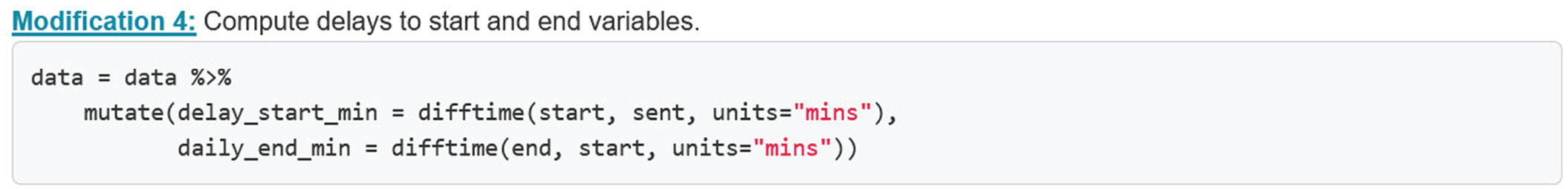
Incorporating the creation of the “delay_start_min” and the “delay_end_min” variables.

Because we want to investigate only the delay for valid beeps, we first have to define when the observations at specific beeps will be considered valid and flag the observations accordingly (1 = valid, 0 = invalid) and store the result in the “valid” variable (for further information, see the “Flag (in)valid observation” topic on the website). Note that in the preprocessing workflow, it is recommended to compute this variable at the end of Step 1. This approach allows us to easily flag invalid observations because they can be revealed at later steps. In our illustration, we considered an observation to be valid whenever the variables of interest (i.e., “pos_aff,” “neg_aff,” and “perc_fun_signaled”) are not missing. A set of logical tests can be used to create the “valid” variable (Code Snippet 10 in the Appendix). Figure 8 shows the integration of the code and an associated descriptive text to highlight the data transformation made.

Fig. 8.

Incorporating the creation of the “valid” variable.

Going back to the creation of the plot, we made minor code modifications, including adding labels to the axis and a title to the plot (Code Snippet 11 in the Appendix). The resulting plot gives a lot of information. For instance, we see that there is no response-time interval close to or below 0 min and that Participants 20, 52, 72, and 80 took less time on average. We also see Participants 49, 67, 73, and 77 show more variability in the time interval to fill, and Participants 7, 66, 73, 77, and 15 display some outliers (>5 min and even >10 min for Participant 15). Figure 9 shows the integration of the code, its output, and highlighted issues. Further investigations are required to address and resolve these potential issues.

Fig. 9.

Incorporating and adapting the code to create a plot about the delay in filling the surveys. The identified issues are highlighted at the top. The figure contains one box plot per participant (y-axis) of the delay to fill the surveys (x-axis).

Discussion

Developing a clear and reproducible preprocessing report when preprocessing ESM data is an important step toward more transparent and reproducible ESM studies. We hope and expect that our proposed tools will enhance the ease and thoroughness of preprocessing ESM data and will encourage researchers to report on the steps taken.

The toolbox raises important questions for future research. First, our tools are only a first building block rather than an exhaustive compendium. Indeed, preprocessing ESM data is challenging, takes many forms, and might be very specific to the data or the study design at hand. Note that the tools developed here do not address every aspect. For example, preprocessing a dyadic data set often involves additional data checking to ensure that each row contains responses from Partner A and Partner B at each beep (Lafit et al., 2022). Mobile sensing can also imply handling extra preprocessing challenges to combine both the sensing and the ESM data (De Calheiros Velozo et al., 2024). Looking ahead, innovative designs could drastically change the way researchers need to preprocess their data. Hence, we made this project collaboration-friendly and warmly invite researchers to improve and extend the esmtools R package and the ESM preprocessing gallery (https://preprocess.esmtools.com/about.html). This allows researchers to add topics about, for instance, specific methods to flag and handle careless responses or to import and restructure data collected using specific software.

Second, ESM studies offer a wealth of indicators that can be extracted to evaluate various aspects of data collection at both the software and participant levels. These indicators encompass how often the software failed to deliver beeps at the right time, at which times of the day participants are more likely to answer beeps, the delay to start a beep, the delay to end the survey, or specific indicators of careless responding (Geeraerts & Kuppens, 2020). Future studies could focus on how those indicators should be interpreted and how to understand their intra- and interindividual variance. In addition, their relevance for defining data quality can be explored because data quality is a quite complex construct (see Batini et al., 2009). A key consideration is to determine which of the many possible indicators yield the most useful information. A better understanding of data quality would not only be helpful in the analysis phase. Indeed, a key question for research on sample-size planning of ESM studies is how to integrate potential data-quality issues in the sample-size recommendations (Lafit et al., 2021).

Finally, much like data analysis (Kirtley et al., 2021; Silberzahn et al., 2018), preprocessing pipelines can be associated with forking paths. Different researchers working with the same data set may employ distinct preprocessing methods and may not check the same aspects of the data set or do so in a different way. Access to the precise preprocessing details of studies could encourage researchers to critically evaluate their own pipelines and adopt practices from different researchers. It could also facilitate investigations into preprocessing practices and their potential impact on study outcomes. For example, missingness mechanisms, temporal patterns of missings, and compliance levels may affect conclusions (see e.g., Simsa et al., 2024; J. Weermeijer, Lafit, et al., 2022). Thus, reporting on the preprocessing can contribute to the development of guidelines and tutorials tailored to various ESM study designs.

Footnotes

Appendix

Acknowledgements

We express our gratitude to Kristof Meers for his valuable technical inputs on both the R package and the websites.

Transparency

Action Editor: Pamela Davis-Kean

Editor: David A. Sbarra

Author Contributions

Jordan Revol: Conceptualization; Project administration; Software; Writing – original draft; Writing – review & editing.

Chiara Carlier: Software; Writing – review & editing.

Ginette Lafit: Conceptualization; Supervision; Writing – original draft; Writing – review & editing.

Martine Verhees: Data curation; Software; Writing – review & editing.

Laura Sels: Software; Writing – review & editing.

Eva Ceulemans: Conceptualization; Funding acquisition; Software; Supervision; Writing – original draft; Writing – review & editing.

ORCID IDs

Jordan Revol

Ginette Lafit

Notes

References

Allaire

Xie

Dervieux

McPherson

Luraschi

Ushey

Atkins

Wickham

Cheng

Chang

Iannone

(2024). Rmarkdown: Dynamic documents for R (R package Version 2.27) [Computer software]. Retrieved from https://github.com/rstudio/rmarkdown

Arslan

R. C.

Walther

M. P.

Tata

C. S.

(2020). Formr: A study framework allowing for automated feedback generation and complex longitudinal experience-sampling studies using R. Behavior Research Methods, 52(1), 376–387.

Batini

Cappiello

Francalanci

Maurino

(2009). Methodologies for data quality assessment and improvement. ACM Computing Surveys, 41(3), 1–52.

Begley

C. G.

Ioannidis

J. P.

(2015). Reproducibility in science: Improving the standard for basic and preclinical research. Circulation Research, 116(1), 116–126.

Blanchard

M. A.

Revol

Hoebeke

Roskam

Mikolajczak

Heeren

(2023). On the temporal nature of parental burnout: Development of an experience sampling methodology (ESM) tool to assess parental burnout and its related ever-changing family context. Collabra: Psychology, 9(1), Article 74614. https://doi.org/10.1525/collabra.74614

Boukhechba

Cai

Chow

P. I.

Fua

Gerber

M. S.

Teachman

B. A.

Barnes

L. E.

(2018). Contextual analysis to understand compliance with smartphone-based ecological momentary assessment. In Proceedings of the 12th EAI International Conference on Pervasive Computing Technologies for Healthcare (pp. 232–238). Association for Computing Machinery.

Cloos

Ceulemans

Kuppens

(2023). Development, validation, and comparison of self-report measures for positive and negative affect in intensive longitudinal research. Psychological Assessment, 35(3), 189–204.

Curran

P. G.

(2016). Methods for the detection of carelessly invalid responses in survey data. Journal of Experimental Social Psychology, 66, 4–19.

De Calheiros Velozo

Habets

George

S. V.

Niemeijer

Minaeva

Hagemann

Herff

Kuppens

Rintala

Vaessen

Riese

Delespaul

. (2024). Designing daily-life research combining experience sampling method with parallel data. Psychological Medicine, 54(1), 98–107. https://doi.org/10.1017/S0033291722002367

10.

Denison

A. J.

Wiernik

B. M.

(2020). Careless response processes are heterogeneous: Comment on Goldammer et al. (2020). PsyArXiv. https://doi.org/10.31234/osf.io/9rk4

11.

Eisele

Vachon

Lafit

Kuppens

Houben

Myin-Germeys

Viechtbauer

(2022). The effects of sampling frequency and questionnaire length on perceived burden, compliance, and careless responding in experience sampling data in a student population. Assessment, 29(2), 136–151.

12.

Eisele

Vachon

Lafit

Tuyaerts

Houben

Kuppens

Myin-Germeys

Viechtbauer

(2023). A mixed-method investigation into measurement reactivity to the experience sampling method: The role of sampling protocol and individual characteristics. Psychological Assessment, 35(1), 68–81.

13.

Eisele

Vachon

Myin-Germeys

Viechtbauer

(2021). Reported affect changes as a function of response delay: Findings from a pooled dataset of nine experience sampling studies. Frontiers in Psychology, 12, Article 580684. https://doi.org/10.3389/fpsyg.2021.580684

14.

Enders

C. K.

Tofighi

(2007). Centering predictor variables in cross-sectional multilevel models: A new look at an old issue. Psychological Methods, 12(2), 121–138.

15.

Geeraerts

Kuppens

(2020). Investigating careless responding detection techniques in experience sampling methods (ESM). KU Leuven.

16.

Grolemund

Wickham

(2011). Dates and times made easy with lubridate. Journal of Statistical Software, 40(3), 1–25.

17.

Hasselhorn

Ottenstein

Lischetzke

(2021). The effects of assessment intensity on participant burden, compliance, within-person variance, and within-person relationships in ambulatory assessment. Behavior Research Methods, 54(4), 1541–1558.

18.

Heron

K. E.

Everhart

R. S.

McHale

S. M.

Smyth

J. M.

(2017). Using mobile-technology-based ecological momentary assessment (EMA) methods with youth: A systematic review and recommendations. Journal of Pediatric Psychology, 42(10), 1087–1107.

19.

Janssens

K. A. M.

Bos

E. H.

Rosmalen

J. G. M.

Wichers

M. C.

Riese

(2018). A qualitative approach to guide choices for designing a diary study. BMC Medical Research Methodology, 18(1), Article 140. https://doi.org/10.1186/s12874-018-0579-6

20.

Kirtley

O. J.

Lafit

Achterhof

Hiekkaranta

A. P.

Myin-Germeys

(2021). Making the black box transparent: A template and tutorial for registration of studies using experience-sampling methods. Advances in Methods and Practices in Psychological Science, 4(1). https://doi.org/10.1177/2515245920924686

21.

Lafit

Adolf

J. K.

Dejonckheere

Myin-Germeys

Viechtbauer

Ceulemans

(2021). Selection of the number of participants in intensive longitudinal studies: A user-friendly shiny app and tutorial for performing power analysis in multilevel regression models that account for temporal dependencies. Advances in Methods and Practices in Psychological Science, 4(1). https://doi.org/10.1177/2515245920978738

22.

Lafit

Sels

Adolf

J. K.

Loeys

Ceulemans

(2022). PowerLAPIM: An application to conduct power analysis for linear and quadratic longitudinal actor–partner interdependence models in intensive longitudinal dyadic designs. Journal of Social and Personal Relationships, 39(10), 3085–3115. https://doi.org/10.1177/02654075221080128

23.

Meade

A. W.

Craig

S. B.

(2012). Identifying careless responses in survey data. Psychological Methods, 17(3), 437–455.

24.

Mestdagh

Verdonck

Piot

Niemeijer

Kilani

Tuerlinckx

Kuppens

Dejonckheere

(2023). M-Path: An easy-to-use and highly tailorable platform for ecological momentary assessment and intervention in behavioral research and clinical practice. Frontiers in Digital Health, 5, Article 1182175. https://doi.org/10.3389/fdgth.2023.1182175

25.

Miché

(2019). esmprep: Data preparation during and after the use of the experience sampling methodology (ESM) (R package Version 0.2.0) [Computer software]. Retrieved from https://CRAN.R-project.org/package=esmprep

26.

Myin-Germeys

Klippel

Steinhart

Reininghaus

(2016). Ecological momentary interventions in psychiatry. Current Opinion in Psychiatry, 29(4), 258–263.

27.

Myin-Germeys

Kuppens

(Eds.). (2022). The open handbook of experience sampling methodology: A step-by-step guide to designing, conducting, and analyzing ESM studies (2nd ed.). Center for Research on Experience Sampling and Ambulatory Methods Leuven.

28.

Mynatt

C. R.

Doherty

M. E.

Tweney

R. D.

(1977). Confirmation bias in a simulated research environment: An experimental study of scientific inference. Quarterly Journal of Experimental Psychology, 29(1), 85–95.

29.

O’Brien

S. T.

Hinton

J. D. X.

Moeck

Susanto

Jayaputera

Sinnott

R. O.

Alvarez-Jimenez

Gleeson

Koval

(2023). SEMA3: A free smartphone platform for daily life surveys. PsyArXiv. https://doi.org/10.31234/osf.io/cnar8

30.

Rintala

Wampers

Myin-Germeys

Viechtbauer

(2019). Response compliance and predictors thereof in studies using the experience sampling method. Psychological Assessment, 31(2), 226–235.

31.

Rintala

Wampers

Myin-Germeys

Viechtbauer

(2020). Momentary predictors of compliance in studies using the experience sampling method. Psychiatry Research, 286, Article 112896. https://doi.org/10.1016/j.psychres.2020.112896

32.

Schreuder

Schat

Smit

A. C.

Snippe

Ceulemans

(2024). Monitoring emotional intensity and variability in real-time to forecast depression recurrence in remitted adults. Journal of Consulting and Clinical Psychology. Advance online publication. https://doi.org/10.1037/ccp0000871

33.

Sels

Cabrieto

Butler

Reis

Ceulemans

Kuppens

(2020). The occurrence and correlates of emotional interdependence in romantic relationships. Journal of Personality and Social Psychology, 119(1), 136–158.

34.

Siepe

B. S.

Rieble

Tutunji

Rimpler

März

Proppert

R. K. K.

Fried

E. I.

(2024). Understanding EMA data: A tutorial on exploring item performance in ecological momentary assessment data. PsyArXiv. https://doi.org/10.31234/osf.io/dvj8g

35.

Silberzahn

Uhlmann

E. L.

Martin

D. P.

Anselmi

Aust

Awtrey

Bahník

Š.

Bai

Bannard

Bonnier

Carlsson

Cheung

Christensen

Clay

Craig

M. A.

Dalla Rosa

Dam

Evans

M. H.

Flores Cervantes

. . . Nosek

B. A.

(2018). Many analysts, one data set: Making transparent how variations in analytic choices affect results. Advances in Methods and Practices in Psychological Science, 1(3), 337–356.

36.

Simsa

Revol

Lafit

Cloos

Adolf

Ceulemans

(2024). Navigating missing data in multilevel autoregressive modeling: Consequences of missingness mechanisms and temporal patterns of missings on estimation performance. PsyArXiv. https://doi.org/10.31234/osf.io/57vua

37.

Snippe

Smit

A. C.

Kuppens

Burger

Ceulemans

(2023). Recurrence of depression can be foreseen by monitoring mental states with statistical process control. Journal of Psychopathology and Clinical Science, 132(2), 145–155.

38.

Trull

T. J.

Ebner-Priemer

U. W.

(2020). Ambulatory assessment in psychopathology research: A review of recommended reporting guidelines and current practices. Journal of Abnormal Psychology, 129(1), 56–63.

39.

Van Roekel

Keijsers

Chung

J. M

. (2019). A review of current ambulatory assessment studies in adolescent samples and practical recommendations. Journal of Research on Adolescence, 29(3), 560–577.

40.

Viechtbauer

(2021). Structuring, checking, and preparing the data. In Myin-Germeys

Kuppens

(Eds.), The open handbook of experience sampling methodology: A step-by-step guide to designing, conducting, and analyzing ESM studies (pp. 137–152). Center for Research on Experience Sampling and Ambulatory Methods Leuven.

41.

Viechtbauer

Constantin

(2023). esmpack: Functions that facilitate preparation and management of ESM/EMA data [Computer software]. Retrieved from https://github.com/wviechtb/esmpack

42.

Weermeijer

Lafit

Kiekens

Wampers

Eisele

Kasanova

Vaessen

Kuppens

Myin-Germeys

(2022). Applying multiverse analysis to experience sampling data: Investigating whether preprocessing choices affect robustness of conclusions. Behavior Research Methods, 54(6), 2981–2992. https://doi.org/10.3758/s13428-021-01777-1

43.

Weermeijer

J. D. M.

Kiekens

Wampers

(2022). Experience sampling platforms. In Myin-Germeys

Kuppens

(Eds.), The open handbook of experience sampling methodology: A step-by-step guide to designing, conducting, and analyzing ESM studies (2nd ed., pp. 103–118). Center for Research on Experience Sampling and Ambulatory Methods Leuven.

44.

Wen

C. K. F.

Schneider

Stone

A. A.

Spruijt-Metz

(2017). Compliance with mobile ecological momentary assessment protocols in children and adolescents: A systematic review and meta-analysis. Journal of Medical Internet Research, 19(4), Article e132. https://doi.org/10.2196/jmir.6641

45.

Wickham

(2016). ggplot2: Elegant graphics for data analysis. Springer-Verlag.

46.

Wickham

François

Henry

Müller

Vaughan

(2023). dplyr: A grammar of data manipulation (R package Version 1.1.4) [Computer software]. Retrieved from https://CRAN.R-project.org/package=dplyr

47.

Wrzus

Neubauer

A. B.

(2022). Ecological momentary assessment: A meta-analysis on designs, samples, and compliance across research fields. Assessment, 30(3), 825–846.

Preprocessing Experience-Sampling-Method Data: A Step-by-Step Framework,Tutorial Website,R Package,and Reporting Templates

Abstract

Keywords

Method

Illustrative Data Set

Study design

Preprocessing tasks

ESM preprocessing framework, R-code website, R package, and reporting

Description of the framework

Step 1: import data and preliminary preprocessing

Step 2: design and sampling scheme

Step 3: participants’ response behaviors

Step 4: compute and transform variables

Step 5: descriptive statistics and visualization

R-code website and R package

Templates

Preprocessing report

Data characteristics report

Tutorial

Illustration 1: check coherence of time-invariant variables

Illustration 2: check sampling scheme

Illustration 3: time needed to fill the questionnaire

Discussion

Footnotes

Appendix

Acknowledgements

Transparency

ORCID IDs

Notes

References