A Tutorial on Analyzing Ecological Momentary Assessment Data in Psychological Research With Bayesian (Generalized) Mixed-Effects Models

Abstract

In this tutorial, we introduce the reader to analyzing ecological momentary assessment (EMA) data as applied in psychological sciences with the use of Bayesian (generalized) linear mixed-effects models. We discuss practical advantages of the Bayesian approach over frequentist methods and conceptual differences. We demonstrate how Bayesian statistics can help EMA researchers to (a) incorporate prior knowledge and beliefs in analyses, (b) fit models with a large variety of outcome distributions that reflect likely data-generating processes, (c) quantify the uncertainty of effect-size estimates, and (d) quantify the evidence for or against an informative hypothesis. We present a workflow for Bayesian analyses and provide illustrative examples based on EMA data, which we analyze using (generalized) linear mixed-effects models to test whether daily self-control demands predict three different alcohol outcomes. All examples are reproducible, and data and code are available at https://osf.io/rh2sw/. Having worked through this tutorial, readers should be able to adopt a Bayesian workflow to their own analysis of EMA data.

Ecological momentary assessment (EMA; also variously called “experience sampling” or “ambulatory assessment”) refers to study designs that repeatedly collect data from participants in real time in their natural environment. For example, participants might respond to five short surveys throughout the day for 30 consecutive days. In recent years, EMA designs have become popular in various areas of psychology (e.g., cognitive psychology: Crawford et al., 2022; social psychology: Depow et al., 2021; work psychology: Dora et al., 2021; clinical psychology: Fried et al., 2022). One key advantage of EMA is its ability to capture complex and fine-grained temporal associations between psychological phenomena (e.g., thoughts, feelings, and behaviors), which allows researchers to harmonize theoretical and statistical models (Kaurin et al., 2023). Another advantage is EMA’s potential for improved causal inference (Hamaker et al., 2020). EMA also maximizes ecological validity and minimizes recall bias (Hektner et al., 2007; Moskowitz & Young, 2006; Piasecki, 2019; Shiffman, 2009; Shiffman et al., 2008). Since the smartphone has become ubiquitous, the prevalence of EMA research is increasing rapidly compared with other research designs, and the method is becoming a common tool for psychological research. For instance, Figure 1 illustrates that the number of published studies using EMA methodology has grown exponentially in recent decades, unlike other methods such as clinical and randomized controlled trials. ¹ Although publications on trials increased slowly over the past 30 years, EMA studies have increased much more rapidly since 2010, demonstrating an increase of over 2,000% in the past decade.

Fig. 1.

The ratio of yearly number of articles indexed in PubMed that reference “ecological momentary assessment” compared against “clinical trial” and “randomized controlled trial” between 1990 and 2021 (each scaled to their own maximum).

Analyzing data from EMA studies involves specific challenges. One key challenge is that the assumption of independence of observations is violated when each participant contributes many (sometimes hundreds of) data points. Thus, the repeated observations (e.g., responses to a question asking the participants how bored they feel at each assessment) are nested in participants because responses to this question from the same participant tend to be more alike than responses from other participants, which is why one cannot treat these responses as independent of one another. Some EMA designs result in even more complex data structures, with additional levels of nesting (e.g., observations-within-days-within-people or observations-within-people-within-groups; Stevens et al., 2022). To account for this nested data structure, psychologists often analyze such data with (generalized) linear mixed-effects models (Dora, Smith, et al., 2023; Feil et al., 2020; Hepp et al., 2017; Howard et al., 2015; Patrick et al., 2021; Spronken et al., 2016; van Hooff et al., 2011), which are a type of multilevel model (Pinheiro & Bates, 2000). A mixed-effects model is essentially an extension of a regular regression or analysis-of-variance (ANOVA) model and contains both fixed and random effects. Fixed effects are factors that are assumed to be constant across participants (or other clusters in which data are nested), whereas random effects are factors that are assumed to vary randomly from one cluster to another. In other words, fixed effects are assumed to have a systematic influence on the outcome (comparable with the parameters in a regular regression or ANOVA model), and the model estimates this average effect of the fixed factor on the outcome variable. Random effects, on the other hand, indicate processes on which participants (or other clusters) differ from each other in meaningful ways and that cannot be easily modeled with the group-level average. In mixed-effects models, random effects can also estimate variability in the fixed effects, which estimate how the fixed effects vary from one cluster to another. For example, a random intercept can reflect that some participants might score higher or lower on the outcome variable on average, and a random slope can reflect that for some participants, the association between predictor and outcome might be stronger or weaker.

Why a Tutorial on Bayesian Analysis of EMA Data?

To date, the vast majority of EMA research has relied on frequentist methods, which use maximum likelihood to estimate model parameters and commonly use p values for inference. In Psychological Science, for example, more than 95% of EMA studies published between 2011 and 2021 used such approaches. ² Setting aside differences in inferences (which we return to below), the frequentist approach has a few practical limitations that might make it suboptimal for many EMA data-analysis projects. First, a major practical disadvantage of frequentist mixed-effects models is that they often fail to converge when there is too little variability in one part of the model (e.g., almost no variability in an EMA item over time; McCoach et al., 2018). As a result, researchers often have to adjust their statistical model post hoc and cannot include all random effects that they would like to include in their mixed-effects models. Often, method sections of EMA articles state that the authors wished to include a random slope to account for variability between participants in the strength of the association between predictor and outcome but that they had to remove this parameter to get the model to converge. This is especially relevant when analyzing EMA data because the testing of cross-level interactions (i.e., interaction effects between levels of nesting, which are common in EMA studies) necessitates modeling of a random slope of the lower-level variable (e.g., observations within individuals; Heisig & Schaeffer, 2019). Cross-level interactions are often of theoretical interest in EMA research because they model how processes that unfold within people (e.g., the association between feeling bored and drinking alcohol later that day) are affected by features that differ between people (e.g., people’s personality or environment). Having to adjust a model after seeing the data is undesirable from an Open Science perspective, in which researchers would prefer not to diverge from their preregistration if possible (Nosek et al., 2018).

A second practical disadvantage is that available frequentist software packages cannot accommodate the full range of models commonly needed for EMA research. For example, the R package nlme (Pinheiro, 2010) can fit only linear models, but it can model different structures in the residuals such as autocorrelation and heteroskedasticity. The R package lme4 (Bates, Maechler, et al., 2015) cannot model residual structures but can handle some nonnormal outcomes via the glmer or glmer.nb command. However, even lme4 cannot model zero-inflated or hurdle-count outcomes or other nonlinear options. Additional frequentist options are available (e.g., glmmTMB; Magnusson et al., 2017), but the cost of changing packages (and their associated estimators, syntax, and troubleshooting methods) makes it more difficult to effectively estimate a wide range of models researchers may want to fit on their data.

On the other hand, Bayesian approaches to EMA data analysis handle these practical challenges well. Because Bayesian models incorporate prior information, which guides the estimator toward plausible values (or at least restricts it to possible values), Bayesian models are much less likely to encounter convergence problems when fitting mixed-effects models (Aguilar & Bürkner, 2022; Barr et al., 2013), which may be especially helpful in the estimation of random-effects parameters (Bates, Kliegl, et al., 2015). Second, a Bayesian software package exists (the R package brms, which we use in this tutorial) that can accommodate a much wider range of models without having to switch software or packages. Thus, using a Bayesian rather than frequentist approach gives researchers more flexibility and much higher confidence that the model they have in their mind will converge and be interpretable.

There are also conceptual differences between frequentist and Bayesian approaches, although it is important to highlight that nearly all of these differences can be addressed in some way in the frequentist framework. Thus, our argument is not that Bayesian analyses are conceptually superior to frequentist ones but, rather, that more emphasis has been placed on statistical reasoning and inferences in the Bayesian literature that we consider to be informative in the context of EMA studies and mixed-effects models. A big difference is that a Bayesian analysis typically does not contain any p values. Computing p values (and by extension, frequentist confidence intervals) from mixed-effects models is not straightforward (Bates, 2006), and in many cases, obtaining “correct” p values and confidence intervals requires researchers to implement extra steps, such as using an additional overlay package (e.g., lmerTest) to obtain p values using approximations of the correct degrees of freedom, using Markov chain Monte Carlo (MCMC) sampling, or bootstrapping (Bates, Maechler, et al., 2015). In other words, obtaining accurate p values and confidence intervals in traditional frequentist analyses is difficult and adds many extra steps that are challenging and may lead to invalid inferences.

Encouraging p values is especially problematic for EMA studies because collecting EMA data is expensive, time-intensive, and effortful, resulting in many EMA studies employing rather small sample sizes. For example, in an individual participant data meta-analysis of 69 EMA studies, 41% included fewer than 100 participants (Dora, Piccirillo, et al., 2023). Small samples tend to have low power to detect true effects and are at elevated risk of overfitting noise in the data. Consequently, statistically significant findings in low-powered studies tend to overestimate the population effect size and replicate poorly (Vasishth et al., 2018). Indeed, the prevalence of underpowered studies has likely contributed to the “replication crisis”: the finding that many statistically significant findings do not replicate (Hagger et al., 2016; Open Science Collaboration, 2015; Wagenmakers et al., 2016).

Conceptually, Bayesian models encourage users to focus on effect sizes and uncertainty. In a Bayesian analysis, results focus on the updating of one’s beliefs following the analysis of one’s data rather than statistical significance. Did the analysis reduce uncertainty regarding the size of an effect? What is the probability that the effect one studied is zero or too small to care for? What is the probability that it is a medium or large effect? Answers to these questions can be derived from Bayesian analyses and often are more informative than the difference between statistically significant and not significant. Quantifying uncertainty about effect sizes allows researchers to determine whether their study provides sufficient evidence to assess their hypotheses. This information can be used to decide whether one needs to design another high-effort EMA study to test a research question or whether it is time to move on and allocate one’s resources elsewhere. Thinking about an entire literature of EMA research, we suggest that studies would not be summarized by counting significant and nonsignificant findings but to the extent that their estimates of uncertainty converge (or not), thereby contributing to a more thorough evaluation of a research question. Moreover, these inferences are valid even if models are adjusted after seeing the data because Bayesian analyses depend only on one’s prior and the data but not on the number of tests that one runs on the data (although also when using Bayesian statistics, one needs to make sure not to cherry-pick results that fit a narrative; Dienes, 2011). Proper use of prior distributions also helps researchers to deal with limitations of small sample size or highly parametrized models; such models incur a risk of overfitting (i.e., capturing idiosyncratic noise in the sample rather than generalizable effects), which results in increased Type I errors (i.e., an increased risk of obtaining a nonreplicable significant p value; Gelman et al., 2008). Overfitting can be curtailed by specifying priors that assign greater probability mass to values near zero, a process called “regularization.”

A Short Review of Bayesian Reasoning

The primary distinction between frequentist and Bayesian statistics is a different definition of probability. In frequentist statistics, probability refers to the frequency of an event’s occurrence if the study was, hypothetically, to be repeated many times. This so-called long-run probability considers each possible outcome equally likely a priori, and thus the parameters are contingent only on the likelihood of the present sample. The Bayesian definition of probability, by contrast, reflects the degree of belief or confidence in a particular event. This probability is contingent on both the likelihood of the present sample and the prior probability assigned to different parameter values. The two perspectives can be bridged by viewing frequentist statistics as a special case of the Bayesian approach in which one assumes a complete absence of prior knowledge. If one assumes that all parameter values are exactly equally likely before seeing the data, the results from the Bayesian approach will mirror those from the frequentist approach.

Under frequentist logic, researchers can learn about the probability of observing the collected data (or more extreme data) under the assumption that the null hypothesis is true (i.e., p[data | hypothesis]). For example, let us say researchers are interested in learning whether people are more likely to report a hangover the more alcoholic drinks they consumed the night before. After conducting a study, they find that on average, people are 10% more likely to report a hangover with each additional alcoholic drink consumed the night before. They can then estimate how (im)probable that observed effect is when they assume that the true effect in the population is 0. To do this, they need to clearly define their sampling strategy and analysis plan ahead of time (i.e., make every data-analytic decision so that they have one path through the forking garden) because the risk of making a Type I error is inflated if they run their test more than once. In contrast, under Bayesian logic, researchers can learn about the probability of their hypothesis being true given the data they observed (i.e., p[hypothesis | data]). Thus, they can estimate how (im)probable it is that people are more likely to report a hangover when they had more to drink from the data they collected irrespective of their sampling and analysis plan. The Bayesian approach to data analysis allows for this inference by assigning prior probabilities to competing hypotheses. Thus, the interpretation of a Bayesian analysis depends only on these priors and the data at hand. Every Bayesian analysis is built on Bayes’s rule, which “updates” the prior belief with the data to arrive at a posterior belief and can be written as:

$$\mathrm{P}(\mathrm{h}\mathrm{y}\mathrm{p}\mathrm{o}\mathrm{t}\mathrm{h}\mathrm{e}\mathrm{s}\mathrm{i}\mathrm{s}|\mathrm{d}\mathrm{a}\mathrm{t}\mathrm{a})=\frac{\mathrm{P}(\mathrm{d}\mathrm{a}\mathrm{t}\mathrm{a}|\mathrm{h}\mathrm{y}\mathrm{p}\mathrm{o}\mathrm{t}\mathrm{h}\mathrm{e}\mathrm{s}\mathrm{i}\mathrm{s})\mathrm{P}(\mathrm{h}\mathrm{y}\mathrm{p}\mathrm{o}\mathrm{t}\mathrm{h}\mathrm{e}\mathrm{s}\mathrm{i}\mathrm{s})}{\mathrm{P}(\mathrm{d}\mathrm{a}\mathrm{t}\mathrm{a})}.$$

Consider the (made-up) example above: Say you want to know the probability that an individual reports a hangover after having six alcoholic drinks the night before. Based on your clinical experience, you believe that roughly one in four times people feel hungover after having six drinks (prior). You then conduct an EMA study and find that two out of three times when people report a hangover, they also had six drinks (likelihood) and that they had six drinks in one out of three drinking episodes. Using these numbers, you can then use Bayes’s rule to determine that the probability that a person reports a hangover after having six drinks is 51%:

$$\mathrm{P}(\mathrm{h}\mathrm{a}\mathrm{n}\mathrm{g}\mathrm{o}\mathrm{v}\mathrm{e}\mathrm{r}|6\mathrm{d}\mathrm{r}\mathrm{i}\mathrm{n}\mathrm{k}\mathrm{s})=\frac{0.67\times 0.25}{0.33}=0.51.$$

All probabilities in this example are “point probabilities”: the probability of a specific event occurring or not. EMA models rarely deal with point probabilities, however; instead, researchers often work with probability distributions, which describe the probability of a range of possible parameter values. The mathematical underpinnings are the same, however. One can apply Bayes’s rule to compute a posterior probability distribution based on a prior probability distribution and the likelihood of the data. We elaborate on this below.

For Whom Is This Tutorial?

This tutorial is aimed at psychological researchers who use or are interested in using EMA study designs in their work. We use the brms package (Version 2.17.0; Bürkner, 2017) in R (Version 4.2.0; R Core Team, 2021), which is built on the probabilistic programming language Stan (Stan Development Team, 2022b). This package gives researchers by far the most flexibility in their Bayesian EMA analyses while being reasonably accessible, especially for people familiar with R. For interested readers, we have put together a step-by-step tutorial for installing brms (https://osf.io/rh2sw/wiki/home/). The principles of Bayesian mixed-effects modeling we illustrate here generalize to many other proprietary software packages as well. In general, working through this tutorial should enable readers to apply a Bayesian workflow to their EMA data analyses in their preferred software of choice.

This tutorial is organized as follows: First, we outline the key steps in a Bayesian analysis. Second, we go through three applied examples of analyzing EMA data with a Bayesian workflow. This tutorial is written as a practical first step into Bayesian data analysis for EMA researchers. We do not cover all aspects of Bayesian modeling in detail but provide a short list of resources for further reading in our concluding remarks.

Key Steps in a Bayesian Analysis

A Bayesian data analysis consists of the following steps:

1. Define your model.

2. Specify your priors.

3. Fit the model to your data.

4. Check your model for convergence.

5. Assess your model fit.

6. Draw your inferences.

Defining the model

There is nothing unique about this step in a Bayesian analysis. As explained before, EMA models typically contain a mix of fixed and random effects. In the majority of EMA research, the fixed effects, which represent the estimated average intercepts and slopes across participants, are the parameters of theoretical interest that are evaluated to test the hypothesis or answer the research question. However, especially in a Bayesian framework, in which random effects (representing intercepts and slopes varying across participants) are estimated parameters, random effects can convey important information and should be paid attention to. For example, random effects allow one to make predictions for individual participants and can be summarized to illustrate for how many participants in the sample a meaningful effect is estimated (see the applied examples below). Aside from specifying the fixed and random effects, we also specify a distribution for the unexplained variance in our outcome. In traditional linear regression, this is typically a Gaussian (normal) distribution, but one can specify other distributions, such as the binomial or Poisson, depending on the type of data.

Defining priors

Next, the priors for all parameters in the model need to be explicitly defined. Defining priors is the biggest practical difference between a frequentist and a Bayesian analysis. The priors represent one’s expectations about the a priori plausibility of different values of one’s model parameters. In other words, the priors can be thought of as reflecting your knowledge (or lack thereof) regarding the phenomenon that you study. For parameters that can take continuous values, priors come in the form of distributions (prior probability distribution). Let us consider the simple example in which you want to estimate the difference in average alcoholic drinks consumed during a drinking episode between people who say they have and do not have a drinking problem.

In theory, you can use any distribution for your prior. Priors fall along a range from uninformative to strongly informative. For regression coefficients, a flat or uniform prior is the most uninformative distribution possible. It assigns equal prior probability to all possible outcomes. If all other priors are also uninformative, the posterior probability distribution will be entirely dependent on your data, just like in frequentist analysis. In our specific example, this would mean that you consider it just as likely that people who say they do not have a drinking problem on average consume three drinks more as that both groups will not differ in their alcohol consumption. The other extreme is an informative prior, which expresses a strong belief about what the effect should be by assigning a high probability density to a specific value. In our example, specifying a normally distributed prior with a mean of 2 and a standard deviation of 0.1 would imply that you believe (before seeing any data) that on average, people who say they have a drinking problem will consume between 1.8 and 2.2 more drinks with 95% probability and that values below 1.5 and above 2.5 are virtually impossible. This strongly biases the results of your study toward your prior expectation. Although this kind of prior has a place in some psychological research (e.g., for cumulative knowledge acquisition in replication studies), it may be less relevant for most EMA studies.

In between uninformative and informative priors are so-called weakly informative or regularizing priors (Gelman et al., 2017), which assign lower prior probability to extreme parameter values. Such priors often make sense given that most effect sizes in psychology tend to be small (Richard et al., 2003; Schäfer & Schwarz, 2019). In that way, weakly informative priors have minimal influence on one’s inferences while simultaneously providing a conservative safeguard against improbably large effect sizes (especially when data are sparse) and help one’s models converge by providing a better starting point to locate parameter estimates (Bates, Maechler, et al., 2015; Eager & Roy, 2017; Gelman, 2009). In our example, a reasonable weakly informative prior might be a normally distributed prior with a mean of 0 and a standard deviation of 1.5, implying a 95% probability that either group will consume up to three drinks more but that values closer to 0 are more likely. What constitutes a reasonable prior is entirely dependent on the context and the scale of your variables. Priors should reflect researchers’ knowledge of the phenomena they study. Whenever researchers are not sure what outcome to expect from their study, weakly informative priors should perform well for the reasons outlined above. One important consideration is to avoid to formulate priors based on the collected data. This practice is termed “double-dipping” because researchers are using the data twice, once to formulate a prior belief and then to update this belief with the data. This will likely result in overconfident and biased estimates and credible intervals (comparable with inflating the Type I error rate in frequentist statistics.

Fitting the model

There are a few differences in this step compared with when fitting a frequentist model. The reason is that unlike in our hangover example above, the posterior distribution (which was obtained by updating the prior distribution with the data) is rarely analytically defined for complex models, such as mixed-effects models. However, it can be approximated reasonably well by sampling from the posterior using Hamiltonian Monte Carlo simulation. To understand the concept behind this method, consider the following example: Imagine we want to estimate the joint posterior distribution for two parameters, b1 and b2. We can think of this posterior as a three-dimensional landscape, with b1 on the x-axis and b2 on the y-axis. The elevation of the landscape, or z-axis, is the posterior probability of these two parameters. The most likely combination of parameter values is a deep valley in the landscape. Now think of Hamiltonian Monte Carlo as a game of marbles, where you drop marbles onto this landscape at random points and record where they stop rolling. Many marbles will land in the deep valley of the most likely combination of parameter values, but other marbles may get stuck on a ledge or somewhere out on the sides of the landscape. After dropping many marbles, their final coordinates combined give a good approximation of the shape of the landscape. In technical terms, this process is called “sampling from the posterior,” and every marble represents a single sample. We explain the process of approximating the posterior distribution in our running example below. What you should take away from this section is that for most EMA research, it is not feasible to exactly compute the posterior distribution; instead, you try to approximate this distribution, and you need to make sure that you approximated it well (see below).

Checking model for convergence

Before we can interpret the results, we need to check whether our Bayesian model failed to converge. The most important thing we need to check is if we were able to approximate the posterior distribution well. Given the complexity of this problem, it happens reasonably often that our model initially does not explore the full distribution. Consider the marble analogy: We must ascertain that marbles rolled around the entire landscape. Bayesian statisticians have developed multiple approaches to check this and solutions should we have reason to believe that it failed (Carpenter et al., 2017), which we describe in detail in our running example below.

Assessing model fit

As a final step before we can interpret our model, we need to check whether our model adequately fits our data. To assess this, we can make use of posterior predictive checks. To perform a posterior predictive check, we simulate new values for our outcome from the joint posterior distribution and then compare these values with the observed data. If our model fits the data well, the distribution of simulated outcome values should closely resemble the distribution of observed outcomes in our data set. If this is not the case, we have strong reason not to trust the predictions of our model. This approach might sound familiar if you ever plotted predicted values against observed values for your regression models. However, a posterior predictive check is Bayesian in the sense that the simulation comes from the posterior distribution and thus incorporates the uncertainty around parameter estimates rather than relying on maximum likelihood. We give a concrete example of this below. Note that when we perform a posterior predictive check, we are also using our data twice, something we generally want to avoid, as explained above. The difference between using the data to specify priors and using it to assess model fit is that here we are using the posterior predictive check solely as a tool to check for a severe problem of our model (that we cannot simulate data from it that mirror the observed data) and not as a tool to compare models or to draw inferences. As a consequence, it is important to use posterior predictive checks only as a diagnostic tool and not to make decisions about which of several models to report or base conclusions on.

Drawing inferences

The Bayesian definition of probability allows researchers to perform inference directly on the posterior distribution. This probability distribution represents the probability assigned to specific population values for the parameter in question, conditional on the prior and the data. To interpret the posterior distribution, first, you can consider its shape, location, and scale. For example, a sharply peaked distribution centered around a particular location indicates a narrow range of plausible population values (low uncertainty). A flatter distribution with lower probabilities for most values indicates a large amount of uncertainty about the population parameter. In general, the posterior distribution can be plotted and interpreted as the full range of possible values that may represent the true effect size that differ in plausibility (values closer to the peak are more likely; values closer to the tails are less likely but not impossible). The posterior distribution can be paired with one of two Bayesian probability intervals. In Bayesian analyses, intervals can be interpreted as a “window of uncertainty” within which the population value falls with 95% certainty, given the prior and data. Two commonly used intervals are the credibility interval, which simply consists of the 2.5th and 97.5th quantiles of the posterior distribution, and the highest posterior density interval, which is the narrowest possible interval that contains 95% probability. Theoretically, we could use this interval to reject the null hypothesis if it were desired. Generally, we believe it is more informative to focus on effect sizes and use the posterior distribution and 95% credible interval as measures of uncertainty around the estimate. This encourages readers to think more deeply about the field’s theories and models and in that way build a more robust body of empirical evidence (Halvorson et al., 2022; King & Dora, 2022; McCabe et al., 2022; Tackett et al., 2019).

Because of the different definition of probability, Bayesian analyses do not provide the “traditional” p value. However, probabilities about population parameters can be directly calculated from the posterior. For instance, it is possible to calculate the probability that the population effect is of opposite sign from the posterior mode, which can be interpreted as the probability of incorrectly concluding that an effect is positive if the posterior mode is positive. It is also possible to calculate the probability contained between plus and minus some small value representing a minimum effect size of interest (Anvari & Lakens, 2021); this can be interpreted as the probability that the effect is too small to be of practical relevance.

Bayesian analyses also allow quantifying evidence in favor over, versus against, an informative hypothesis (Van Lissa et al., 2021; Wagenmakers et al., 2012). This can be achieved by computing a Bayes’s factor, which is a ratio of evidence in favor of one hypothesis over the evidence in favor of another hypothesis. As such, a Bayes’s factor of 1 indicates that the data support both hypotheses equally well, whereas Bayes’s factors of 3, 10, and 30, respectively, indicate that one hypothesis is 3, 10, and 30 times more likely than the other given the data and the prior. Unlike a frequentist p value, a Bayes’s factor provides a continuous measure of evidence either for or against a hypothesis.

Note that all inferences in a Bayesian analysis, but especially Bayes’s factors, are contingent on the priors (Schad et al., 2022; Wagenmakers et al., 2010). With this in mind, it is best practice to conduct sensitivity analyses to demonstrate that inferences are robust to different choices of priors. If one wishes to entirely eliminate researcher degrees of freedom introduced by the choice of prior and evidence threshold, these quantities can be preregistered ahead of time to eliminate researcher degrees of freedom that are introduced by a free choice of priors (Munafo et al., 2017; Nosek et al., 2018). In fact, because Bayesian models can be run based on just the priors, it is possible to preregister an entire reproducible analysis, along with placeholder results, before the collection or analysis of real data. For more on this approach, see the work on “Preregistrations-as-Code” (Peikert et al., 2021; Van Lissa et al., 2021).

Running Example

Now that we introduced the key steps in a Bayesian analysis, we use a running example based on real EMA data collected in regularly drinking college students (Smith et al., 2023; Witkiewitz et al., 2012) to illustrate these steps. A total of 213 undergraduate students ages 18 to 27 (54.0% female) completed 9,366 momentary surveys and responded to at least one survey on 2,801 days. We examine the association between perceived self-control demands and three alcohol-use outcomes. Two earlier studies suggest that an association between self-control demands and alcohol outcomes exists in EMA data (DeHart et al., 2014; Muraven et al., 2005), whereas a recent study failed to replicate such a within-persons association (Walters et al., 2018). All data and R code are available at https://osf.io/rh2sw/. We suggest following along in R while reading the remainder of this article.

Measurements

Perceived self-control demands

At each EMA assessment, participants reported perceived self-control demands in the past 10 min via four items taken from a prior study (Muraven et al., 2005). They indicated to what extent they needed to (a) control or fix their mood, (b) control or fix their thoughts, and (c) deal with anything stressful and (d) how much they felt overwhelmed on a scale from 0 (not at all) to 100 (very much). Scale scores were computed by taking the mean of these items, which showed high reliability across items and time (RkF = .98; Shrout & Lane, 2012).

Alcohol intoxication

At each morning EMA assessment, participants reported (if they drank alcohol the previous night) how drunk or intoxicated they got with a single item on a scale from 0 (not at all) to 6 (very much).

Alcohol use

At each morning EMA assessment, participants reported how many alcoholic drinks they consumed the previous day on a slider from 0 to 30 or more.

Alcohol consequences

At each morning EMA assessment, participants reported (if they drank alcohol the previous night) whether they experienced any of the following four consequences of their drinking: having a hangover, failing to remember events within the drinking episode, experiencing nausea from drinking, and experiencing an intoxication-related injury.

Running Example 1: A Fully Bayesian Analysis

For our first example, we hypothesized that on drinking days, perceived self-control demands would predict increased subsequent alcohol intoxication. Before we can get started with our analysis, we need to process our data set. Although the necessary steps differ from data set to data set and analysis to analysis, we illustrate here one example of such processing. This is necessarily idiosyncratic, and you might have made different decisions when faced with the same data and hypothesis. We start with our data in long format so that each row represents the momentary data from one participant (e.g., if a participant responded to 30 surveys across 8 days, we have 30 rows of data for this individual). For this analysis, we remove data from days on which participants reported no alcohol use. We then average self-control demands before the onset of alcohol use (to get a daily estimate of self-control demands before the drinking episode), format our data so that each row of our data set reflects the daily data from one participant (e.g., a participant reported any amount of alcohol use on 4 days, so we now have four rows of data for this individual), and finally, standardize self-control demands within participants so that they have a mean of 0 and a standard deviation of 1 to help with the intuitive interpretation of prior and posterior probabilities. For example, with the help of the dplyr package (Wickham et al., 2019), we could accomplish the data processing like this:

Defining the model

We will want to fit a model predicting alcohol intoxication of participant i on day t from self-control demands of participant i on day t (before the onset of drinking). Because each participant contributes observations on multiple days, we want to fit both fixed and random intercepts and slopes to account for variation between participants in alcohol intoxication and the effect of self-control demands on alcohol intoxication. Both fixed and random effects are assumed to be normally distributed. For educational purposes, we are first going to fit a linear model to these data, as is common in psychology, although we do not expect this model to fit the data well; we will fit a more appropriate model afterward.

Defining priors

We can use the brms command get_prior() to figure out which priors can be specified for our model. In most models, we want to consider separate priors for our (a) fixed intercept, (b) fixed slope(s), (c) all standard deviations for all random effects, (d) the standard deviation of the residual error term, and (e) the correlation between random effects. For our example, let us define the following priors:

First, we specify that our prior for the fixed intercept is normally distributed with a mean of 3 and a standard deviation of 1. Alternatively, we could use another symmetrical distribution such as the Cauchy or Student’s t’s distribution, which might make sense if we have reason to believe that our data exhibit kurtosis or we are working with a small sample size. This implies that we believe that the intercept, which represents the average level of alcohol intoxication at average levels of self-control demands across all participants and drinking episodes, will lie between 1 and 5 (remember alcohol intoxication is answered on a scale from 0 to 6) with 95% probability, with more probability mass assigned to values that are closer to 3. Whether this is reasonable depends on the context of the research; for example, if we had collected a sample of people who say they never have more than one alcoholic drink, we would have distributed more prior probability mass toward the lower end of the scale. If we had sampled from the same population previously, we would have chosen a more informative prior with a smaller standard deviation.

Next, we specified a normally distributed prior for the fixed effect of self-control demands on alcohol intoxication with a mean of 0 and a standard deviation of 1, which implies that we assign 95% of the prior probability mass to effect sizes between an increase or decrease of 2 points as demands increase by 1 SD. In the majority of projects, we want to center our prior for our parameters of theoretical interest on 0 because this does not introduce bias in favor of our hypothesis (Gelman, 2009). In other words, by centering the prior on 0, we retain the advantages of prespecifying that large values are unlikely, but we do not bias the model toward negative or positive parameter values. This is advantageous when estimating a parameter for the first time. On the other hand, if we attempt to replicate an earlier finding, it might be advantageous to use the results from that earlier study as priors in our new study to observe how much the probability distribution shifts with novel data.

For the standard deviations and the sigma parameter, we specify the prior Normal₊(0, 0.5). Because standard deviations cannot take on negative values, brms automatically truncates these priors at 0 if one specifies them to be normal. Without any additional information, in our experience, it works reasonably well to take the prior on the fixed slope and cut the standard deviation in half for the standard deviation and sigma prior. Finally, it is recommended to specify the LKJ(2) prior for the correlation parameter ³ because this prior seems to be weakly informative across many different random correlation matrices (Lewandowski et al., 2009; McElreath, 2020). We visualized our four prior probability distributions in Figure 2.

Fig. 2.

Prior probability distributions for the parameters in our model.

Fitting the model in brms

In estimating our Bayesian model, we will regress alcohol intoxication on self-control demands (reported before onset of alcohol use) and will include both a random intercept and a random slope for demands to allow intercepts and slopes to vary across individuals in the sample. We can specify the model formula with the brm command:

The brm command can be used for models with a variety of outcome distributions, which we specify with the family term. In this case, as we foreshadowed, we use a Gaussian distribution. If we do not specify our priors with the prior term, default priors will be used. These were strategically chosen by the developers to be appropriate in as many scenarios as possible. However, whether these defaults are in fact appropriate depends on the data and research question at hand. We recommend to always specify at least the most relevant priors, as outlined above. As explained before via the marbles analogy, the model is estimated using Hamiltonian MCMC sampling. The chains argument specifies how many independent iterations of the MCMC sampler to run; typically, this should not be higher than the number of processor cores so that calculations can be parallelized. By default, brms uses four independent chains, which often is sufficient to approximate the posterior distribution well (Bürkner, 2017). In the marbles analogy, each chain is a separate game of marbles in the same landscape. The iter argument specifies how many samples from the posterior distribution should be drawn; in the marbles analogy, each sample is a marble. In each iteration, the chain “shoots” a marble from one point in the distribution to another, accepting or rejecting the point where the marble settles down based on a probabilistic acceptance criterion. By default, brms uses 2,000 iterations per chain and runs diagnostics to determine whether the samples adequately represent the posterior distribution. If there are any indications that this is not the case, brms models will produce warnings that the posterior distribution might not have been properly explored, in which case, the recommendation often is to increase the number of iterations.

Assessing model convergence

We need to ensure that our Bayesian model converged and fits the data well before we can interpret the results. The brms package gives us several ways to check this. First, we can visually inspect whether the four chains mixed. The plot() function produces a trace plot (see Fig. 3 for two trace plots, one indicating that the chains mixed well and one indicating that the chains did not mix because you can observe the traces for the four individual chains). If the chains mix well, this suggests that multiple chains arrived at similar values for the posterior distributions, which indicates that the posterior distribution has been explored well. By contrast, if the chains do not mix, this suggests a problem with the model—perhaps it has not converged yet, or the model may be mis-specified. A second indication that the chains are mixing well is that the variability within each of the four chains is approximately the same as the variability between the four chains. This ratio is represented by the Rhat statistic, which should be close to 1.00 for all parameters in the model. Third, for each parameter, there should be sufficient independent samples to get a good representation of the posterior. Although we asked for 2,000 samples from four chains, sometimes the algorithm “gets stuck” in the same region of the posterior and samples there repeatedly. We can say that these samples are not independent because they do not provide unique information about different regions of the posterior. The effective sample size is an estimate of the number of our independent samples. This number should be sufficiently high; one could set an absolute threshold, such as 1,000, or use the rule of thumb that the effective sample size should be larger than 10% of the number of samples across the four chains (McElreath, 2020). In our example, we have 4,000 samples (4 × 1,000 because half of the samples are discarded as warmup/burn-in), and thus effective sample size should be larger than 400 for each parameter. Both Rhat and effective sample size can be retrieved from the model output. Again, if any of these metrics suggest convergence problems, brms will print a warning paired with a helpful suggestion, such as increasing iterations, adding a control term to the command (e.g., increasing adapt_delta or max_treedepth), or considering a different prior. For a more detailed discussion of convergence issues, warnings, and potential fixes, see Stan Development Team (2022a).

Fig. 3.

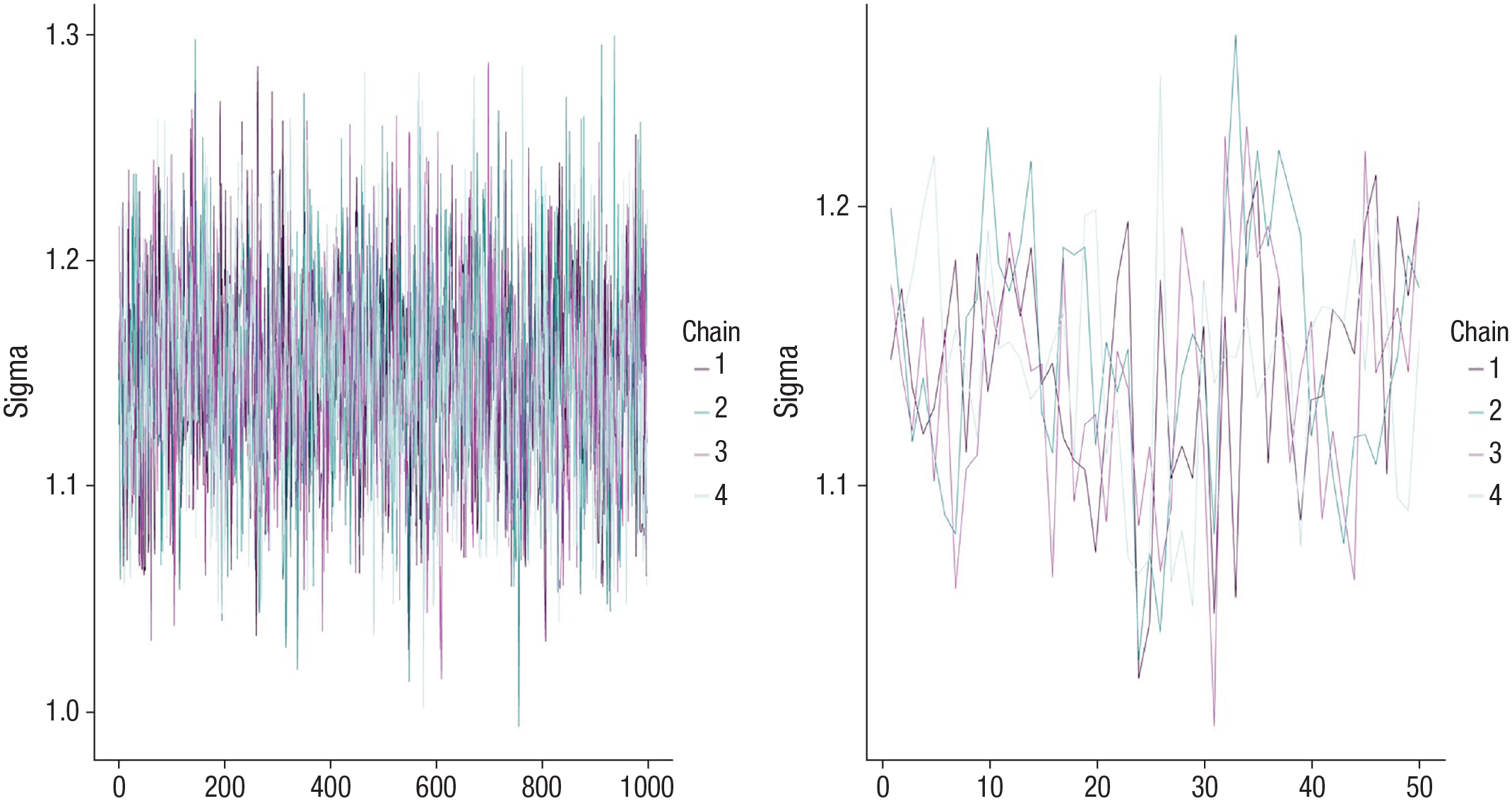
Trace plot indicating that the chains mixed (left) and a poorly mixed trace plot showing clear signs of separation across chains (right).

Assessing model fit

To assess whether our model fits the data well, we perform a posterior predictive check by simulating new values from the joint posterior distribution for our outcome and then compare these with the observed data. If our model fits the data well, the distribution of simulated outcome values should closely resemble the distribution of observed outcomes in our data set. Such a simulation can be easily carried out and plotted via the pp_check() command, which in our case, produces the plot in Figure 4.

Fig. 4.

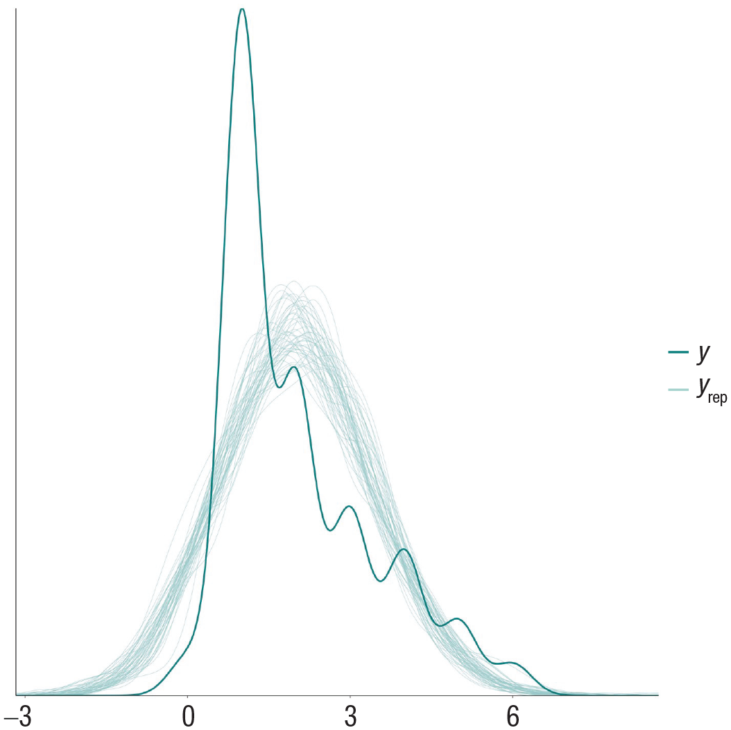
Posterior predictive check of the model predicting alcohol intoxication with a Gaussian distribution. The line corresponding to y represents the observed data, and the lines corresponding to y_rep represent the distributions generated by simulating from the model.

We can see that our model does not fit the data at all because the model-predicted data all follow a normal distribution, whereas the observed data follow a right-skewed distribution, and the central tendency of both distributions differs. This should be hardly surprising to us. First, statisticians have warned against the use of analyzing Likert-scale items with linear regression for decades and have recommended to use ordinal models instead (Coombs, 1960). Second, we need to consider the data-generating process of alcohol-intoxication reports. It is reasonable to assume that by and large, subjective alcohol intoxication increases as people consume additional alcoholic drinks. This suggests a sequential process wherein higher levels of alcohol intoxication are reached only after lower levels were reached earlier in the drinking episode. In responding to the ordinal alcohol-intoxication item, participants are attempting to quantify their level of alcohol intoxication (which may well be linear) by choosing among rank-ordered categories. Choosing between, for example, “very” and “very much” reflects a nonlinear threshold in which the probability of choosing the greater option increases slowly at first, then very quickly after some threshold, and then declines as the probability of choosing the next response option increases. Luckily, such a sequential ordinal model (Tutz, 1991) can be easily implemented in brms (Bürkner & Vuorre, 2019) by specifying family = sratio. Let us fit our updated model with a sequential ordinal outcome distribution and perform another posterior predictive check (Fig. 5):

Fig. 5.

Posterior predictive check of the model predicting alcohol intoxication with a sequential ordinal distribution. The line corresponding to y represents the observed data, and the lines corresponding to y_rep represent the distributions generated by simulating from the model.

We can see that this model fits our data much better, which is unsurprising given that it more accurately represents a plausible data-generating process. Because the Rhat values and effective sample sizes look good too, we proceed with interpreting the results of our model.

Bayesian inference

Remember that the posterior distribution is the product of our prespecified prior distribution and the likelihood (i.e., data). We can plot the posterior distribution with the mcmc_plot() command (Fig. 6).

Fig. 6.

Posterior distribution of the fixed main effect of self-control demands on alcohol intoxication. Plotted on top of the distribution is the 95% Bayesian credible interval.

Here, we learn that self-control demands on drinking days do not appear to be associated with alcohol intoxication (b = 0.05, 95% credible interval [CI] = [–0.11, 0.21]). Because this is an ordinal model, we need to exponentiate these values to learn by how many points alcohol intoxication increases as demands increase by 1 SD (OR = 1.05, 95% CI = [0.90, 1.23]). Whereas this would be the end of many frequentist analyses (“not significant”), the posterior distribution reveals more than might be immediately obvious. Recall that we specified a priori that we believe with 95% certainty that the effect size lies somewhere between an increase or decrease of 2 points. You can see that once we updated our beliefs by adding the data to the model, this uncertainty has decreased considerably, and we can now be 95% certain that the effect lies somewhere between a decrease of ≈0.1 points and an increase of ≈0.2 points. Thus, we can conclude that most likely, the effect is trivially small, but a miniscule plausibility of a small-but-meaningful effect in the expected direction remains.

If we wanted to calculate a Bayes’s factor for the hypothesis that the effect of self-control demands on alcohol intoxication is unequal to 0, we would compare a model including demands as a fixed effect (alc.intox ≈ 1 + demands + (1 + demands | PID)) with a null model without it (alc.intox ≈ 1 + (1 + demands | PID)). We can then feed both models into the bayes_factor() command to quantify the evidence for our hypothesis (Schad et al., 2022). We learn that the Bayes’s factor in favor of our hypothesis (BF₁₀) is 0.10, or 1 in 10, which means that the data provide 10 times more support for the null hypothesis than for our informative hypothesis. However, when using default brms priors, the Bayes’s factor in favor of H₀ is only 4.12, illustrating the importance of preregistering one’s priors.

Running Example 2: Fitting Models With Complex Outcome Distributions

For our second example, we explore whether people are more likely to drink and consume more drinks on days they reported higher self-control demands. Number of alcoholic drinks consumed is a count variable because it can take on only nonnegative integer values. Count variables are often modeled using the Poisson or negative binomial distribution. However, number of drinks consumed in EMA data tends to be zero-inflated because even regular drinkers tend to abstain on 50% to 80% of days (Dora et al., 2022), which implies a higher number of zeroes than expected by the Poisson or negative binomial distribution. Such data can be accounted for by using mixture models. For example, a zero-inflated model represents the outcome as a count distribution but with additional expected zeroes. A hurdle model first predicts the probability of not drinking and then separately predicts the number of drinks consumed on drinking days. Based on our experience predicting alcohol use in EMA data, a hurdle model with a negative binomial distribution for the nonzero values is often best matched with the data-generating process for daily alcohol use. ⁴ However, an important first step in analysis is to choose and compare various outcome distributions. In our own work predicting the number of drinks in EMA data, we often sequentially compare zero-inflated and hurdle Poisson or negative binomial models, choosing the simplest distribution that best fits the data. We first specify some weakly informative priors, which are based on earlier preregistered analyses of alcohol use predicted by affect (Dora et al., 2022). Because this model uses a logit link, we need to specify the log of our priors. For example, if we believe that participants on average consume ≈4.5 drinks ± 2.7 drinks per drinking episode with 95% probability (fixed intercept), we need to specify a normal(1.5, 0.3) prior. If we believe that the effect of demands on the number of drinks per drinking episode (fixed slope) should be somewhere between ±3 drinks, we need to specify a normal(0, 0.5) prior:

Next, we fit our brms model. We use the bf() command to easily specify two separate parts of our model, one predicting the zero values (i.e., whether or not drinking occurs; “hu”) and one predicting the nonzero values (i.e., how many drinks are consumed on drinking days; “alc.drinks”):

We check the trace plots to make sure that the chains mixed, ensure that Rhat values are close to 1 and effective sample sizes are adequate, and perform a visual posterior predictive check (Fig. 7), which shows that the model fits the data well.

Fig. 7.

Posterior predictive check of the hurdle model predicting number of alcoholic drinks with a negative binomial distribution for the nonzero counts. The line corresponding to y represents the observed data, and the lines corresponding to y_rep represent the distributions generated by simulating from the model.

We learn that demands are not associated with the odds of drinking on any given day (OR = 0.85, 95% CI = [0.47, 1.48]), nor are they associated with the number of drinks on drinking days (rate ratio [RR] = 0.99, 95% CI = [0.91, 1.07]). Nonetheless, we can see that the uncertainty around the effect on the count (i.e., nonzero) portion of the model is much smaller than the effect on the logit (i.e., zero) portion. Thus, we learn that we can be much more confident that higher self-control demands are not associated with drinking quantity (conclusive) than that they are not associated with the likelihood to drink (inconclusive) because meaningful effect sizes in both directions retain posterior probability. We can visualize this conclusion by plotting prior and posterior distributions on top of one another (Fig. 8), which shows the improvement in posterior precision of the count portion of the model, relative to the very minor improvement in the hurdle portion.

Fig. 8.

Prior and posterior distributions for the effect of demands on the daily likelihood to drink (left) and the number of drinks consumed on drinking days (right).

One question you might ask yourself at this point is to what extent the priors we chose influence the results. This always depends on the chosen priors and the amount of data you have available. As a rule of thumb, less informative priors will influence the results less, and all priors will influence the results less when more data are available. For example, in the hurdle model we fitted above, let us replace our weakly informative priors on the fixed effects with uninformative flat priors that distribute equal prior probability to effects ±3. This hardly affected the result for drinking quantity (RR = 0.99, 95% CI = [0.91, 1.07]), but the results for the likelihood to drink shifted somewhat (OR = 0.76, 95% CI = [0.36, 1.54]). Thus, in this example, the prior did not matter much for the substantive interpretation of the results, but you can imagine how this might change the conclusion in other applied settings. Here, the null result for drinking likelihood is still conclusive, and the uncertainty around the inconclusive result for drinking quantity is slightly bigger, meaning meaningful effect sizes larger and smaller than zero retain posterior probability.

As we argued above, we recommend using weakly informative priors and hence trust the results of that analysis more.

Although we are mostly interested in the fixed effects of our mixed-effects models, to better understand the results of our models, it is often useful to explore the random per-participant effects in our EMA data. For example, in case of null results, this helps us to understand whether there is potentially a subsample of participants who display the hypothesized effect. This could imply that an important between-persons moderator was missed that could explain for whom we should and should not expect the theoretical prediction to hold true. One way to do this is with the help of the tidybayes package (Kay, 2022). In this case, we have plotted the random per-participant effects of demands on the number of drinks consumed during drinking episodes for 10 of our participants (it is hard to plot slopes for hundreds of participants in a visually clear way; Fig. 9). We can see that the slopes differ somewhat, and especially, the intercepts differ substantially between participants. This type of plot can help us learn to understand what is going on in our data.

Fig. 9.

Per-participant random slopes (in black) surrounding the fixed effect (in gray) for the effect of perceived self-control demands on the number of drinks consumed during drinking episodes.

Running Example 3: Accounting for Missing Data in Our Bayesian Models

For our third example, we demonstrate how to account for missing data in Bayesian models using multiple imputation (MI). We would like to predict whether people are more likely to experience negative alcohol-related consequences following drinking on drinking days they reported higher self-control demands. Commonly, EMA researchers assess multiple alcohol consequences and then sum them for each drinking episode so that a higher score reflects more reported consequences (Wray et al., 2014). Because these “variety scores” ignore the uniqueness of each consequence (e.g., experiencing a hangover vs. injury) and reflect an assumption that all consequences are interchangeable in severity (because each experience equally increases the sum score by 1), we prefer to predict each consequence by itself. Here, we show the analysis predicting the likelihood of experiencing a hangover. Because we expect the likelihood of experiencing a hangover to be higher after more intense drinking, we will additionally predict consequences from the number of drinks consumed.

Accounting for missing data

One common struggle for EMA researchers we have not yet addressed is missing data. EMA studies almost always contain some amount of missing data, either by design or to minimize participant burden (Rhemtulla & Little, 2012) or because of participant nonresponse (a meta-analysis found an average response rate of 72% to 77% across 126 EMA studies; Jones et al., 2019). MI, which describes the general approach to create multiple data sets in which we replace missing values with plausible values randomly drawn from distributions and then pool the results across these multiple data sets, is widely regarded as a state-of-the-art solution to address missing data (van Buuren & Groothuis-Oudshoorn, 2011). Although alternatives are available (e.g., full information maximum likelihood (FIML), in which we do not impute missing values but estimate the single most plausible value based on the observed data), MI has several advantages pertinent to the study of EMA data. First, MI has demonstrated greater efficiency in parameter estimation compared with maximum-likelihood-based approaches (Enders, 2017). Second, modern MI methods have been designed to accommodate complex multilevel and nonlinear design (i.e., interactions and polynomial effects; Enders et al., 2020), both of which are central to the structure of EMA data and hypotheses of EMA design. Third, FIML accounts for data missing only on Y but not X at the lowest level of clustering, meaning it uses listwise deletion for any observation that is missing a value on a predictor.

Although a full review of imputing missing data that is nested in clusters (e.g., nested in participants in the case of EMA) is beyond the scope of this tutorial, here we show how we can easily fit a model on multiple imputed data sets with brms and how pooling inferences across these submodels is straightforward in the Bayesian framework. For example, here we could perform a quick-and-dirty ⁵ MI with the mice package (van Buuren & Groothuis-Oudshoorn, 2011) using the following code:

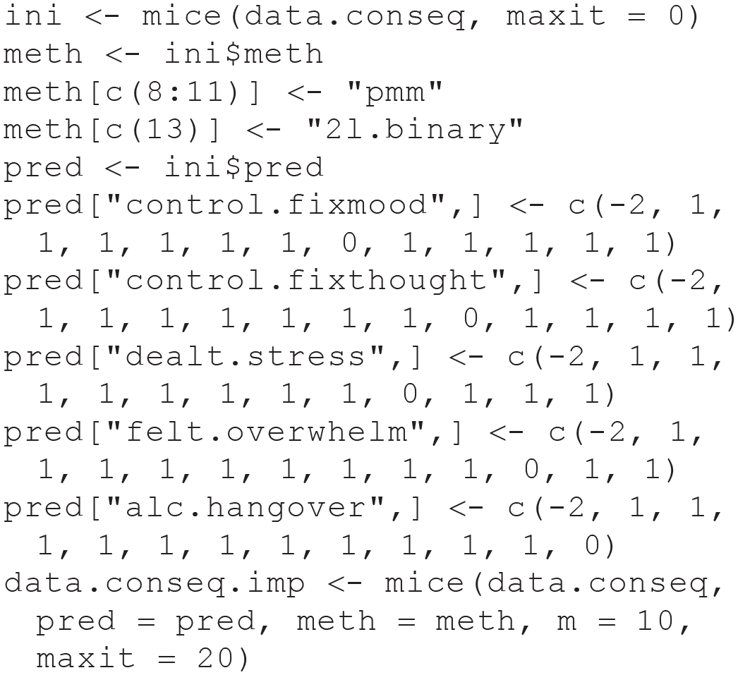
We use the data.conseq.imp object, which contains the 10 imputed data sets, in our model fitting below. Consequences were either endorsed or not endorsed for each drinking episode, meaning they are a binary outcome that we model with the bernoulli() family. Once more, we need to remember that our priors are on the log scale. Our priors specify that we believe that a hangover is experienced roughly every five drinking episodes at average levels of demands and drinks and that experiencing a hangover would be no more or less likely than 3 times for any increase in 1 SD in demands or one alcoholic drink:

We can use the brm_multiple() command to simply fit our model on multiple data sets:

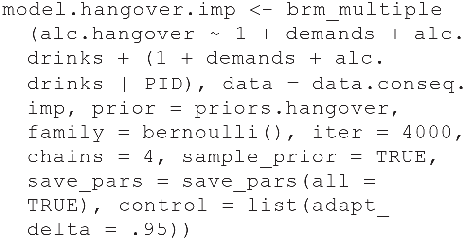
After fitting this model, brms warns us that parts of the model may not have converged as indicated by Rhat values larger than 1.05. Fitting a model on multiple data sets often results in false-positive convergence warnings because the chains for each data set may not overlap even when the model converged in each individual data set. We can confirm that the model converged by inspecting the individual Rhat values via model.hangover.imp$rhats, which clarifies that the Rhat values in each of the data sets are exactly 1. We can also perform a posterior predictive check on our brm_multiple() object; however, this will perform the check in only one of the imputed data sets (Fig. 10). Whereas pooling results across multiple frequentist models is not straightforward and can lead to biased inferences (Zhou & Reiter, 2010), in a Bayesian analysis, we can achieve a pooled inference by simply combining the posterior draws of the submodels. Once again, this results in a single posterior distribution (Fig. 11).

Fig. 10.

Posterior predictive check of the model predicting the likelihood of reporting a hangover. The line corresponding to y represents the observed data, and the line corresponding to y_rep represents the distribution generated by simulating from the model.

Fig. 11.

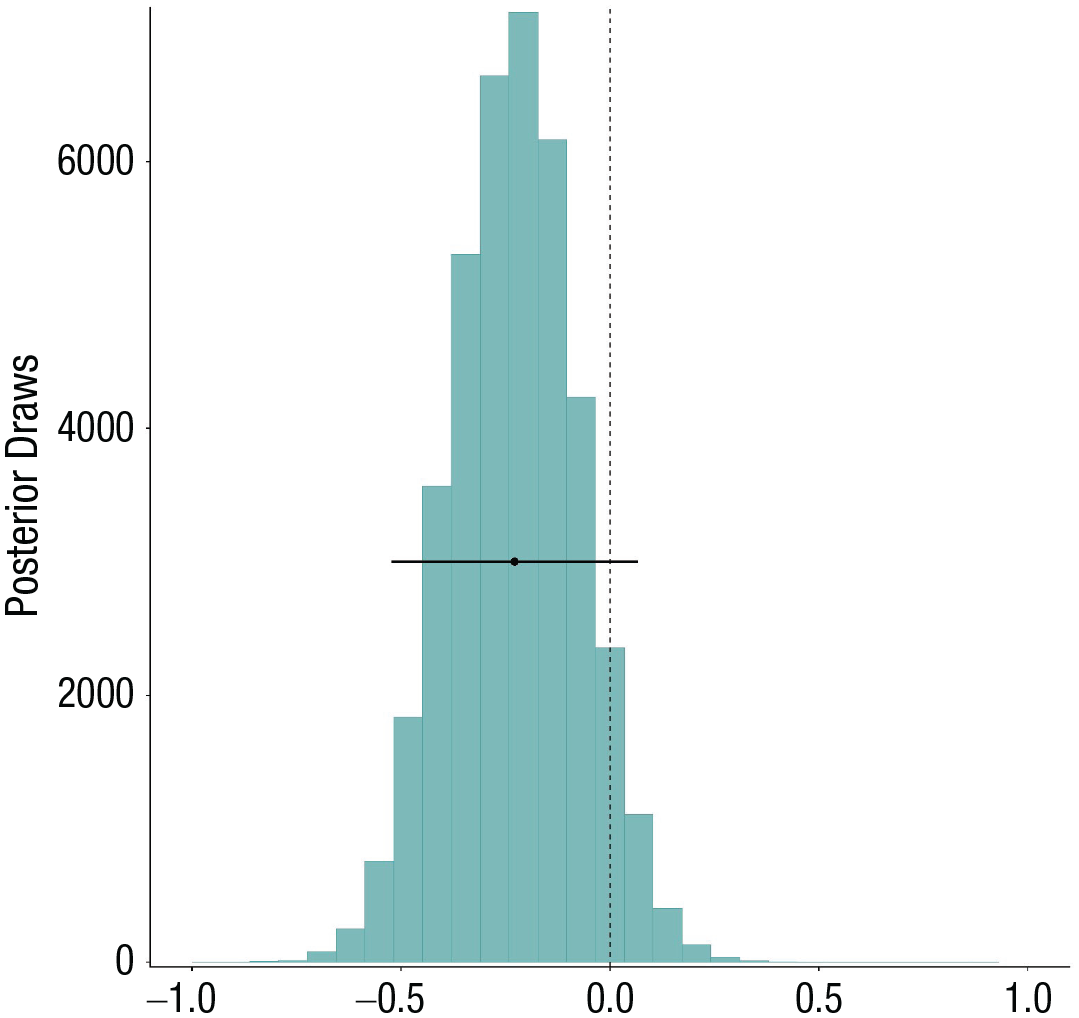
Posterior distributions of the fixed main effect of self-control demands on the likelihood to report a hangover. Plotted on top of the distribution is the 95% Bayesian credible interval.

We can see that according to a frequentist interpretation of the results, demands are not significantly associated with the likelihood of experiencing a hangover (OR = 0.79, 95% CI = [0.59, 1.07]). However, note that the CI is very wide here, indicating high uncertainty regarding the population-level effect size. In a Bayesian analysis, there is nothing magical about the value of 0 (or 1 in the case of OR). Whether this result provides evidence in favor of or against demands being associated with a reduced likelihood to experience a hangover the same day depends on what effect sizes we consider meaningful. For example, with the following code, we can realize that the posterior probability that a 1 SD increase in demands is associated with at least a 10% lowered likelihood to experience a hangover (assuming this is the smallest effect size we care about) is 80%:

The posterior probability that it is associated with at least a 20% lowered likelihood is only 56%. On the other hand, the posterior probability that the effect is positive is only 7%. Thus, controlling for the number of drinks participants consumed, the data overall provide some evidence that participants are slightly less likely to report a hangover on days they report higher self-control demands. The uncertainty in this conclusion is large, and thus, more data are required in the future to improve our confidence in this conclusion.

Unsurprisingly, number of drinks consumed was a consistent predictor of consequences. For example, our model estimates that with every additional drink, the likelihood of reporting a hangover increased by 21% (95% CI = [11%, 32%]. Because this may be hard to interpret, we like to plot this effect with the conditional_effects() command (Fig. 12). The plot shows that our model estimates that hangovers are rare even after five drinks and that it takes roughly 15 drinks to reach 50% probability. But we can also see that the uncertainty interval widens with increasing numbers of drinks because those are less often reported. Thus, our main conclusion from this result is that contrary to previous findings indicating that hangover severity declines with age (Tolstrup et al., 2014; Verster et al., 2021), college students in our data sets seem to be much more immune to hangovers than the authors of this article.

Fig. 12.

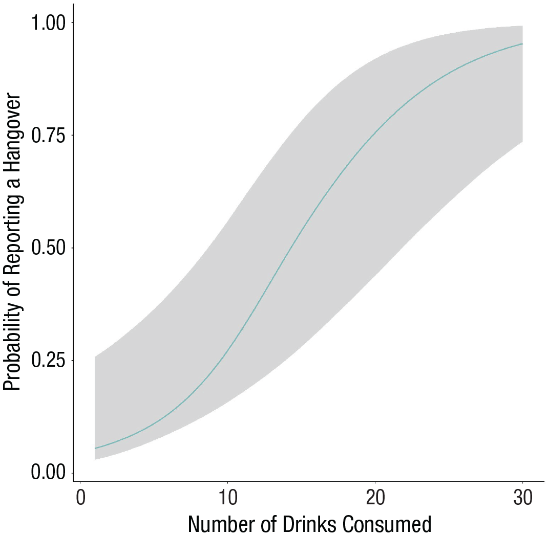
Effects plot displaying the estimated increased probability to report a hangover with additional alcoholic drinks consumed.

In summary, the results of our Bayesian analysis are more consistent with a recent EMA study (Walters et al., 2018) and do not corroborate two earlier studies that reported such associations (DeHart et al., 2014; Muraven et al., 2005). The current study does not provide support for an association between perceived self-control demands and alcohol use among college students. In the case of subjective alcohol intoxication, a Bayes’s factor provided 10-fold evidence against such a prediction.

Discussion

In the present tutorial, we aimed to provide a gentle introduction to how EMA data can be analyzed using Bayesian (generalized) mixed-effects models. We presented several strengths of the Bayesian approach for EMA data analysis. These are (a) how weakly informative priors aid convergence for models with random effects, (b) how weakly informative priors reduce the risk of overestimating the true effect size, and (c) how imputation of missing data can be implemented in a Bayesian framework. However, we argue that the Bayesian approach has additional advantages that are especially suitable and important when analyzing EMA data, which are expensive and time-consuming to collect. Specifically, Bayesian models de-emphasize mindless conclusions based on defaults and instead emphasize prespecifying a prior belief for each model parameter and deciding which effect sizes researchers deem plausible and meaningful before conducting their analysis. This is especially compatible with an Open Science perspective (Munafo et al., 2017), in which it is important to be transparent about what one expected from one’s data analysis before conducting a study. Moreover, by quantifying and presenting the uncertainty of models after analysis, the Bayesian perspective encourages researchers to provide interpretations of their models that are more closely grounded in their data rather than treating significance as a license to interpret their effects however they wish (Cohen, 1994; Cortina & Landis, 2011). This also provides a better understanding of when results provide strong evidence in favor of the presence or absence of an effect and as when results turn out to be inconclusive.

There are many theoretical and methodological issues in EMA research that we have not addressed. First, it is critical to harmonize one’s statistical test with one’s theoretical prediction (Kaurin et al., 2023), especially when it comes to the timescale at which hypothesized associations play out. Bayesian EMA models allow tremendous flexibility in modeling multiple timescales from contemporary or lagged associations at multiple lags to modeling trajectories within and across days. Alternatively, one may want to estimate an autoregressive correlation or an autoregressive moving average (Hamaker & Dolan, 2009) to model temporal dynamics in a variable. Location-scale models allow prediction of not only levels but also variation (Williams et al., 2019). You might want to apply growth-curve modeling (Armey et al., 2011) or survival analysis (ten Broeke et al., 2020) to your EMA data. All of these modeling procedures and more are implemented in brms along the vast array of outcome distributions, enabling you to perform all possible EMA analyses in the context of one software package, which makes learning brms an extremely efficient and rewarding endeavor. An advantage of fitting such complex models in a Bayesian framework is once more that priors help with parameter estimation and model convergence. One potential limitation of (generalized) linear mixed-effects models worth highlighting is that when studying lagged associations, these models do not account for the unequal time that passed between two consecutive EMA surveys. Recently, some work has been done to develop continuous-time models in which the lagged association decays over time (because it is reasonable to assume that any association that exists should get weaker as more time passes between two surveys). As of the time of writing this tutorial, it is hard to guess to what extent the discrete-time assumption biases inferences because simulation studies have come to different conclusions (De Haan-Rietdijk et al., 2017; Loossens et al., 2021). Continuous-time models such as the Ornstein-Uhlenbeck model, which has been used to analyze EMA data (Nowak et al., 2023), are currently not implemented in brms but can be specified in Stan, the infrastructure on which the package was built.

This tutorial provided a hands-on guide to Bayesian mixed-effects modeling of EMA data to EMA researchers new to Bayesian data analysis and highlights the immense flexibility the brms package gives researchers when analyzing a variety of outcomes. In reiteration, the steps we discussed are (a) defining our model; (b) defining outcome distributions and prior probability distributions for the parameters of interest, which involves consideration of the data-generating process and the expression of beliefs of the plausibility and meaningfulness of effect sizes; (c) fitting the model in brms; (d) assessing model convergence and model fit; and (e) drawing inferences via posterior distributions and Bayes’s factors. In this tutorial, we have not covered every aspect of Bayesian data analysis or the analysis of EMA data. To those readers who would like to dive deeper into Bayesian data analysis, we recommend to start with the textbook by McElreath (2020) and an annotated reading list by Etz and colleagues (2018).