Sage Journals: Discover world-class research

Abstract

Psychological science is moving toward further specification of effect sizes when formulating hypotheses, performing power analyses, and considering the relevance of findings. This development has sparked an appreciation for the wider context in which such effect sizes are found because the importance assigned to specific sizes may vary from situation to situation. We add to this development a crucial but in psychology hitherto underappreciated contingency: There are mathematical limits to the magnitudes that population effect sizes can take within the common multivariate context in which psychology is situated, and these limits can be far more restrictive than typically assumed. The implication is that some hypothesized or preregistered effect sizes may be impossible. At the same time, these restrictions offer a way of statistically triangulating the plausible range of unknown effect sizes. We explain the reason for the existence of these limits, illustrate how to identify them, and offer recommendations and tools for improving hypothesized effect sizes by exploiting the broader multivariate context in which they occur.

Keywords

hypothesis multivariate statistics effect size correlation sampling

Recent years have witnessed increased sophistication in the formulation and testing of hypotheses in psychology and its allied disciplines (Cumming, 2013). As part of improvements to research practices, psychologists pushed further the enrichment of hypotheses with approximate effect sizes. Doing so allows for a priori estimations of a required sample size (Cooper & Findley, 1982), helps to preemptively separate associations considered trivial in size from more substantial ones (Fritz et al., 2012), and in Bayesian analysis, helps to define one’s priors (Wagenmakers et al., 2018). Unsurprisingly, there is much debate about the question of what effect sizes are reasonable to expect. For example, it may be difficult to approximate an effect size associated with a novel hypothesis, and it may be challenging to state a priori whether the size of an effect in one context (e.g., in lab settings) will be the same elsewhere (e.g., in field settings; Giner-Sorolla et al., 2023; Greenwald et al., 2015). Simultaneously, methods of obtaining more accurate estimations of population-level effects, such as meta-analysis and meta-analytical structural equation modeling, have witnessed an increase in sophistication and popularity (Jak & Cheung, 2020; Johnson, 2021).

Much of the existing discussion about appropriateness of hypothesized effect sizes revolves around the theoretical basis for such claims or what empirical precedent exists. For example, a small effect size that affects humanity at large may be considered equally or more important than a large effect size that occurs among a specific subpopulation only. Furthermore, the typical magnitudes of effect sizes may vary across subdisciplines and paradigms, and size category labels may need to take such contingencies into account (Cohen, 1988; Funder & Ozer, 2019). We propose that there is another and more fundamental issue, underappreciated in quantitative psychology, that should be considered within this ongoing discourse: There are mathematical limits to the effect sizes that may exist in a population (and corresponding samples), and these may be surprisingly restrictive.

Understanding these limits helps appreciate the importance of considering the size of a hypothesized effect in light of what reality permits, which may require an appreciation of smaller effect sizes. Furthermore, these limits render some hypotheses entirely impossible. We demonstrate the mathematical basis for such limits, offer guidance for evaluating whether a hypothesis is impossible, and then illustrate how effect-size limits may be determined. Note that this article is written with the aim to be accessible to quantitative psychologists at large—inclusive of psychologists who possess but limited knowledge of statistics—and we accordingly forewarn the expert reader of our leisurely pace through the various arguments, equations, and examples. Practical recommendations and links to online tools are located in the latter half of this article.

Hypotheses as Statements About Correlation Matrices

A helpful way to think about hypotheses in quantitative psychology is to treat them as statements about presumed correlation matrices that describe a population in question. This is perhaps easiest to see for hypotheses that postulate simple associations between continuous variables, such as “Higher levels of social inclusion come with lower levels of anxiety,” for which one would accordingly expect a nonzero correlation—here a negative one in particular—between the two measured variables. A similar situation applies to hypotheses about group differences, such as “First-year students experience more anxiety than second-year students,” which essentially means that some level of covariance, and hence correlation, is expected to occur between anxiety and the dichotomous “student year” variable. Subsequent empirical studies, in turn, serve to test these predicted population-level correlations.

The above hypotheses are ordinal; that is to say, they postulate the sign of correlation but not its magnitude. There has been a disciplinary move away from such ordinal hypotheses toward more precise ones. For example, a researcher may hypothesize not merely that higher levels of social inclusion come with lower levels of anxiety but also that this association is “weak,” “moderate,” or “strong,” for example, corresponding to absolute correlations of around $r = . 1$ , $r = . 3$ , and $r = . 5$ (Cohen, 1988), respectively. Likewise, rather than merely hypothesizing that first-year students experience more anxiety than second-year students, a researcher may propose that the corresponding difference is “small,” “medium,” or “large,” corresponding to mean differences of 0.2 SD, 0.5 SD, and 0.8 SD (i.e., Cohen’s d; Cohen, 2013; Sawilowsky, 2009). These effect sizes may be explicitly mentioned as part of the hypotheses, or they may be postulated in the power analyses of corresponding studies.

To represent the above effect sizes into a correlation matrix, it is helpful to first define various concepts. For starters, the (population) “covariance” between Variables A and B is defined as

c o v (A, B) = \frac{1}{N} \sum_{i = 1}^{N} (A_{i} - \bar{A}) (B_{i} - \bar{B}) .

(1)

The covariance of a variable “with itself” (e.g., exchanging $B_{i} - \bar{B}$ for $A_{i} - \bar{A}$ ) is that variable’s variance, denoted as $v a r (A)$ or $v a r (B)$ . These covariances can then be transformed into correlations, r, by expressing covariance between two variables as a “proportion” of their variances:

r_{A B} = \frac{c o v (A, B)}{\sqrt{v a r (A) \cdot v a r (B)}} .

(2)

A corresponding correlation—or normalized covariance—matrix M for two or more variables, labeled $X_{1}$ through $X_{k}$ , where k is the number of variables, is then given by

M = r_{i j} \in ℝ^{k \times k}

(3)

diag (M) = 1

(4)

M = M^{T}

(5)

| r_{i j} | \leq 1 \forall (i, j) .

(6)

Specifically, this correlation matrix M is square with k rows and k columns. The diagonal contains the correlations of a variable with itself, which equals 1; its off-diagonal entries contain real numbers that represent the strength and direction of correlation. The correlation matrix is diagonally symmetric because any covariance between $X_{i}$ and $X_{j}$ is the same as the covariance between $X_{j}$ and $X_{i}$ . These correlations must lie between −1 and 1, representing perfect negative and positive correspondence, respectively.

One of the benefits of using the correlation matrix is that the effect size can be directly incorporated in it. For example, Table 1 represents the hypothesis that level of social inclusion has a moderately strong negative association with level of anxiety (i.e., $r = - . 30$ ).

Table 1.

A Simple Hypothesis

	Inclusion	Anxiety
Inclusion	1	−.30
Anxiety	−.30	1

The same can be done for the example hypothesis that postulated between-groups differences in anxiety for first- and second-year students after transforming Cohen’s d to Pearson r (assuming equal group sizes, normality, and variance homogeneity; Cohen, 2013):

r = \frac{d}{\sqrt{d^{2} + 4}} .

(7)

This can be extended to situations that involve more than two variables, such as in the two near-identical hypotheses, Hypotheses 1 and 2, in Table 2. For example, a researcher of nostalgia—a sentimental longing or wistful affection for the past (Sedikides et al., 2008) that is characterized by mixed or “bittersweet” feelings—may hypothesize that trait nostalgia (variable $X_{1}$ ) is associated with higher positive (variable $X_{2}$ ) and negative (variable $X_{3}$ ) affect, whereas positive and negative affect are themselves inversely correlated. This hypothesis seems reasonable: Recent work emphasizes that nostalgia mixes positive and negative affect (Wildschut & Sedikides, 2020). Furthermore, a recent meta-analysis showed that negative and positive affect are inversely related to each other, with a disattenuated coefficient of $r = - . 59$ (Busseri, 2018).

Table 2.

Example Hypotheses 1 and 2

Hypothesis 1		$X_{1}$	$X_{2}$	$X_{3}$
		(Nostalgia)	(PA)	(NA)
$X_{1}$	(Nostalgia)	1	.50	.50
$X_{2}$	(PA)	.50	1	−.59
$X_{3}$	(NA)	.50	−.59	1
Hypothesis 2		$X_{1}$	$X_{2}$	$X_{3}$
		(Nostalgia)	(PA)	(NA)
$X_{1}$	(Nostalgia)	1	.44	.44
$X_{2}$	(PA)	.44	1	−.59
$X_{3}$	(NA)	.44	−.59	1

Note: PA = positive affect; NA = negative affect.

The only difference between the two versions of this hypothesis is that Hypothesis 1 proposes slightly larger correlations for nostalgia with positive and negative affect ( $r = . 50$ ) than Hypothesis 2 ( $r = . 44$ ). Yet it turns out that only Hypothesis 2 is viable; there cannot be a population (or sample for that matter) that could support Hypothesis 1. Hypothesis 1 is an impossible hypothesis. Furthermore, although Hypothesis 2 is possible when considering its three variables in isolation, it nonetheless turns out to be impossible if one considers the role of other variables in the population.

Why is Hypothesis 1 outright impossible? And why does Hypothesis 2 turn out to be impossible as soon as it is considered in a broader variable context? The correlations that nostalgia has are probably unrealistically strong. What determines such limits? And more generally, how might this temper the anticipation of effect sizes? We address these questions next.

Impossible Hypotheses

The issue regarding Hypothesis 1 can be formulated in a more general form: The presence of a correlation between two variables sets limits to how these variables might relate to another one. The explanation for this, and corresponding guidance on how to evaluate the impossibility or implausibility of hypotheses, requires a few steps. We start off by illustrating the issue for the case of the 3 × 3 correlation matrices mentioned above before moving to the general case for correlation matrices of any dimension.

Specific case: Our impossible hypothesis has an impossible geometry

An intuitively helpful feature of correlation coefficients is that one can think of them as representing the cosines of the angle between two variables’ axes (Gniazdowski, 2013). For example, two variables with a correlation of $r = . 00$ can be thought of as a set of perpendicular axes $(\cos 90^{\circ} = 0.00)$ , whereas a correlation of $r = \pm 1.00$ implies a coaxial arrangement $(\cos 0^{\circ} = + 1.00, \cos 180^{\circ} = - 1.00)$ . The $r = - . 50$ correlations from Hypothesis 1 correspond to an angle between the axis of variables $X_{1}$ and $X_{2}$ of $120^{\circ}$ ( $\cos 120^{\circ} = - 0.50$ ). Thus, the larger a correlation coefficient gets, the smaller the angle becomes between the corresponding variable axis, which follows from the fact that the inverse cosine is a strictly decreasing function.

Before we apply this reasoning to Hypotheses 1 and 2, first consider a case of three uncorrelated variables (i.e., $r = . 00$ ). The angles between each pair of these variables is $90^{\circ}$ , which can easily be represented in a three-dimensional space with three perpendicular axes, as shown in Figure 1a. To make things more interesting, we change the correlation that $X_{3}$ has with the other two into $r \sim \sim . 35$ , corresponding to an angle of $70^{\circ}$ with both the $X_{1}$ axis and the $X_{2}$ axis. (Note that we leave the null correlation between $X_{1}$ and $X_{2}$ unaltered.) This is still easily represented geometrically. All we have to do is rotate the $X_{3}$ axis toward the plane captured by the axis for $X_{1}$ and $X_{2}$ . If we do so sufficiently, then we can reduce the original $90^{\circ}$ angles to ones of $70^{\circ}$ (see Fig. 1b). We can go further on this path: We can increase the correlation that $X_{3}$ has with the other two variables to, say, $r = . 50$ , corresponding to $60^{\circ}$ angles, or all the way up to $r \sim \sim . 71,$ where the axis of $X_{3}$ lies in the plane spanned by $X_{1}$ and $X_{2}$ , at an angle of $45^{\circ}$ to each axis (see Fig. 1c). Enthusiastic as we are about our little game, let us try for correlation coefficients between $X_{3}$ with $X_{1}$ and $X_{2}$ of $r = . 80$ , corresponding to angles of just $37^{\circ}$ between $X_{3}$ and $X_{1}$ and between $X_{3}$ and $X_{2}$ . Alas, this is where our fun ends; there is no possible way to rotate the $X_{3}$ axis any closer to the $X_{1}$ axis and the $X_{2}$ axis simultaneously. With an angle of $90^{\circ}$ between the $X_{1}$ and $X_{2}$ axis, the smallest equal angles that the $X_{3}$ axis can have with them is $45^{\circ}$ to each. Accordingly, the largest positive correlation that can exist between $X_{3}$ with both $X_{1}$ and $X_{2}$ , assuming that $X_{1}$ and $X_{2}$ are themselves uncorrelated, is $r = \cos 45^{\circ} = 1 / 2 \sqrt{2} \approx . 71$ .

Fig. 1.

Geometrical illustration of a positive correlation limit.

However, this is only half of the story. In addition to positive correlation limits, there are also limits to negative ones, which can be found by trying to rotate the $X_{3}$ axis such that it creates the largest possible angles with the other two. In this case, we can achieve that by rotating the $X_{3}$ axis in the opposite direction—away from the $X_{1} X_{2}$ plane (see Fig. 2a). The largest angle that the $X_{3}$ axis can make with the other two ones occurs when it is turned, again, into the $X_{1} X_{2}$ plane, but this time in the opposite direction. This creates two angles of $135^{\circ}$ , corresponding to a most negative correlation coefficient of $r \approx - . 71$ , as shown in Figure 2b. For a formal discussion of these limits, see the Supplemental Material available online. Note that for other cases, the most positive and negative correlations may differ in both sign and magnitude.

Fig. 2.

Geometrical illustration of a negative correlation limit and the case of Hypothesis 2.

We first apply the same reasoning to Hypothesis 2. The correlation between positive affect and negative affect $r = - . 59$ corresponds to an angle of $126^{\circ}$ . The angle between the nostalgia axis and the positive-affect axis is $64^{\circ}$ $(r = . 44)$ , and the same is true for the angle between the nostalgia axis and the negative-affect axis. The axis that characterizes nostalgia thus nearly falls on the positive-affect and negative-affect plane (see Fig. 2c). In fact, rotated a little further, it would neatly split it at $63^{\circ}$ angles with the positive-affect and negative-affect axes. This would correspond to maximum correlations of $r = . 45$ , just above the correlations postulated under Hypothesis 2—which so far appears possible—but below that of Hypothesis 1—which is thus outright impossible.

Specific case: Our impossible hypothesis violates limits to multiple correlation

Aside from interpreting correlations geometrically, readers with a psychology background are probably familiar with interpreting these correlations as the square roots of the proportion of variance that two variables have in common. Indeed, the limits of $- 1$ and $+ 1$ that correlations have correspond to a maximum proportion of shared variance equal to 1 (or $100 %$ ). At first glance, it may seem that neither Hypothesis 1 nor Hypothesis 2 violates this limit; after all, each individual correlation coefficient lies between $- 1$ and $+ 1$ .

Yet a closer inspection reveals that Hypothesis 1 does prove problematic in this regard. Although neither the correlation between $X_{2}$ and $X_{1}$ nor that between $X_{3}$ and $X_{1}$ represent more than $100 %$ of variance accounted for individually, they nonetheless do so jointly. For the case of three variables, proportion of variance accounted for in one variable by the other two jointly is represented by the square of the multiple correlation coefficient (Neter et al., 1996), specifically:

R_{1}^{2} = \frac{r_{12}^{2} + r_{13}^{2} - 2 r_{12} r_{13} r_{23}}{1 - r_{23}^{2}} .

(8)

When we calculate the squared multiple correlation for each of the three variables in Hypothesis 1, we find that this value is 122% for nostalgia and 119% for both positive affect and negative affect. This is clearly impossible. For Hypothesis 2, on the other hand, we find values of 94%, 96%, and 96%, respectively—very high indeed but technically not impossible.

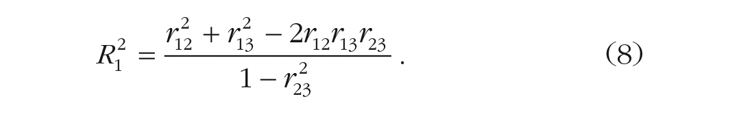
We can helpfully use Equation 8 to figure out what the minimum and maximum values are that a correlation coefficient can have by requiring $R_{i}^{2}$ and then solving for the coefficient of interest; Equation 9a illustrates this for the limits of a three-variable system:

r_{12} \leq r_{13} r_{23} \pm \sqrt{(r_{13}^{2} - 1) (r_{23}^{2} - 1)}

(9a)

r_{13} \leq r_{12} r_{23} \pm \sqrt{(r_{12}^{2} - 1) (r_{23}^{2} - 1)}

(9b)

r_{23} \leq r_{12} r_{13} \pm \sqrt{(r_{12}^{2} - 1) (r_{13}^{2} - 1)} .

(9c)

For example, assuming $r_{13} = . 50$ and $r_{23} = - . 59$ , as per Hypothesis 1, we find $- . 99 \leq r_{12} \leq . 40$ ; the value that $r_{12}$ can take must lie within these bounds. Indeed, Hypothesis 1 exceeds these limits. Applying the same to $r_{12}$ in Hypothesis 2, thus assuming $r_{13} = . 44$ and $r_{23} = - . 59$ , returns $- . 98 \leq r_{12} \leq . 47$ , which just includes the predicted value of $r_{12} = . 44$ . Thus, Hypothesis 2 appears to be possible.

One way to visualize the mathematical bounds dictated by Equation 8 is to realize that this equation defines the elliptical boundary of the pairs of $r_{12}$ and $r_{13}$ that satisfy $R^{2} \leq 1$ for any given $r_{23}$ (see the Suppelemental Material). Figure 3 illustrates what upper and lower values bound a correlation between two variables within any three-variable context.

Fig. 3.

Ellipses that enclose allowed values of $r_{12}$ and $r_{13}$ , shown for three values of $r_{23}$ : .0 (black), .7 (blue), –.9 (red). The dotted lines indicate $45^{\circ}$ . In orange, we show the permissible values for $r_{13}$ when $r_{23} = - . 9$ and $r_{12} = . 6$ ; for these values $- . 89 \leq r_{13} \leq - . 19$ .

General case: impossible hypotheses considering three or more variables

Examining whether hypotheses are impossible using squared multiple correlation may not have the intuitive appeal of the geometric interpretation explained earlier, but it has another desirable quality: It scales easily for any number of variables. In fact, Equation 8 that we used earlier to examine squared multiple correlations among three variables is a special case of (Neter et al., 1996)

R^{2} = {\vec{c}}^{T} M^{- 1} \vec{c} .

(10)

In Equation 10, $\vec{c}$ represents a column vector containing correlations that a variable of interest has with the others, and M represents the correlation matrix of these other variables with each other. We can apply Equation 10 to Hypotheses 1 and 2 and calculate multiple $R_{i}^{2}$ for each of their three variables.

The same can be done for correlation matrices with a larger number of variables. Consider the following example, loosely set to a social-identity context (Tajfel, 2010): A researcher studies social identification among English football fans with their various teams. Each participant will be asked to indicate their identification with three English teams: Manchester United, Liverpool, and Arsenal. The first two of these teams are allegedly fierce rivals, and one might accordingly expect a substantial negative correlation between identification with either team, say $r = - . 50$ . Less rivalry possibly exists between Arsenal and the other two teams, and one might accordingly expect social identification with Arsenal to correlate at a modest $r = - . 20$ with social identification for each of the other two teams. Our imaginary researcher knows of the power that common in-groups can have in bringing people together (Gaertner et al., 1993). In this case, the common in-group might be the English national team. Specifically, with the national team likely featuring some players from Manchester United, Liverpool, and Arsenal, our researcher anticipates that participants socially identifying strongly with their local team will also identify more with the national team, implying a positive correlation. We display this set of predictions in Table 3, in which Hypothesis 3 proposes a slightly higher set of correlations for identification with the national team (each $r = . 40$ ) than Hypothesis 4 (each $r = . 20$ ).

Table 3.

Example Hypotheses 3 and 4

Hypothesis 3		$X_{1}$	$X_{2}$	$X_{3}$	$X_{4}$
		(Manchester United)	(Liverpool)	(Arsenal)	(England)
$X_{1}$	(Manchester United)	1	−.50	−.20	.40
$X_{2}$	(Liverpool)	−.50	1	−.20	.40
$X_{3}$	(Arsenal)	−.20	−.20	1	.40
$X_{4}$	(England)	.40	.40	.40	1
Hypothesis 4		$X_{1}$	$X_{2}$	$X_{3}$	$X_{4}$
		(Manchester United)	(Liverpool)	(Arsenal)	(England)
$X_{1}$	(Manchester United)	1	−.50	−.20	.20
$X_{2}$	(Liverpool)	−.50	1	−.20	.20
$X_{3}$	(Arsenal)	−.20	−.20	1	.20
$X_{4}$	(England)	.20	.20	.20	1

Hypothesis 3 is impossible, and Hypothesis 4 appears to be possible. When we apply Equation 12 to these matrices, we find that the squared multiple correlations for Hypothesis 3 are impossibly large ( $R_{1}^{2} = 128 %$ , $R_{2}^{2} = 128 %$ , $R_{3}^{2} = 160 %$ , $R_{4}^{2} = 126 %$ ). For Hypothesis 4, they are fairly high but not impossible ( $R_{1}^{2} = 50 %$ , $R_{2}^{2} = 50 %$ , $R_{3}^{2} = 31 %$ , $R_{4}^{2} = 31 %$ ). If our researcher proposes that identification with local teams coincides with higher identification with the national team, then, within such a rivalrous context, the researcher can expect the corresponding effect sizes to be rather small.

Impossible Hypotheses in Light of Their Multivariate Populations

As the above section progressed, we discussed hypotheses with increasingly more variables. Many hypotheses in psychology feature only two or three key variables. Does that mean that only two or three need to be considered when evaluating the impossibility of a hypothesis? Unfortunately not. Note that hypotheses are statements about the relationship between one or more variables in a population and that this population is likely to be characterized by many more variables than just the ones that feature in the hypothesis. Although researchers may collect a sample that features only the key variables from their hypothesis, the variables’ relationships in this sample will represent those in the (multivariate) population from which the sample is drawn (albeit imperfectly, e.g., because of measurement error). The notion that hypotheses, although tested with samples, refer to populations has an important implication: Whether a hypothesized effect size turns out to be impossible will depend on both how it is related to the other key hypothesis variable(s) and how these key variables relate to others in the same population.

Earlier, in passing, we mentioned that although Hypothesis 2 seemed possible, it most likely is not. Likewise, Hypothesis 4, although seemingly possible, can probably not describe a real situation. Why is that the case? As alluded to above, the issue for both Hypotheses 2 and 4 is that their viability hinges on the magnitude of correlations with other variables in the population—whether measured or not. With each of the hypothesis variables featuring substantial maximum squared multiple correlations, the existence of correlations with other variables in the same population could quickly reveal them as impossible.

To illustrate, reconsider Hypothesis 2. A closer look at the literature suggests that among other things, dispositional nostalgia tends to have a positive correlation with another form of affect: loneliness. Specifically, research suggests that people turn to nostalgic reverie to soothe psychological and physical discomfort (Van Tilburg et al., 2018; Wildschut & Sedikides, 2020; Zhou et al., 2012), and the correlation between nostalgia and loneliness has been estimated at $r = . 14$ (Abeyta et al., 2020; Zhou et al., 2008). On the basis of prior work, we can also see that loneliness can be expected to correlate to positive affect and negative affect at $r = - . 56$ and $r = . 47$ , respectively (Neto, 2014). We add this new knowledge to our existing Hypothesis 2, which now contains three focal variables of interest (nostalgia, positive affect, negative affect) and one that that we merely add for context (loneliness; Table 4). We label our expanded version “Hypothesis 2*.”

Table 4.

Extended Example Hypothesis 2*

Hypothesis 2*		$X_{1}$	$X_{2}$	$X_{3}$	$X_{4}$
		(Nostalgia)	(PA)	(NA)	(Loneliness)
$X_{1}$	(Nostalgia)	1	.44	.44	.14
$X_{2}$	(PA)	.44	1	−.59	−.56
$X_{3}$	(NA)	.44	−.59	1	.47
$X_{4}$	(Loneliness)	.14	−.56	.47	1

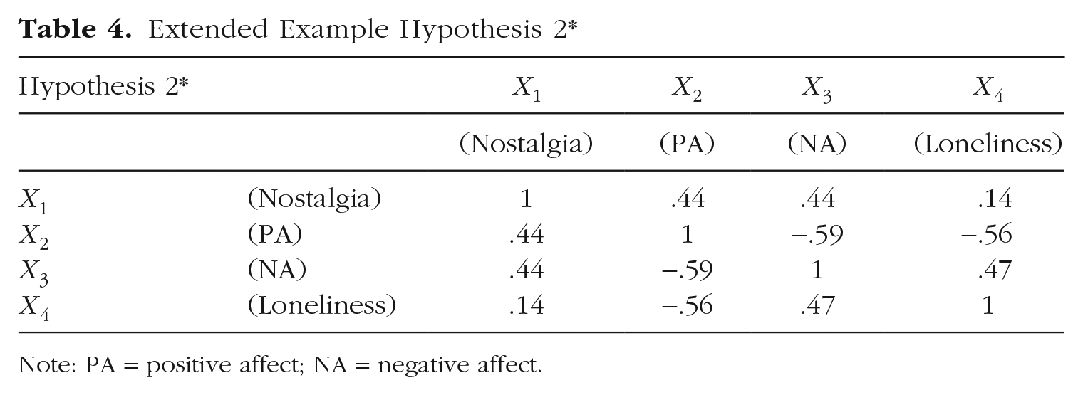
Note: PA = positive affect; NA = negative affect.

Calculating the squared multiple correlations for our variables now reveals that they exceed their limits ( $R_{1}^{2} = 103 %$ , $R_{2}^{2} = 102 %$ , $R_{3}^{2} = 103 %$ , $R_{4}^{2} = 135 %$ ). Knowing how nostalgia, positive affect, and negative affect are related to loneliness (provided we are confident about those correlations) tells us that we will never find our prediction that nostalgia correlates .44 to positive and negative affect confirmed.

The same reasoning applies to Hypothesis 4. Again, the squared multiple correlations quickly exceed their limits if another population variable is added regardless of whether we plan to sample it. Consider, for example, what happens if we consider an additional local football team: Tottenham Hotspur, an alleged fierce rival of Arsenal. We might reasonably expect individuals socially identifying with Arsenal to identify less with Tottenham Hotspur, much in the same way as was the case for Manchester United and Liverpool (Table 5). This renders our adjusted Hypothesis 4* impossible as a result ( $R_{1}^{2} = 128 %$ , $R_{2}^{2} = 128 %$ , $R_{3}^{2} = 128 %$ , $R_{4}^{2} = 128 %$ , $R_{5}^{2} = 160 %$ ). Thus, further integrating our prediction within a broader context in which these teams operate gives us a helpful but perhaps sobering vision of the actual feasibility of what we predicted. Clearly, one or more of the correlations in Hypotheses 4* and 2* must be unrealistic.

Table 5.

Extended Example Hypothesis 4*

Hypothesis 4*		$X_{1}$	$X_{2}$	$X_{3}$	$X_{4}$	$X_{5}$
		(Manchester United)	(Liverpool)	(Arsenal)	(Manchester United)	(England)
$X_{1}$	(Manchester United)	1	−.50	−.20	−.20	.20
$X_{2}$	(Liverpool)	−.50	1	−.20	−.20	.20
$X_{3}$	(Arsenal)	−.20	−.20	1	−.50	.20
$X_{4}$	(Manchester United)	−.20	−.20	−.50	1	.20
$X_{5}$	(England)	.20	.20	.20	.20	1

Using the above squared multiple correlation method to detect impossible correlations expresses the issue of impossible hypotheses in terms of the familiar concept of explained variances. Alternatively, researchers may have encountered situations in which they found that a correlation matrix failed to be positive definite, that the matrix thus produced negative eigenvalues, that the determinant of a matrix proved zero or negative, or that the matrix was singular (Marcus & Minc, 1988). These are symptoms of the same underlying problem: The correlation matrix in question is impossible (Lorenzo-Seva & Ferrando, 2021).

Identifying Effect-Size Limits

The above sections reveal that the limits to effect sizes within a multivariate context may be more restrictive than typically assumed. Psychology examines extensively, perhaps even entirely, variables from multivariate populations. An obvious question following from the above sections is what effect sizes, then, are more reasonable to expect. Existing empirical work can then help in figuring out whether a specific proposed effect is realistic or not by piecing together a population correlation matrix that contains the variables of main interest alongside other ones. Specifically, as shown above, knowing how a focal pair of variables relates to other variables in the population, for example based on existing research, may help to then approximate the strength of association between this focal pair even if there is no prior evidence of the association between the focal pair of variables themselves yet. How can one use this prior information to identify possible limits to effect sizes?

Size limits for a single hypothesized effect

The simplest form of hypothesis formulation is probably when a single effect size is proposed. For example, a researcher may seek to hypothesize a specific correlation for the tentative association between nostalgia and positive affect. As we have shown above, one can use knowledge about the wider multivariate context to get a better idea of what effect size is possible. For example, our hypothetical researcher might be aware that nostalgia and loneliness may correlate at around $r = . 14$ (Abeyta et al., 2020; Zhou et al., 2008), may expect that negative affect and nostalgia may correlate at around $r = . 40$ , and that loneliness and negative affect may correlate at around $r = . 47$ (Neto, 2014). Likewise, our researcher may have read that positive affect and negative affect can be expected to correlate at $r = - . 59$ (Busseri, 2018) and that positive affect and loneliness may correlate at $r = - . 56$ (Neto, 2014). Essentially, reading the existing literature gives our researcher some insight into how the key variables, nostalgia and positive affect, may relate to other variables in the population. The only thing the researcher does not know (conveniently so for our example) is how strong the correlation between nostalgia and positive affect might be (Table 6).

Table 6.

Estimating a Single Unknown Effect Size

		$X_{1}$	$X_{2}$	$X_{3}$	$X_{4}$
		(Nostalgia)	(PA)	(NA)	(Loneliness)
$X_{1}$	(Nostalgia)	1	$r_{12}$	.40	.14
$X_{2}$	(PA)	$r_{12}$	1	−.59	−.56
$X_{3}$	(NA)	.40	−.59	1	.47
$X_{4}$	(Loneliness)	.14	−.56	.47	1

Note: PA = positive affect; NA = negative affect.

Armed with knowledge about these other correlations, it is now possible for our researcher to narrow down the range in which the unknown effect size may fall. After all, its correlation value must not cause any of the squared multiple correlations to exceed 100%. Accordingly, we can solve Equation (10) for $R_{12}^{2}$ , where the a single correlation between nostalgia and positive affect is assumed unknown:

\begin{array}{l} (\begin{array}{l} r_{12} & 0.40 & 0.14 \end{array}) {(\begin{array}{l} 1 & - 0.59 & - 0.56 \\ - 0.59 & 1 & 0.47 \\ - 0.56 & 0.47 & 1 \end{array})}^{- 1} (\begin{array}{l} r_{12} \\ 0.40 \\ 0.14 \end{array}) \leq 1 . \\ \to - 0.897 \dots \leq r_{12} \leq 0.459 \dots \end{array}

Thus, if we can assume that the correlations obtained in prior studies give us an accurate impression of the population at large, then we know that the correlation between positive affect and nostalgia must lie between $r \approx - . 90$ and $r ~ ~ . 46$ . Effect sizes within this range will not cause the hypothesis to be impossible, to the extent that we have accurately and exhaustively considered other variables in the population. If our researcher suspects a positive association between nostalgia and positive affect, consistent with theorizing, then the researcher is thus wise to propose one in the range $. 0 \leq r \leq . 46$ .

Size limits for two hypothesized effects

It is far from uncommon for psychologists to formulate hypotheses about two associations rather just one. In our original nostalgia example, for instance, we predicted effect sizes for nostalgia’s association with both positive and negative affect. Can we estimate effect-size limits assuming that both are unknown? The answer is yes. Specifically, we need to solve

(\begin{array}{l} r_{12} & r_{13} & 0.14 \end{array}) {(\begin{array}{l} 1 & - 0.59 & - 0.56 \\ - 0.59 & 1 & 0.47 \\ - 0.56 & 0.47 & 1 \end{array})}^{- 1} (\begin{array}{l} r_{12} \\ r_{13} \\ 0.14 \end{array}) \leq 1 .

(12)

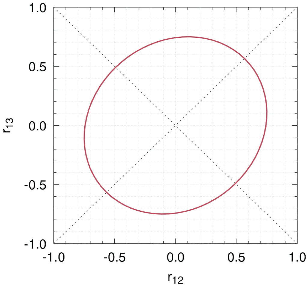
We can then plot the resultant inequality with two unknowns for ease of interpretation. Figure 4 displays the corresponding ellipse that encloses the possible values that these two correlations may take. This figure reveals that there exists a trade-off between the effect sizes one may hypothesize for $r_{12}$ and $r_{13}$ —as one effect size becomes more extreme, the limits to the second effect size become more narrow. The ellipse itself identifies pairs of effect sizes that result in squared multiple correlations of 1.0.

Fig. 4.

Ellipse that encloses possible values for $r_{12}$ and $r_{13}$ , given $r_{23} = . 14$ . See equation 12.

Of course, a similar approach can be adopted for cases in which three or more effect sizes need to be hypothesized. The downside is that clear visual guides such as Figure 4 are impossible to produce with a number of unknown variables greater than three.

Size limits for hypothesized group differences

The previous sections covered the existence of impossible hypotheses in the form of correlation matrices. These sections showed that effect-size limits may often be more restrictive than the typically assumed limits of $r = - 1.00$ and $r = 1.00$ for any individual correlation coefficient. We appreciate, however, that many researchers test hypotheses that seem different in form or context. Indeed, a large portion of psychological science is especially interested in comparing specific groups of individuals (e.g., participants who are randomly assigned to one of various experimental conditions), comparing clinical and nonclinical persons, and contrasting different demographic groups against each other. The magnitude of the tentative differences between such groups is typically expressed as the number of standard deviations that they differ from one another—Cohen’s d. As mentioned in our opening sections, Cohen’s d can be easily transformed into a correlation using Equation 7. The same tests of hypothesis impossibility and limits can then be employed to evaluate proposed effect sizes, as we did before for matrices that originally contained correlations already.

Consider, for example, a study in which a psychologist wishes to test if a gratitude intervention can help reduce state boredom. As part of this intervention, people list, on a daily basis, things they are grateful about for a period of several days (Emmonse & Mccullough, 2003; Sztachańska et al., 2019). This intervention is then compared against a condition in which participants listed memorable events instead. What is the possible range that the effect size can take? Published work on the impact of a gratitude intervention on boredom is absent at the time of this writing. However, both these variables have been independently examined in context of self-reported gratitude and well-being. Specifically, a meta-analysis showed that such gratitude interventions increase self-reported gratitude with a size of $d = 0.46$ and well-being by $d = 0.17$ (Davis et al., 2016). Furthermore, recent work suggests that state boredom and self-reported gratitude correlate at $r = - . 25$ (O’Dea et al., 2023) and that state boredom correlates at $r = - . 45$ with subjective well-being (operationalized as life satisfaction; Fahlman et al., 2013). Self-reported gratitude and well-being (again, operationalized as life satisfaction) can be expected to correlate at approximately $r = . 49$ (Kong et al., 2015).

After transforming the Cohen’s d values into correlation coefficients following Equation 7, we can complete most of the correlation matrix that approximates the effect sizes among the (e.g., dummy-coded) gratitude intervention, state boredom, self-reported gratitude, and well-being (Table 7).

Table 7.

Estimating a Single Unknown Effect Size for a Group Comparison

		$X_{1}$	$X_{2}$	$X_{3}$	$X_{4}$
		(Intervention)	(Boredom)	(Gratitude)	(Well-Being)
$X_{1}$	(Intervention)	1	$r_{12}$	.22 ( $d = 0.46$ )	.08 ( $d = 0.17$ )
$X_{2}$	(Boredom)	$r_{12}$	1	−.25	−.45
$X_{3}$	(Gratitude)	.22 ( $d = 0.46$ )	−.25	1	.47
$X_{4}$	(Well-being)	.08 ( $d = 0.17$ )	−.45	.47	1

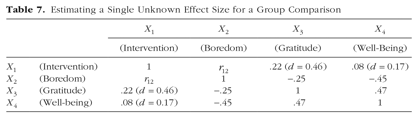
We can now use Equation 10 to compute the limits of $r_{12}$ by solving for $R^{2}$ ≤ 1, which gives $- . 92 \leq r_{12} \leq . 82$ . Transforming this back into Cohen’s d, we can expect that the effect of the gratitude intervention of boredom must lie between $- 4.57 \leq d \leq 2.88$ , assuming equal group sizes. Although this range is still rather large, it is more restrictive than the Cohen’s d values corresponding to the “uncorrected” $- 1 \leq r \leq 1$ range, which range from $- \infty$ to $+ \infty$ . Including correlations with additional population variables, if estimates are known, may further narrow down this range.

Practical Recommendations and Online Tools

Our article adds a tool to researchers’ statistical arsenal with two procedures. The first is a way to to tell researchers whether a hypothesis is possible on the basis of the squared multiple correlations of the included population variables. The second serves as advisory tool that tells researchers the range in which an effect size can be expected to fall after specifying an incomplete hypothesis—a population correlation matrix with at least one unknown. Both uses operate through Equation 10; Equation 8 serves the specific case of three variables. An interactive and easy-to-use web application featuring these tools is available at https://wapvantilburg.shinyapps.io/Hypothesis_Evaluation_Tool/.¹ There are various scenarios in which our evaluative and advisory procedures may aid researchers, discussed below. Note that we also highlight more specific extensions of our work in the Supplemental Material, including the link between the current work and “Voodoo” correlations (Fiedler, 2011; Vul et al., 2009), conventions on effect-size labels and categories, and experimental-design applications.

Use 1: testing whether a fully formed hypothesis is possible

The first use of our tool is a rather obvious one: Before finalizing power analysis, preregistering a study, and then conducting it, we recommend that researchers test whether their hypothesis is in fact possible. Doing so can prevent conducting a study that, from its onset, will inevitably cause the hypothesis to be empirically unsupported when it is statistically impossible. The abovementioned web application allows researchers to do this, as does Equation 10.

Use 2: examining how close hypothesized effect sizes are to their limits

This scenario may apply in at least two cases. First, researchers who have discovered that their hypothesis proved impossible may wish to scrutinize the specified correlations further. Any of the correlations specified in a hypothesis might in principle cause it to be impossible. Nonetheless, it may be helpful to see just by how much individual correlations require adjustment for the hypothesis to become possible. To examine this, a researcher could estimate ranges for each of the correlations in turn, each time treating it as unknown while retaining the others as originally specified. Doing so results in a matrix of possible correlation ranges against which the original correlations can then be compared. As an example, we performed this procedure on the impossible Hypothesis 1, which gave the ranges in Table 8.

Table 8.

Effect-Size Ranges for Hypotheses 1

		$X_{1}$	$X_{2}$	$X_{3}$
Hypothesis 1		(Nostalgia)	(PA)	(NA)
$X_{1}$	(Nostalgia)	1	.99 to .40	−.99 to .40
$X_{2}$	(PA)	−.99 to .40	1	−.50 to 1.00
$X_{3}$	(NA)	−.99 to .40	−.50 to 1.00	1

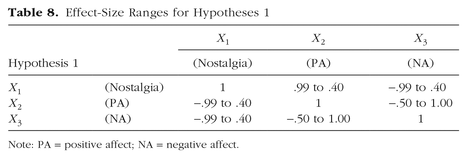
Note: PA = positive affect; NA = negative affect.

With this information at hand and, of course, mindful of existing theory and prior findings, the researcher can then set out to develop a more realistic hypothesis.

Alternatively, cautious researchers may want to check how close the correlations of a hypothesis are to their range limits even if the hypothesis itself is technically possible. After all, given that there may well be (unknown) other variables in the population that might further limit ranges of effect sizes, it is probably safer to avoid close proximity to those limits. (Although whether an effect size is judged too close to its limit will remain up to the researcher.) The same procedure can be used as highlighted above, where individual correlation limits are calculated and then compared with those featuring in the hypothesis. Our web application returns these individual correlation ranges simultaneously with the overall evaluation of whether the hypothesis is possible.

Use 3: obtaining guidance on the possible range of an effect size

There are likely many situations in which it is difficult to form an expectation of what size an effect may take—for example, because of a lack of prior literature or when prior findings employed very different populations or methods. By estimating the possible range of such an unknown effect size, the researcher will gain a better understanding of where approximately this effect must lie. Although the obtained range will not give a conclusive indication of what effect size should be hypothesized, it may nonetheless help steer a researcher away from unrealistic sizes and toward more reasonable ones instead.

Use 4: guidance on effect sizes for power analysis

An a priori power analysis estimates the sample size required to detect a “minimum meaningful effect size” (MMES) after specifying required statistical power, Type I error rate, and statistical test features. Although determining what value this MMES should have will of course depend on the research context (Giner-Sorolla et al., 2023; Greenwald et al., 2015), it may prove helpful to make this decision while keeping in mind the possible range that the hypothesized effect size can take (e.g., using our web application).

Calculating the possible range of the hypothesized effect will result in one of two outcomes. First, this range may exclude zero (e.g., $- . 70 \leq r \leq - . 20$ ). If so, then we suggest using an MMES that is equal to or of greater magnitude than the least extreme positive or negative limit (i.e., $r \leq - . 20$ ). Doing so assures that the entire range of effect sizes can be detected with at least the specified power. Second, it is possible that the effect-size range includes zero (e.g., $- . 30 \leq r \leq . 50$ ). If so, then we recommend using an MMES that is smaller than the limit of the acquired range that corresponds to the direction of the effect. Specifically, the MMES for a hypothesized positive effect should be less positive than the upper limit of the effect-size range (here, $r < . 50$ ). The MMES for a hypothesized negative effect should be less negative than the lower limit of the effect-size range (here, $r > - . 30$ ). A priori analyses specifying an MMES beyond the limits of the effect-size range will in that case prove impossible. Note that our recommendations here do not consider whether the selected MMES is also “meaningful” in terms of its practical importance, and it should not be interpreted as such. The question of what effect is practically important enough will prove context dependent and benefits from other, dedicated guidelines (e.g., Fritz et al., 2012).

Some researchers use a sensitivity power analysis instead. This type of power analysis estimates the effect size that a study can detect after specifying required statistical power, Type I error rate, and sample size. For cases in which sensitivity analysis is performed, we recommend comparing the sensitivity power analysis estimate with the possible range of the hypothesized effect. If the sensitivity analysis returns a value of greater magnitude than that of the range’s largest limit, then the study will not be sensitive enough to detect the actual effects.

Causes of impossible hypotheses and inaccurate population estimates

There are a number of reasons why a hypothesis, characterized as a predicted population correlation matrix, may prove impossible. Perhaps the most obvious reason is that a researcher may assign a size to an unknown effect based on typical size categories (e.g., postulating a “large” correlation between positive affect and nostalgia in Table 6, equivalent to $r_{12} = . 50$ ; Cohen, 1988, 2013) without regard to its actual limits (in this case, $- . 897 . . . r_{12} \leq . 459 . . .$ ).

Another reason for having an impossible hypothesis can be linear dependency or very high correlations between variables (Lorenzo-Seva & Ferrando, 2021), in which some included variables are essentially redundant with one another. This may occur, for example, when one includes a separate dummy for each level of a categorical variable or when both a composite variable and its components are included (e.g., total score and its subscores). Although not necessarily causing hypotheses to be impossible, the presence of latent variables with which multiple variables in the hypothesis correlate can cause those variables in the hypothesis to be very highly correlated.

In addition to the above, there are several reasons why an effect size obtained on the basis of prior literature may be inaccurate. Recall that a key assumption is that one can rely on the known relationships among population variables to spot impossible hypotheses and to identify limits to effect sizes. Estimating effects that exist in the population is itself a challenging endeavor. Whether a particular study or sample offers an accurate estimate for one’s population depends on issues such as population representativeness, methodological and measurement characteristics, and sample size. Accordingly, if one were to derive correlations for a hypothesis from prior studies, then it is important to be aware of the various sources of inaccuracy that may be present in these estimates. For starters, there will be inaccuracy in the empirical data themselves because they provide only an approximation of the population effect. Issues such as poor reliability and validity, large standard errors, and small sample sizes can each undermine the accuracy of the produced effects. Further inaccuracy may stem from methodological differences between studies. The “inaccuracy” in such cases need not be due to empirical imperfections but can stem from incorrectly assuming equivalence in effect sizes across methods. For example, the effect size observed for a dependent variable will likely be greater in a study that used a heavy-handed experimental induction compared with one that featured a subtle one. Another potential source of impossible hypotheses present in the literature is questionable research practices or possibly even misconduct, leading effect sizes to become “too good to be true” (Francis & Thunell, 2022). Although questionable research practices or misconduct may produce impossible effect sizes, the occurrence of an impossible effect size does not need to indicate that questionable research practices or misconduct occurred—there are several reasons, as reviewed here, that can lead an effect size in the literature to be impossible. In addition, it is also possible that effect sizes differ between populations, and assuming an effect size found in a study on one population may prove inaccurate for another. To illustrate, consider the following two imaginary population-level correlations for nostalgia, each coming from a different population (e.g., different cultures, different [non]clinical groups) in Table 9. Each correlation matrix is itself possible. Yet if researchers were to form their own hypothesis using the correlations between positive affect and negative affect from Population 2 and the remaining correlations from Population 1, then the resultant correlation matrix (i.e., Hypothesis 1) is an inaccurate description of either one and in this case, even impossible.²

Table 9.

Correlations in Different Populations

Population 1		$X_{1}$	$X_{2}$	$X_{3}$
		(Nostalgia)	(PA)	(NA)
$X_{1}$	(Nostalgia)	1	.50	.50
$X_{2}$	(PA)	.50	1	−.44
$X_{3}$	(NA)	.50	−.44	1
Population 2		$X_{1}$	$X_{2}$	$X_{3}$
		(Nostalgia)	(PA)	(NA)
$X_{1}$	(Nostalgia)	1	.44	.44
$X_{2}$	(PA)	.44	1	−.59
$X_{3}$	(NA)	.44	−.59	1

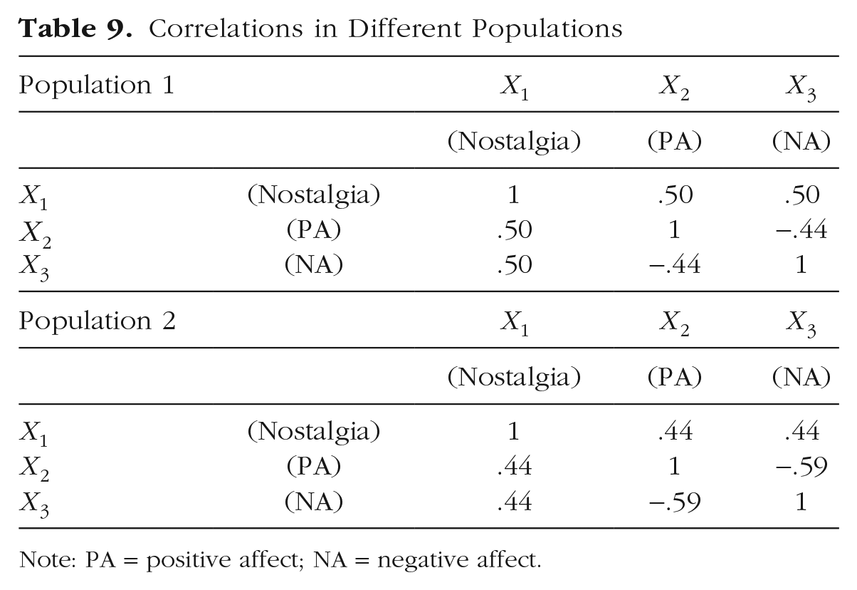
Note: PA = positive affect; NA = negative affect.

Obtaining good population estimates

Identifying accurate estimates of population-level correlations is, as evident from the above, a challenging endeavor. What are promising ways to do so? One potential source of effect sizes to be included in a proposed population correlation matrix is a meta-analysis. This analysis considers multiple studies simultaneously when estimating the size of an effect, which ought to improve the accuracy of the corresponding estimate. For example, the effect size assigned earlier to the impact of the gratitude intervention on well-being $(d = 0.17)$ is likely to be far more accurate than the effect size assigned to the correlation between boredom and gratitude ( $r = - . 25$ ) in the same section. After all, the former was derived from a large meta-analysis (Davis et al., 2016), whereas the latter was based on a single study (O’Dea et al., 2022).

Although “regular” meta-analyses can be a more accurate source of population effect-size estimations than single-study results, another promising and ambitious source of population effect-size estimates is meta-analytic structural equation modeling (MASEM; Becker, 1992, 1995; Cheung, 2013), which is an extension of multivariate meta-analysis (Becker, 2000). MAESM differs from regular meta-analysis in its capacity to perform meta-analyses on entire correlation matrices. Note that the individual studies that contribute to MASEM do not have to feature all variables in the correlation matrix in question but may contribute a part (Bergh et al., 2016). This is particularly useful for application in the detection of impossible hypotheses or effect-size limits for newly researched effects because studies that comprise the full set of relevant variables are unlikely to exist. In addition, MASEM allows researchers to include more specific relations between variables, such as mediation. The recent development of one-stage MASEM furthermore supports estimations of and corrections for heterogeneity across studies and allows the inclusion of categorical and continuous moderators to account for this (Jak & Cheung, 2020). To make this promising method more accessible for researchers, Jak et al. (2021) and Cheung (2015) developed practical guidance, an interactive web application, and a dedicated R package.

Note, however, that even meta-analyses are subject to sources of inaccuracy. Issues such as heterogeneity across studies, questionable research practices, publication bias, and selective reporting can all bias meta-analytic results (Ioannidis, 2008; Ones et al., 2017). In the attempt to gauge the accuracy of effect sizes obtained through meta-analysis in particular, researchers may turn to tools such as sensitivity analysis, the p-curve and p-uniform methods (Carter et al., 2019), and correcting for range restrictions in the data (Hunter et al., 2006). In a sensitivity analysis, the meta-analytic effect is compared across study subgroups (e.g., based on methodological differences or sample differences; Impellizzeri & Bizzini, 2012), and this can expose heterogeneity in study estimates. The p-curve and p-uniform methods can help find publication bias and, in the latter case, provide a bias-corrected effect-size estimate (Simonsohn et al., 2014; Van Aert et al., 2016). Range restrictions, in which variance is underestimated because of, for example, censored observations (Ree et al., 1994), can be remedied using procedures developed by Hunter et al. (2006) and validated by Le and Schmidt (2006).

Fortunately, current recommendations for meta-analysis in psychology tend to feature recommendations for the inclusion of such bias-detection measures (e.g., Carter et al., 2019; Johnson, 2021), making it easier for researchers to evaluate their accuracy. Nevertheless, when population estimates, derived from meta-analysis or otherwise, are rather uncertain, one may treat corresponding effect-size limits more as rough guide rather than an exact estimation.

Caveats

Psychological hypotheses are increasingly enriched with specific effect sizes. We called for and demonstrated above the importance of considering mathematical limits to effect sizes and whether their corresponding hypotheses might prove impossible. Within the predominantly multivariate populations that psychology considers, the maximum and minimum sizes that effects can take may be more restrictive then researchers might assume. This notion adds further nuance to the existing debate about what effect sizes are reasonable to expect. It aids researchers in interpreting measured effect sizes and enables them to predict limits on the possible correlations within populations. We wish to preempt a number of tentative misunderstandings about the work presented above, listed below.

First, it is important to underscore that the effect-size limits as computed in the current article refer to populations and not merely to specific samples. One of the implications of this is that whether or not a particular variable is part of one’s empirical sample is irrelevant to the limits of the size that an effect may take; what matters is if this variable features in the population. Thus, even if studies deal with a small number of focal variables, one may consider other variables in the population in estimating realistic effect sizes.

Second, our treatise of hypotheses and effect sizes has been applied only to cases of linear models with multivariate normal distributions. We suspect that the vast majority of psychological models are indeed linear and assume multivariate normality. However, our findings may not generalize readily to nonlinear models or variables that feature different distributions. Future work may look into these other settings.

A third word of caution is warranted about the role of null correlations. It may seem intuitively appealing to assume that a correlation between two variables of $r = . 0$ does not provide any restrictions on the correlations that these variables may have with others. After all, a null correlation implies that the two variables behave independently. However, as evident in Figure 3, in the context of three variables, a null correlation between two variables can prove impossible if these two variables each correlate strongly with others.

Fourth, we emphasize that our approach deals with whether or not hypotheses, in the form of correlation matrices, are possible and within what range an effect can be expected to fall. Our approach does not tell the researcher whether a hypothesis or effect-size range is also theoretically or practically important. The theoretical or practical importance of effect sizes is something that will depend, instead, on context (Busseri, 2018; Fritz et al., 2012; Giner-Sorolla et al., 2023).

Conclusion

It has become increasingly common in psychological science to accompany hypotheses with statements about the size that an effect may take, explicitly in the hypotheses themselves or in associated power analyses. Estimating such effect sizes a priori can be a challenge because they may vary across contexts, methodologies, and populations. Different from much recent work on this topic, we examined how one can be more accurate in hypothesizing effect sizes based on their statistical qualities. Effect sizes that pertain to variables within multivariate populations—as is common in psychology—may require a more restrictive size range than often assumed. Accordingly, it is important to consider the wider multivariate population context in which a hypothesis is made. By examining how other variables in the population (likely) relate to those that feature in the hypothesis, one can narrow down the limits between which the hypothesized effect may fall. This statistical triangulation process even works, and is perhaps particularly useful, if prior evidence for a hypothesised effect size is lacking—a typical scenario for novel hypotheses. Accordingly, estimating limits to effect sizes in the context of the broader multivariate population may help to prevent proposing impossible hypotheses and can give researchers a better idea of the size range in which their effects will reside.

Supplemental Material

sj-pdf-1-amp-10.1177_25152459231197605 – Supplemental material for Impossible Hypotheses and Effect-Size Limits

Supplemental material, sj-pdf-1-amp-10.1177_25152459231197605 for Impossible Hypotheses and Effect-Size Limits by Wijnand A. P. van Tilburg and Lennert J. A. van Tilburg in Advances in Methods and Practices in Psychological Science

Footnotes

Acknowledgements

We thank Paul H. P. Hanel, Reinhard Pekrun, and Nikhila Mahadevan for their helpful feedback on a draft of this article. For the purpose of Open Access, the authors have applied a CC BY public copyright license to any Author Accepted Manuscript (AAM) version arising from this submission. All authors consented to the submission of this manuscript.

Transparency

Action Editor: Jessica Kay Flake

Editor: David A. Sbarra

Author Contribution(s)

Wijnand A. P. van Tilburg: Conceptualization; Formal analysis; Investigation; Methodology; Project administration; Software; Validation; Visualization; Writing – original draft; Writing – review & editing.

Lennert J. A. van Tilburg: Conceptualization; Formal analysis; Investigation; Methodology; Project administration; Validation; Visualization; Writing – original draft; Writing – review & editing.

Correction (December 2023):

This article has been updated since its original publication; for further details please see .

ORCID iD

Wijnand A. P. van Tilburg

Supplemental Material

Additional supporting information can be found at

Notes

References

Abeyta

A. A.

Routledge

Kaslon

(2020). Combating loneliness with nostalgia: Nostalgic feelings attenuate negative thoughts and motivations associated with loneliness. Frontiers in Psychology, 11, Article 1219. https://doi.org/10.3389/fpsyg.2020.01219

Becker

B. J.

(1992). Using results from replicated studies to estimate linear models. Journal of Educational Statistics, 17(4), 341–362. https://doi.org/10.3102/107699860170043

Becker

B. J.

(1995). Corrections to “using results from replicated studies to estimate linear models.” Journal of Educational and Behavioral Statistics, 20(1), 100–102. https://doi.org/10.2307/1165390

Becker

B. J.

(2000). Multivariate meta-analysis. In Tinsley

H. E. A.

Brown

S. D.

(Eds.), Handbook of applied multivariate statistics and mathematical modeling (pp. 499–525). Academic Press.

Bergh

D. D.

Aguinis

Heavey

Ketchen

D. J.

Boyd

B. K.

Lau

C. L.

Joo

(2016). Using meta-analytic structural equation modeling to advance strategic management research: Guidelines and an empirical illustration via the strategic leadership-performance relationship. Strategic Management Journal, 37(3), 477–497. https://doi.org/10.1002/smj.2338

Busseri

M. A.

(2018). Examining the structure of subjective well-being through meta-analysis of the associations among positive affect, negative affect, and life satisfaction. Personality and Individual Differences, 122, 68–71. https://doi.org/10.1016/j.paid.2017.10.003

Carter

E. C.

Schönbrodt

F. D.

Gervais

W. M.

Hilgard

(2019). Correcting for bias in psychology: A comparison of meta-analytic methods. Advances in Methods and Practices in Psychological Science, 2(2), 115–144. https://doi.org/10.1177/2515245919847196

Cheung

M. W.-L.

(2013). Multivariate meta-analysis as structural equation models. Structural Equation Modeling: A Multidisciplinary Journal, 20(3), 429–454.

Cheung

M. W.-L.

(2015). Metasem: An r package for meta-analysis using structural equation modeling. Frontiers in Psychology, 5, Article 1521. https://doi.org/10.3389/fpsyg.2014.01521

10.

Cohen

(1988). Statistical power analysis for the behavioral sciences. Routledge. https://doi.org/10.4324/9780203771587

11.

Cohen

(2013). Statistical power analysis for the behavioral sciences. Academic Press. https://doi.org/10.4324/9780203771587

12.

Cooper

Findley

(1982). Expected effect sizes: Estimates for statistical power analysis in social psychology. Personality and Social Psychology Bulletin, 8(1), 168–173. https://doi.org/10.1177/014616728281026

13.

Cumming

(2013). Understanding the new statistics: Effect sizes, confidence intervals, and meta-analysis. Routledge. https://doi.org/10.4324/9780203807002

14.

Davis

D. E.

Choe

Meyers

Wade

Varjas

Gifford

Quinn

Hook

J. N.

Van Tongeren

D. R.

Griffin

B. J.

Worthington

E. L.

(2016). Thankful for the little things: A meta-analysis of gratitude interventions. Journal of Counseling Psychology, 63(1), 20–31. https://doi.org/10.1037/cou0000107

15.

Emmonse

Mccullough

M. E.

(2003). Counting blessings versus burdens: An experimental investigation of gratitude and subjective well-being in daily life. Journal of Personality and Social Psychology, 84(2), 377–389. https://doi.org/10.1037/0022-3514.84.2.377

16.

Fahlman

S. A.

Mercer-Lynn

K. B.

Flora

D. B.

Eastwood

J. D.

(2013). Development and validation of the multidimensional state boredom scale. Assessment, 20(1), 68–85. https://doi.org/10.1177/1073191111421303

17.

Fiedler

(2011). Voodoo correlations are everywhere—Not only in neuroscience. Perspectives on Psychological Science, 6(2), 163–171. https://doi.org/10.1177/1745691611400237

18.

Francis

Thunell

(2022). Data detective methods for revealing questionable research practices. In O’Donohue

Masuda

Lilienfeld

(Eds.), Avoiding questionable research practices in applied psychology (pp. 123–145). Springer. https://doi.org/10.1007/978-3-031-04968-2_6

19.

Fritz

C. O.

Morris

P. E.

Richler

J. J.

(2012). Effect size estimates: Current use, calculations, and interpretation. Journal of Experimental Psychology: General, 141(1), 2–18. https://doi.org/10.1037/a0024338

20.

Funder

D. C.

Ozer

D. J.

(2019). Evaluating effect size in psychological research: Sense and nonsense. Advances in Methods and Practices in Psychological Science, 2(2), 156–168. https://doi.org/10.1177/2515245919847202

21.

Gaertner

S. L.

Dovidio

J. F.

Anastasio

P. A.

Bachman

B. A.

Rust

M. C.

(1993). The common ingroup identity model: Recategorization and the reduction of intergroup bias. European Review of Social Psychology, 4(1), 1–26. https://doi.org/10.1080/14792779343000004

22.

Giner-Sorolla

Montoya

Aberson

Carpenter

Lewis

Jr. Bostyn

D. H.

Conrique

B. G.

B. W.

Schoemann

A. M.

Soderberg

C. K.

(2023). Power to detect what? Considerations for planning and evaluating sample size. PsyArXiv. https://doi.org/10.31234/osf.io/rv3kw

23.

Gniazdowski

(2013). Geometric interpretation of a correlation. Zeszyty Naukowe Warszawskiej Wyz.szej Szkoły Informatyki, 9(7), 27–35. https://doi.org/10.26348/znwwsi.9.27

24.

Greenwald

A. G.

Banaji

M. R.

Nosek

B. A.

(2015). Statistically small effects of the implicit association test can have societally large effects. Journal of Personality and Social Psychology, 108(4), 553–561. https://doi.org/10.1037/pspa0000016

25.

Hunter

J. E.

Schmidt

F. L.

(2006). Implications of direct and indirect range restriction for meta-analysis methods and findings. Journal of Applied Psychology, 91(3), 594–612. https://doi.org/10.1037/0021-9010.91.3.594

26.

Impellizzeri

F. M.

Bizzini

(2012). Systematic review and meta-analysis: A primer. International Journal of Sports Physical Therapy, 7(5), 493–503.

27.

Ioannidis

J. P.

(2008). Interpretation of tests of heterogeneity and bias in meta-analysis. Journal of Evaluation in Clinical Practice, 14(5), 951–957. https://doi.org/10.1111/j.1365-2753.2008.00986.x

28.

Jak

Cheung

M. W.-L.

(2020). Meta-analytic structural equation modeling with moderating effects on SEM parameters. Psychological Methods, 25(4), 430–455. https://doi.org/10.1080/10705511.2013.797827

29.

Jak

Kolbe

de Jonge

Cheung

M. W.-L.

(2021). Meta-analytic structural equation modeling made easy: A tutorial and web application for one-stage MASEM. Research Synthesis Methods, 12(5), 590–606. https://doi.org/10.1002/jrsm.1498

30.

Johnson

B. T.

(2021). Toward a more transparent, rigorous, and generative psychology. Psychological Bulletin, 147(1), 1–15. https://doi.org/10.1037/bul0000317

31.

Kong

Ding

Zhao

(2015). The relationships among gratitude, self-esteem, social support and life satisfaction among undergraduate students. Journal of Happiness Studies, 16(2), 477–489. https://doi.org/10.1007/s10902-014-9519-2

32.

Schmidt

F. L.

(2006). Correcting for indirect range restriction in meta-analysis: Testing a new meta-analytic procedure. Psychological Methods, 11(4), 416–438.

33.

Lorenzo-Seva

Ferrando

P. J.

(2021). Not positive definite correlation matrices in exploratory item factor analysis: Causes, consequences and a proposed solution. Structural Equation Modeling: A Multidisciplinary Journal, 28(1), 138–147. https://doi.org/10.1080/10705511.2020.1735393

34.

Marcus

Minc

(1988). Introduction to linear algebra. Courier Corporation.

35.

Neter

Kutner

M. H.

Nachtsheim

C. J.

Wasserman

, et al (1996). Applied linear statistical models. WCB McGraw-Hill.

36.

Neto

(2014). Psychometric analysis of the short-form UCLA Loneliness Scale (ULS-6) in older adults. European Journal of Ageing, 11(4), 313–319. https://doi.org/10.1007/s10433-014-0312-1

37.

O’Dea

M. K.

Igou

E. R.

Van Tilburg

W. A. P.

(2023). Preventing boredom with gratitude: The role of meaning in life [Manuscript submitted for publication].

38.

Ones

D. S.

Viswesvaran

Schmidt

F. L.

(2017). Realizing the full potential of psychometric meta-analysis for a cumulative science and practice of human resource management. Human Resource Management Review, 27(1), 201–215. https://doi.org/10.1016/j.hrmr.2016.09.011

39.

Ree

M. J.

Carretta

T. R.

Earles

J. A.

Albert

(1994). Sign changes when correcting for range restriction: A note on Pearson’s and Lawley’s selection formulas. Journal of Applied Psychology, 79(2), 298–301.

40.

Sawilowsky

S. S.

(2009). New effect size rules of thumb. Journal of Modern Applied Statistical Methods, 8(2), Article 26. https://doi.org/10.22237/jmasm/1257035100

41.

Sedikides

Wildschut

Arndt

Routledge

(2008). Nostalgia: Past, present, and future. Current Directions in Psychological Science, 17(5), 304–307. https://doi.org/10.1111/j.1467-8721.2008.00595.x

42.

Simonsohn

Nelson

L. D.

Simmons

J. P.

(2014). P-curve: A key to the file-drawer. Journal of Experimental Psychology: General, 143(2), 534–547. https://doi.org/10.1037/a0033242

43.

Sztachańska

Krejtz

Nezlek

J. B.

(2019). Using a gratitude intervention to improve the lives of women with breast cancer: A daily diary study. Frontiers in Psychology, 10, Article 1365. https://doi.org/10.3389/fpsyg.2019.01365

44.

Tajfel

(2010). Social identity and intergroup relations (Vol. 7). Cambridge University Press.

45.

Van Aert

R. C.

Wicherts

J. M.

van Assen

M. A

. (2016). Conducting meta-analyses based on p values: Reservations and recommendations for applying p-uniform and p-curve. Perspectives on Psychological Science, 11(5), 713–729. https://doi.org/10.1177/1745691616650874

46.

Van Tilburg

W. A. P.

Sedikides

Wildschut

. (2018). Adverse weather evokes nostalgia. Personality and Social Psychology Bulletin, 44(7), 984–995. https://doi.org/10.1177/0146167218756030

47.

Vul

Harris

Winkielman

Pashler

(2009). Puzzlingly high correlations in FMRI studies of emotion, personality, and social cognition. Perspectives on Psychological Science, 4(3), 274–290. https://doi.org/10.1111/j.1745-6924.2009.01125.x

48.

Wagenmakers

E.-J.

Love

Marsman

Jamil

Verhagen

Selker

Gronau

Q. F.

Dropmann

Boutin

Meerhoff

Knight

Raj

van Kesteren

E. J.

van Doorn

Šmíra

Epskamp

Etz

Matzke

. . . Morey

R. D.

(2018). Bayesian inference for psychology. Part II: Example applications with JASP. Psychonomic Bulletin & Review, 25(1), 58–76. https://doi.org/10.3758/s13423-017-1323-7

49.

Wildschut

Sedikides

(2020). The psychology of nostalgia: Delineating the emotion’s nature and functions. In Jacobsen

M. H.

(Ed.), Nostalgia now (pp. 47–65). Routledge.

50.

Zhou

Sedikides

Wildschut

Gao

D.-G.

(2008). Counteracting loneliness: On the restorative function of nostalgia. Psychological Science, 19(10), 1023–1029. https://doi.org/10.1111/j.1467-9280.2008.02194.x

51.

Zhou

Wildschut

Sedikides

Chen

Vingerhoets

A. J.

(2012). Heartwarming memories: Nostalgia maintains physiological comfort. Emotion, 12(4), 678–684. https://doi.org/10.1037/a0027236

Supplementary Material

Please find the following supplemental material available below.

For Open Access articles published under a Creative Commons License, all supplemental material carries the same license as the article it is associated with.

For non-Open Access articles published, all supplemental material carries a non-exclusive license, and permission requests for re-use of supplemental material or any part of supplemental material shall be sent directly to the copyright owner as specified in the copyright notice associated with the article.

0.00 MB

0.20 MB