Evaluating Effect Size in Psychological Research: Sense and Nonsense

Abstract

Effect sizes are underappreciated and often misinterpreted—the most common mistakes being to describe them in ways that are uninformative (e.g., using arbitrary standards) or misleading (e.g., squaring effect-size rs). We propose that effect sizes can be usefully evaluated by comparing them with well-understood benchmarks or by considering them in terms of concrete consequences. In that light, we conclude that when reliably estimated (a critical consideration), an effect-size r of .05 indicates an effect that is very small for the explanation of single events but potentially consequential in the not-very-long run, an effect-size r of .10 indicates an effect that is still small at the level of single events but potentially more ultimately consequential, an effect-size r of .20 indicates a medium effect that is of some explanatory and practical use even in the short run and therefore even more important, and an effect-size r of .30 indicates a large effect that is potentially powerful in both the short and the long run. A very large effect size (r = .40 or greater) in the context of psychological research is likely to be a gross overestimate that will rarely be found in a large sample or in a replication. Our goal is to help advance the treatment of effect sizes so that rather than being numbers that are ignored, reported without interpretation, or interpreted superficially or incorrectly, they become aspects of research reports that can better inform the application and theoretical development of psychological research.

Keywords

benchmarks correlation effect size evaluation

Nonsense: Words or language having no meaning or conveying no intelligible ideas

—Merriam-Webster (“Nonsense,” 2019)

Psychological research has a long tradition of evaluating findings according to whether they are statistically “significant” or not, but more recently, increasing attention has been paid to the size as opposed to the significance of effects (e.g., Cumming, 2012). Effect size refers to the magnitude of the relation between the independent and dependent variables, and it is separable from statistical significance, as a highly significant finding could correspond to a small effect, and vice versa, depending on the study’s sample size. Students are routinely taught how to calculate and interpret significance levels; they are less often taught how to calculate effect sizes, and even more rarely are they taught how to evaluate them. This neglect of effect size persists into the research careers of many psychologists.

Much of the published literature reflects this continued neglect. Although many journals now require that effect sizes be reported, and researchers (usually) dutifully follow this requirement, they often ignore effect sizes otherwise. When researchers do draw implications from effect sizes, the interpretations they offer are, more often than not, superficial, uninformative, misleading, or completely wrong. In sum, effect sizes are widely unappreciated and often misunderstood, even by professional researchers.

Current research on psychological methods (e.g., as published in Psychological Methods) has not been particularly helpful in this regard. Much of this work concerns the development, specification, and testing of ever more elaborate or precise quantitative models, and only occasionally does it address the concerns of substantive researchers grappling with the “solved” problem of reliably detecting and measuring simple bivariate effects. When such concerns do come to the fore, as in recent methodological articles and blog posts debating whether the threshold for rejecting the null hypothesis should be p < .05 or p < .005 (Benjamin et al., 2018), little reference is made to effect size. Despite exhortations to report effect sizes (e.g., Cumming, 2012), frank discussions of how to evaluate them remain surprisingly rare (but see Lakens, Scheel, & Isager, 2018). The purpose of the present article is to help to remedy this imbalance.

Effect Size

The two most commonly used measures of effect size are Cohen’s d and Pearson’s r. The former, typically used to characterize the differences in means between experimental groups, is the mean difference divided by the pooled standard deviation. The latter, the correlation coefficient, is typically used to characterize the degree to which one variable can be predicted from another. These two measures of effect size can be algebraically converted from one to the other; for simplicity and consistency, we focus on r in this article.

Although for a considerable period of psychology’s history it was common practice to report p levels in the absence of effect sizes, in recent years most journals have mandated that effect sizes be reported. For example, the publication manual of the American Psychological Association (2010), which is followed by many of the most visible outlets for psychological research, now states that reporting effect size is “almost always necessary” (2010, p. 34), and indeed, most (not all) articles in the association’s journals obediently report some effect-size measure, parenthetically, and usually alongside the p value. This mandated reporting is not always done enthusiastically. In a personal communication¹ with an author of this article, a prominent and widely published social psychologist wrote that

the key to our research [is not] to accurately estimate effect size. . . . When I am testing a theory about whether, say, positive mood reduces information processing in comparison with negative mood, I am worried about the direction of the effect, not the size. But if the results of such studies consistently produce a direction of effect where positive mood reduces processing in comparison with negative mood, I would not at all worry about whether the effect sizes are the same across studies or not, and I would not worry about the sheer size of the effects across studies. This is true in virtually all research settings in which I am engaged. I am not at all concerned about the effect size. (quoted in Funder, 2013, para. 4)

This is not an unusual opinion; similar comments can be found in a number of articles and blog posts. However, there are two problems with this line of thinking. First, and most obviously, this researcher routinely uses p levels to evaluate whether or not to be confident that a study has yielded a meaningful result. Given the study’s sample size, setting a threshold p level for accepting a result is exactly the same thing as setting a minimum effect size for the same decision. For example, in a two-group experimental study with 60 subjects, setting a two-tailed p threshold of .05 is equivalent to setting an r of .254 as the effect-size threshold. It is difficult to see how the first of these numbers could be worthy of “concern” if the second one is not. Second, and only slightly less obviously, the social psychological literature is filled with (usually nonnumerical) references to effect size, such as claims that certain manipulations can have “large” or even “surprisingly large” effects, or that (in the case of the fundamental attribution error) most people believe personality traits have “larger” effects than they really do. Such claims proceed in an empirical vacuum without some kind of quantitative measure of effect size.²

The Two Most Common Ways to Interpret Effect Size

Interpretation of effect sizes traditionally proceeds in one of two ways. The first is literally nonsensical (in the meaning expressed in the definition opening this article), and the other is seriously misleading.

Cohen’s standards

The nonsensical but widely used interpretation of effect size is the famous standard set by Jacob Cohen (1977, 1988), who set r values of .10, .30, and .50 as the thresholds for small, medium, and large effects, respectively. Cohen (1988) reluctantly used these conventions in the context of power analysis “only when no better basis . . . [was] available” (p. 25) and later told friends that he actually regretted having suggested them at all (R. Rosenthal, personal communication, November 2018). He had good reason for this regret. The terms small, medium, and large are meaningless in the absence of a frame of reference. They immediately require an answer to at least one of two questions: (a) small, medium, or large compared with what? and (b) small, medium, or large for what purpose? (We return to these questions later in this article.)

Squaring the correlation

As bad as these decontextualized criteria are, the other widely used way to evaluate effect size is arguably even worse. This method is to take the reported r and square it. For example, an r of .30, squared, yields the number .09 as the “proportion of variance explained,” and this conversion, when reported, often includes the word “only,” as in “the .30 correlation explained only 9% of the variance.”

We suggest that this calculation has become widespread for three reasons. First, it is easy arithmetic that gives the illusion of adding information to a statistic. Second, the common terminology of variance explained makes the number sound as if it does precisely what one would want to it do, the word explained evoking a particularly virtuous response. Third, the context in which this calculation is often deployed allows writers to disparage certain findings that they find incompatible with their own theoretical predilections. One prominent example is found in Mischel’s (1968) classic critique of personality psychology, in which he complained that the “personality coefficient” of .30, described by him as the highest correlation empirically found between trait measurements and behavior,³ “accounts for less than 10 percent of the relevant variance” (p. 38). As Abelson (1985) observed, “it is usually an effective criticism when one can highlight the explanatory weakness of an investigator’s pet variables in percentage terms” (p. 129).

The computation of variance involves squaring the deviations of a variable from its mean. However, squared deviations produce squared units that are less interpretable than raw units (e.g., squared conscientiousness units). As a consequence, r² is also less interpretable than r because it reflects the proportion of variance in one variable accounted for by another. One can search statistics textbook after textbook without finding any attempt to explain why (as opposed to assert that) r² is an appropriate effect-size measure. Although r² has some utility as a measure for model fit and model comparison, the original, unsquared r is the equivalent of a regression slope when both variables are standardized, and this slope is like a z score, in standard-deviation units instead of squared units.

Consider the difference in value between nickels and dimes. An example introduced by Darlington (1990) shows how this difference can be distorted by traditional analyses. Imagine a coin-tossing game in which one flips a nickel and then a dime, and receives a 5¢ or 10¢ payoff (respectively) if the coin comes up heads. From the payoff matrix in Table 1, correlations can be calculated between the nickel column and the payoff column (r = .4472) and between the dime column and the payoff column (r = .8944). If one squares these correlations to calculate the traditional percentage of variance explained, the result is that nickels explain exactly 20% of the variance in payoff, and dimes explain 80%. And indeed, these two numbers do sum neatly to 100%, which helps to explain the attractiveness of this method in certain analytic contexts. But if they lead to the conclusion that dimes matter 4 times as much as nickels, these numbers have obviously been misleading. The two rs afford a more informative comparison, as .8944 is exactly twice as much as .4472. Similarly, a correlation of .4 reveals an effect twice as large as a correlation of .2; moreover, half of a perfect association is .5, not .707 (Ozer, 1985, 2007). Squaring the r is not merely uninformative; for purposes of evaluating effect size, the practice is actively misleading.

Table 1.

Payoff Table for Darlington’s (1990) Example of a Coin-Tossing Game

Result of nickel toss	Result of dime toss	Total payoff
1	1	15¢
1	0	5¢
0	1	10¢
0	0	0¢

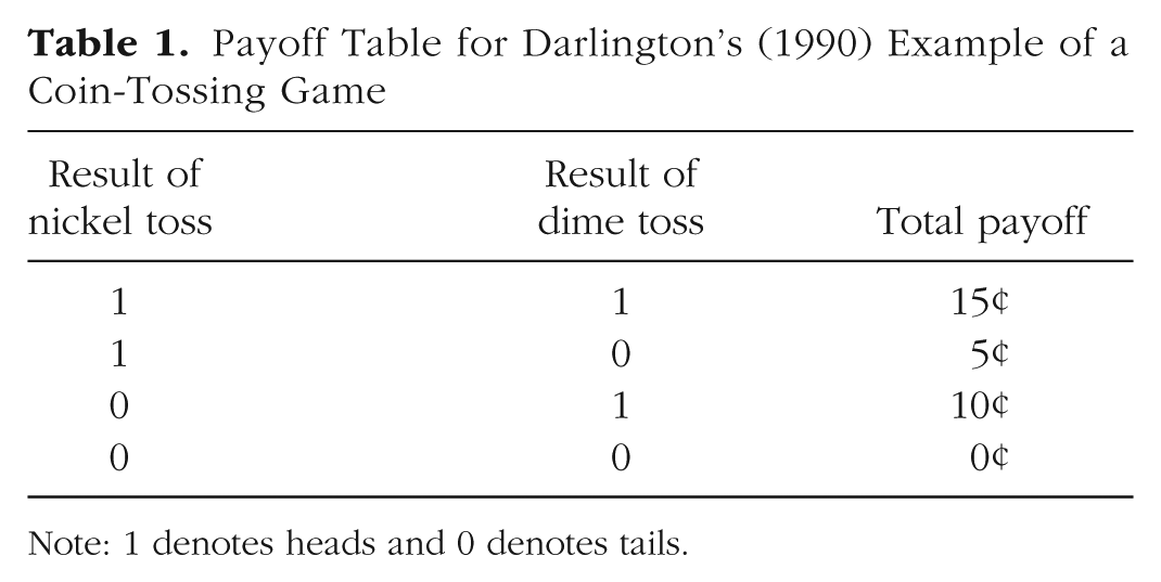
Note: 1 denotes heads and 0 denotes tails.

Toward Useful Interpretations of Effect Size

How can effect sizes be interpreted in a way that adds or provides meaning? We suggest two ways. The first is to use a benchmark, and the second is to estimate consequences.

Benchmarks

The idea behind using benchmarks to evaluate effect size is that the magnitude of a finding can be illuminated by comparing it with some other finding that is already well understood (or that at least is widely believed to be well understood). All of the benchmarking strategies we summarize in this section have the same aim: to help readers attain an intuitive “feel” for the meaning of an effect size. In the same way that people immediately gauge whether somebody is tall or short by comparing him or her with other people, researchers can approach a realistic appreciation of the meaning of a particular research result by using their knowledge of the sizes of classic findings, average findings, or other effects that are understood through everyday experience. J. Cohen (1988) used this strategy to justify his labeling numerical effect-size values as small, medium, and large. He likened a small effect to several specific effects, such as the mean height difference between 16- and 17-year-old girls. Medium effects were characterized as those “visible to the naked eye” (p. 26), though it seems he may have grossly overestimated the sensitivity of observers to at least some characteristics (Ozer, 1993). Large effects were described as similar in magnitude to the difference in mean IQ between college graduates and people with just a 50-50 chance of graduating from high school. One might well quibble with Cohen’s choices of examples, but given that this was early work when few researchers were talking about effect size, it would seem more fruitful to consider other benchmarking approaches.

Classic studies

One example of the benchmarking approach is provided by an analysis we reported some years ago (Funder & Ozer, 1983). We performed a simple reanalysis of three classic findings in the psychological literature: Festinger and Carlsmith’s (1959) finding of a reverse effect of incentives on attitude change, Darley and Latané’s (1968) and Darley and Batson’s (1967) studies of bystander intervention, and Milgram’s (1975) demonstrations of experimentally induced obedience. In each case, from the reported findings we simply computed an effect-size r that reflected the degree to which the dependent variable (attitude change, helping, and obedience, respectively) was affected by the manipulated independent variable (incentive, hurry and number of bystanders, and distance between the experimenter and victim, respectively). In each case, the resulting r fell between .36 and .42.

This result should not have been surprising, but it was, in a zeitgeist in which a common complaint was that personality traits were not meaningfully related to behavioral outcomes because the correlations between them seldom exceeded .40 (e.g., Nisbett, 1980). And some writers at the time misinterpreted the implication of our calculations, in our view, by concluding that the calculations implied that these studies also “only” found “small” effects after all (or more disastrously, that “situations aren’t important either”). Our own view was that these studies were and remain classics of the social psychological literature, and nobody, certainly nobody at the time, doubted that the effects reported were foundation stones of social psychology that should be taught to every student in that field. We simply thought it was worth knowing that the reported effect sizes were in roughly the same range as the purported ceiling for effects of personality.

Other well-established psychological findings

In a later, similar, but much broader set of reanalyses, Richard, Bond, and Stokes-Zoota (2003) also calculated the effect-size rs for well-established findings in psychology. To list a few examples, scarcity increases the perceived value of a commodity (r = .12), people attribute failures to bad luck (r = .10), communicators perceived as more credible are more persuasive (r = .10), and people in a bad mood are more aggressive than those in a good mood (r = .41). One is free to decide whether or not to interpret any of these findings as reliable or important, but to the extent that one does, the associated effect sizes provide a useful benchmark for interpreting other findings in the literature.

A similar analysis was performed by Roberts, Kuncel, Shiner, Caspi, and Goldberg (2007), who compared the validity of personality traits for predicting mortality, divorce, and occupational success with the well-established validity of socioeconomic status and intelligence as predictors of these same outcomes. The result was that the “magnitude of the effects . . . was indistinguishable” (p. 313). Even more striking, perhaps, was that for the prediction of mortality, the estimated rs for all the predictors ranged no higher than .24 and for the most part fell below .10.

Comparisons with “all” studies

In even broader efforts, researchers have provided potential effect-size benchmarks by computing averages based on comprehensive reviews of the social and personality psychology literatures. In their ambitious effort, Richard et al. (2003) also calculated an average effect size for all the published effects in the social psychological literature that they were able to survey, and the resulting value was .21. A parallel but less extensive project surveyed the personality literature and came up with precisely the same average effect size: r = .21 (Fraley & Marks, 2007). Of course, both of these results are very likely to be overestimates of the true effects of the variables studied, because of publication bias that privileges significant findings (and so, on average, larger effects). Therefore, a researcher who obtains an r of .21 in a new study can be fairly confident that this is a larger effect than typically found.

A more recent and very large project reviewed 708 meta-analytically derived correlations from the literatures of both social and personality psychology, and found that the average effect-size r was .19, and that rs of .11 and .29 fell at the 25th and 75th percentiles, respectively (Gignac & Szodorai, 2016). The authors suggested recasting Cohen’s guidelines in this light, such that correlations of .10, .20, and .30 could be considered small, typical, and relatively large, respectively (p. 74).

Comparisons with intuitively understood nonpsychological relations

Ordinary life experience or broader reading can lead to a sense of the strength of relationship between variables, and this understanding can also be used as an aid to the intuitive appreciation of a research finding. For example, do you take antihistamines to combat a runny nose and sneezing? If so, how well do they work? According to one estimate, the effect size of the relationship between antihistamine use and relief from these symptoms is equivalent an r of .11. Do you take a pain reliever to alleviate headaches? The relieving effect of nonsteroidal anti-inflammatory drugs (such as ibuprofen) on pain is not much different from the effectiveness of antihistamines on sneezing, r = .14. Other familiar benchmarks for intuitively calibrating effects include the tendency of men to weigh more than women (r = .26), the tendency of places at higher elevations to have lower average annual temperatures (r = −.34), and the correlation between height and weight for U.S. adults (r = .44). And a really big one: The effect size of the average height difference between men and women is equivalent to an r of .67 (all these findings are summarized by Meyer et al., 2001, pp. 131–132).

Consequences

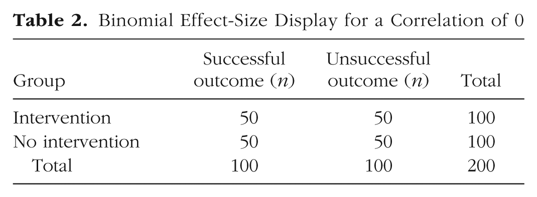
The binomial effect-size display

A more direct way to evaluate an effect size is to consider consequences, which in some cases can be numerically calculated. Perhaps the best known and easiest to use of these methods is the binominal effect-size display (BESD), introduced by Rosenthal and Rubin (1982). The BESD illustrates the size of an effect, reported in terms of r, using a 2 × 2 table of outcomes. In its usual application, the process begins with assuming that a sample of 200 individuals has been divided into two equal-sized groups, one of which has experienced an intervention (e.g., a drug for a disease all 200 have) and one of which has not. It is further assumed, for the sake of illustration, that for half the individuals the intervention was successful, and for the other half it was not. If the intervention (or drug) had no effect at all (r = 0), the 2 × 2 table would look like Table 2. In Rosenthal and Rubin’s favorite (hypothetical) example, the intervention comprises giving a drug or not, and the outcome is being alive or dead at the end of the study, but the method can be applied more generally in less dramatic scenarios; any pairing of a dichotomous predictor and dichotomous outcome can be analyzed in this way. The effect-size r can easily be incorporated in a BESD table by multiplying it by 100 (to remove the decimal), dividing it by 2, adding 50, and placing the result in the upper left-hand corner. The remaining cells can then be determined by subtraction (because this table has 1 degree of freedom). If r is .30, the number in the upper left-hand corner is 65 (30/2 + 50 = 65), and the table looks like Table 3.

Table 2.

Binomial Effect-Size Display for a Correlation of 0

Group	Successful outcome (n)	Unsuccessful outcome (n)	Total
Intervention	50	50	100
No intervention	50	50	100
Total	100	100	200

Table 3.

Binomial Effect-Size Display for a Correlation of .30

Group	Successful outcome (n)	Unsuccessful outcome (n)	Total
Intervention	65	35	100
No intervention	35	65	100
Total	100	100	200

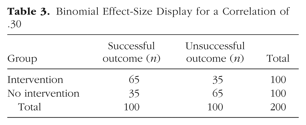
Some readers, traditionally trained to think of .30 correlations as “explaining only 9% of the variance” might be surprised to learn that an effect of this size will yield almost twice as many correct predictions as incorrect ones. More specifically, a table such as this, when combined with cost data for interventions and outcomes, could be used to calculate the utility of an intervention or of a predictive instrument in concrete, monetary terms. It could also be used, as in Rosenthal and Rubin’s (1982) own example, to assess the number of lives that could be saved by a health intervention. In a later analysis, Rosenthal (1990) calculated that the correlation of .03 between taking aspirin after a heart attack and prevention of future heart attacks implied the prevention of 85 attacks in a sample of 10,845 individuals. Less dramatically, a BESD could be used to calculate the payoff from using an ability or personality test to select employees. In a similar manner, the Taylor-Russell tables (Taylor & Russell, 1939) have long been used by industrial psychologists to combine the validity of a selection instrument with the selection ratio (the proportion of applicants hired) to predict the percentage of hired employees who will be successful on the job.⁴

Consequences in the long run

In a classic analysis (which is nonetheless not as widely known as it should be) subtitled “When a Little Is a Lot,” the well-known cognitive psychologist Robert Abelson (1985) calculated the correlation between a Major League baseball player’s outcome in a single at bat and his overall batting average. Abelson’s calculation yielded an r of .056,⁵ and he was so surprised by this result that he exclaimed (in print), “What’s going on here?” (p. 131). It is testimony to the degree to which the ritual of explaining variance had become mindlessly entrenched even in the thinking of sophisticated researchers that Abelson confessed that his “first reaction to this result [was] incredulity. . . . My personal intuition was jarred by this result, which seems much too small” (p. 131). The mystery appeared to deepen when he observed that almost all Major League baseball players have season averages within a limited range, between about .200 and .300.

However, the resolution to what Abelson characterized as a “paradox” (p. 131) turned out to be rather simple. The typical Major League baseball player has about 550 at bats in a season, and the consequences cumulate. This cumulation is enough, it seems, to drive the outcome that a team staffed with players who have .300 batting averages is likely on the way to the playoffs, and one staffed with players who have .200 batting averages is at risk of coming in last place. The salary difference between a .200 batter and a .300 batter is in the millions of dollars for good reason.

Another example comes from a large study that tracked 2 million financial transactions across more than 2,000 people. The correlation between an individual’s extraversion score and the amount he or she spent on holiday shopping was .09 (Weston, Gladstone, Graham, Mroczek, & Condon, 2018). Although this fact might not be very consequential for a single individual, multiply the effect by the number of people in a department store the week before Christmas, and it becomes obvious why merchandisers should care deeply about the personalities of their customers.

The overall implication, as Abelson (1985) noted, is that seemingly small effects can matter “in the long run, albeit not very consequentially in the single episode” (p. 133). In particular, a psychological process that affects the behavior of a single individual repeatedly⁶ over time, or, analogously, the behavior of many individuals simultaneously on a single occasion, can have hugely important implications.

Relevance for Psychological Research

Abelson’s (1985) illustration of how seemingly small effects can cumulate has important implications for psychology. Every social encounter, behavior, reaction, and feeling a person has could be considered a psychological “at bat.” And imagine how many of those occur in a day, a week, a year, or a lifetime—certainly many more than the 550 or so a ball player gets in a year. Any psychological variable that affects any of these, every time it happens, will have an effect that could cumulate over time, with important consequences for numerous life outcomes, including (to name just a few examples) popularity and social success, physical health, financial success, personal relationships, and overall quality of life.⁷

Individual differences research

The relevance of the cumulation of small effects over time is particularly obvious for research on individual differences, such as abilities or personality traits. If a stable trait—such as extraversion, agreeableness, or conscientiousness—affects much of what you do even in a small way, its consequences can add up very, and perhaps surprisingly, quickly. Analyses of the effects of personality on life outcomes have focused on long-term consequences such as health, relationship success, quality of life, and—that ultimate long-term consequence—longevity (Friedman et al., 1993; Ozer & Benet-Martínez, 2006; Roberts et al., 2007). But Abelson’s (1985) analysis suggests that one might need much less than a lifetime for noticeable consequences of stable personality traits to appear. A correlation of about .05 translates to large consequences with 550 at bats. How long does it take for a person to experience, for example, 550 interpersonal encounters?

Consider a student moving away from home to college and meeting the fellow residents of his dormitory for the first time. Assume that he is highly agreeable. How long will it take before he finds himself enjoying the enhanced popularity that is the reliable long-term result of this trait (Ozer & Benet-Martínez, 2006)? A back-of-the envelope calculation suggests that if the correlation between agreeableness and an individually successful social interaction is .05 (which is a hypothetical, conservative estimate⁸), and if the student has 20 social interactions a day, then the consequences for his popularity in less than a month (550 interactions/20 interactions per day = 27.5 days) will be as noticeable as the consequences of batting ability for a baseball player’s success at the end of the season.

Even more remarkably, Epstein (1979) demonstrated that broad outcome criteria could be predicted with surprising precision from broad, aggregated predictor variables. For example, he showed that a person’s average behavior over a period of 14 days could be predicted by the person’s average behavior over a preceding period of 14 days with a correlation equivalent to .80 to .90 (p. 1123). The moral of his demonstration is that an appropriate and realistic target for behavioral prediction is not what a person does on one day or in one situation, but what he or she does in the not-very-long run.

Experimental research

The relevance of the way effects can cumulate over time is perhaps less obvious for experimental research in which independent variables are manipulated, but it is fundamentally no different. If a psychological process is experimentally demonstrated, and this process is found to appear reliably, then its influence could in many cases be expected to accumulate into important implications over time or across people even if its effect size is seemingly small in any particular instance.

For example, a process that has a small influence on the degree to which a person can accomplish self-control every time he or she experiences fatigue—which is perhaps not every day, but certainly not rare—will be psychologically important for understanding what goes on when people are tired.⁹ Or, for another example, consider the recent conclusion that a meta-analytic r value of .08 indicates that a growth mind-set intervention has a “weak” effect on students’ achievement (Sisk, Burgoyne, Sun, Butler, & Macnamara, 2018, p. 549). This effect can be calculated to imply an average increase in grade point average (on the traditional 4-point scale) of 0.1 point, which when aggregated across all the students in a class, a school, or a school district could translate to a considerable increase in students’ achievement (Dweck, 2018; Gelman, 2018).¹⁰ Or, for a final example, consider an aspect of communication that (reliably) makes it even a tiny bit more persuasive. Such a factor may become important when a communication is conveyed to millions of people. Imagine, for example, that a political consultant is purchasing time for a TV ad that will be seen by 30 million viewers and is choosing between two possibilities that experimental research has shown differ in their effectiveness with an effect-size r of .05. The choice is obviously consequential. This is the sense in which experimentally demonstrated phenomena could cumulate in their importance even if their one-time (or one-person) effect sizes are in the range traditionally dismissed as weak.

A long-standing tradition in experimental social psychology has been to try to re-create real-world situations in the laboratory (Aronson & Carlsmith, 1968). Influential studies have simulated circumstances in which a person appears to be in distress, in order to assess the conditions under which a bystander might intervene; in which a person is given dire orders to harm another person, in order the assess the conditions under which obedience or disobedience becomes more likely; and in which a person is given an initial (false) impression of someone he or she is about to meet, in order to assess the conditions under which this impression becomes self-fulfilling. Such research has become increasingly rare in recent years, perhaps because it is difficult to conduct for operational and ethical reasons, and also because easier methods of research, such as gathering responses to computer-presented stimuli, have become widely available (Baumeister, Vohs, & Funder, 2007).

Indeed, to capture a meaningful aspect of social experience in a psychological laboratory, for even a few minutes, is a remarkably ambitious and even daunting goal. Some experimental findings from research of this sort turn out not to be replicable and thus are not reliable after all. But when some aspect of a situation does turn out to affect behavior, and the finding is reliable across experimental attempts and different laboratories, then lightning has been caught in a bottle,¹¹ and it is not wise or even realistic to demand a “large” effect size (Gelman, 2018). Under the circumstances, to find anything at all can be impressive (Prentice & Miller, 1992).

When effects do (and do not) cumulate

The foregoing discussion applies to circumstances in which the effects measured in a research study can be expected to cumulate over time, situations, or individuals. Small effects accumulate into large ones in at least some, and probably many, but certainly not all circumstances. This cumulation can occur across time and occasions for a given individual, and across individuals at a single time or occasion.

The batting average in baseball provides an unambiguous example of an effect that cumulates across time and situations for an individual. Hits add up (in the not-very-long run) into runs, and runs add up (also in the not-very-long run) into won games. Another example of cumulation that seems almost as clear to us is the way the (even slightly) larger probability of a friendly act by a more agreeable person can lead, before too long, to an enhanced social reputation. More generally, precisely because they are consistent over time and across situations, the influences of personality on behavior can confidently be expected to affect consequential social, occupational, and health outcomes, and in fact they do (Ozer & Benet-Martínez, 2006).

Not all cases are as clear-cut as these, however. It is not difficult to think of examples in which the consequences of repeated effects fail to increase, increase nonlinearly, or even reverse over time and occasions. The well-known Weber-Fechner and Yerkes-Dodson principles describe how responses to increases in the level of a stimulus or motivation tend to level off or even reverse; the principle of habituation posits that responses to a repeated stimulus will eventually cease altogether. Cognitive systems of emotion regulation and physiological systems that support homeostasis, similarly, can reduce or eliminate the effect of repeated stimuli. Another potential complication in interpreting cumulation is the Matthew effect, which suggests that the accumulation of advantages (or other consequences) from a psychological process can actually accelerate, perhaps differently over time for different individuals.

Even in cases in which the strength of an effect itself does not build steadily over time, however, the consequences of the underlying process still might. In the case of ego depletion, for example, imagine a person who dislikes her job so much that she comes home every evening in a state of psychological fatigue that makes her more likely (r = .05) to have a short fuse in stressful conversations with her spouse. Even if recovery processes repair the deficit in self-control by the next morning (e.g., Inzlicht & Schmeichel, 2012), the slightly increased daily probability of marital friction would seem likely to have important consequences in the medium run (say, about 2 years, or nearly 550 work days). And, on a theoretical level, an underlying process that can affect interpersonal interactions with a small but real probability on each individual occasion can be important for understanding relationships and many other outcomes that are the long-term result of many interactions.

As one thinks through examples such as these—and whether or not one agrees with any particular interpretation—a common gap in psychological theorizing becomes evident: Theorizing typically does not extend to considerations of when and in what ways individual differences, situational variables, and their underlying processes—which may have small effects on single occasions—can be expected to cumulate in their strength or consequences. Nor does theorizing commonly consider which sorts of processes will not cumulate in their strength or consequences. When and if psychological theorizing begins to take more careful account of effect sizes—one hoped-for goal of this article—attention to these questions will become critical. The metaphor of the psychological at bat may apply in many cases, but surely not all, and theories could be more helpful than they currently are in identifying them.

Reliable Estimation of Effect Sizes

Our analysis is based on a presumption that the effect size in question is, in fact, reliably estimated. This is a big presumption, and a critical concern when the effect size is in the range traditionally regarded as small. Although the difference between rs of .30 and .40 might not be terribly important for most theoretical or practical purposes, the difference between rs of .00 and .10 surely is. In that light, it is sobering to observe that the 95% confidence interval for an r of .10 will not quite exclude a value of .00 when the sample size is 400, and that excluding .00 from the 95% confidence interval for an r of .05 requires a sample size of 1,500. Fortunately, there are other ways to establish effect sizes besides relying on single studies with very large sample sizes. Meta-analytically, a series of diverse studies of a topic that all yield effect sizes within a narrow range (and in the same direction), even if the average effect is considered small, can provide some reasonable degree of confidence that the effect has been usefully estimated. In any event, it is clear that the precision of the estimate of the effect size becomes more important the smaller the effect size is.

Other, nonstatistical considerations can be of concern as well. Smaller effects are more at risk of being the product of an artifact rather than the process under investigation. For example, experimenter expectancy effects (Rosenthal, 1996), even if less powerful and more subtle than initially reported (Jussim, 2017), might be enough to account for effects in the range of, for example, the .08 effect of growth mind-set interventions we mentioned earlier . This example illustrates another facet of precise estimation when effects are small: Not only are larger sample sizes and more studies desirable, but also care in eliminating potential confounding variables becomes critically important. Other practices to reduce bias in analysis and reporting of research findings, such as preregistration of studies and the Registered Report process, can also be helpful, because the importance of potential bias becomes larger when effects or sample sizes are smaller.

Implications for Interpreting Research Findings

Our analysis of the evaluation of effect sizes has three important implications for how research findings should be interpreted.

Researchers should not automatically dismiss “small” effects

One reason why experimental social psychologists, in particular, have seemed reluctant to report or to emphasize effect sizes might be that, because of their traditional training (which often includes squaring correlations to yield the percentage of variance explained), they are taken aback by how small they seem. If readers of the psychological literature better understood the implications of effect size, apologies for reported effect sizes may no longer be necessary. An incentive structure that rewards performing selective analyses (p-hacking) in order to increase small effect sizes so they cross the threshold of statistical significance might be replaced by incentives that instead reward gathering data from large samples and unapologetically reporting small, effect sizes that are precise and reliable—which is no small accomplishment.

Indeed, researchers sometimes object to recommendations to gather data from large samples because they are concerned that small, unimportant effects will become significant. We believe this objection is mistaken, because it is smaller effect sizes that (realistically) will turn out to be the ones that are more likely to have been correctly estimated, and other things being equal, larger sample sizes are likely to provide more precise estimates regardless of the size of the effect.

Effect sizes will become more prominently and less reluctantly reported in experimental research, we believe, when researchers stop feeling (or being made to feel) defensive about them, and when explicit (rather than ritualized) discussions of the theoretical and practical implications of obtained effect sizes, of any magnitude, become more common. As publications with effect sizes reported in abstracts and perhaps even titles begin to accumulate in the literature, readers will begin to develop their own experientially based and more realistic intuitions about what small and large really mean in the context of psychological research.

Researchers should be more skeptical about “large” effects

On the flip side, the traditional neglect of effect-size reporting has also allowed some implausibly large effects to sneak in under the radar. One famous example is the reported effect of unscrambling words referring to stereotypes of the elderly on walking speed. In two studies (each with an N of 30), this task slowed walking speed with an effect size equivalent to .48 and .38, respectively (Bargh, Chen, & Burrows, 1996). These r values were not reported in the original article but are easily calculated from the reported t statistics. If they had been reported, and appropriately evaluated in terms of benchmarks, questions might have been raised about the plausibility of this effect really being about as large as the correlation between height and weight in U.S. adults (r = .44, as cited earlier; Meyer et al., 2001).¹²

Researchers have often reported anomalously large effect sizes in small-N studies. This might have been a sign, if heeded, that their overall reliability was not to be trusted. Because the confidence intervals of effect sizes in small studies are very wide, such studies can be expected to sometimes produce large apparent effects that replication studies reveal to be greatly overestimated (Cumming, 2012). A recent major project found that even for studies that were published in highly prestigious journals and whose findings could be successfully replicated, the replication effect sizes were about half the size of the originals (Camerer et al., 2018). In our view, enough experience has already accumulated to make one suspect that small effect sizes from large-N studies are the most likely to reflect the true state of nature.

Researchers should be more realistic about the aim of their programs of psychological research

Looking across a room full of research psychologists at a professional meeting, it is possible to be struck by the thought that everyone there believes, usually with some justification, that what he or she is studying is important. As a result, every psychologist is prone to expect that the variable he or she is studying should have a large effect on cognition, emotion, or behavior. This is perhaps sometimes true, but every researcher should also be aware that the psychologist in the next chair may be studying a very different topic with the same expectation. We all must face the fact: Human psychology is inherently complex, and there is only so much variation—in cognition, emotion, or behavior—to go around (Ahadi & Diener, 1989; De Boeck & Jeon, 2018).

How realistic is it to expect that any one research program, on any one topic or psychological process, determines more than a small piece of what is really going on in the psychological world at large? Perhaps all researchers should lower their expectations a little (or a lot). Psychologists are in the business of predicting the results of experiential or behavioral at bats and should not be surprised or begrudge that the variables they are studying must share their predictive validity with other correlates and causes.

Recommendations for Research Practice

Report effect sizes, always and prominently

The effect sizes for every study should be reported prominently. This is routine in individual differences articles, in which Pearson’s r is ubiquitous, but even these articles could more strongly emphasize the actual effect sizes, beyond the existence of the relationships reported. Reports on experimental research have farther to go; the effect sizes that are mandated to be reported should not be buried in Results sections, reluctantly mentioned between parentheses, but should be included in abstracts and Discussion sections as well. Over time, a base of experience will accumulate as readers of the literature—researchers and students alike—become gradually familiar with the effect sizes that are actually found in well-conducted research. A corollary of this recommendation is that the sample size of every study should be sufficient for the effect-size estimate to be at least somewhat reliable.

A recent example illustrating these recommendations is an article reporting a meta-analysis of 761 effect sizes, calculated with data gathered on a total sample of 420,595 (Allen & Walter, 2018). The article reported—in its abstract—several relationships between personality traits and sexual behavior, including (among others) correlations between extraversion and frequency of sexual activity (r = .17), agreeableness and sexually aggressive behavior (r = −.20), and conscientiousness and sexual infidelity (r = −.17). This is exactly the kind of reporting that not only illuminates the specific findings summarized, but also helps to build a larger understanding of how big important effects can really be expected to be.

Conduct studies with large samples (when possible)

As we have noted, an often-neglected complication in interpreting effect sizes is that the confidence interval of r is very wide with small samples. Schönbrodt and Perugini (2013) ran a series of Monte Carlo simulations that led them to conclude that “in typical scenarios sample size should approach 250 for stable estimates” (p. 609).

We believe that the effect size is information that should be reported and evaluated regardless of a study’s sample size. But the confidence interval should be reported as well, so that evaluation can be informed by the necessary degree of uncertainty when the sample size is small. The ideal solution is to run studies with large samples. This is not always feasible with certain kinds of research or subject populations (Finkel, Eastwick, & Reis, 2017). But an important priority should be to make samples as large as resources allow, and perhaps it would be wise to reallocate resources from numerous smaller studies to fewer larger ones. A few studies with larger samples are likely to produce more accurate and less confusing findings than will many studies with smaller samples. In particular, the recent history of social psychology illustrates the bewildering welter of seemingly contradictory results that can emerge from a literature dominated by small-N studies.

Report effect sizes in terms that are meaningful in context

Pearson’s r, emphasized in this article, is a standardized measure of effect size, which means it has no reference to, and provides no information about, the units of measurement used in the study. An insufficiently recognized property of standardized measures of effect size, such as r, is that they confound the consistency of an effect with the size of the effect. Imagine predicting annual salary from years of education in a heterogeneous sample of adults. It is possible, however fanciful, that the correlation between years of education and income is nearly 1.0, yet a year of education might be worth only a dollar in annual income: All cases might fall on a nearly flat regression line. In this scenario, the linear model fits the data very well, so the correlation is large, but the effect is very small, as would be shown by the raw regression coefficient. Or consider the opposite discrepancy between model fit and effect size: On average, education could have a very large effect on income (steep slope), but this effect could be highly variable (large standard error of estimate). In short, the fit of the linear model (the consistency of the effect) and the slope of the regression line (the size of the effect) are inherently confounded in standardized measures of effect size.

We are not the first to make the point that more meaningful measures of variables would lead to more meaningful measures of their effects (see, e.g., P. Cohen, Cohen, Aiken, & West, 1999). The need to employ standardized measures of effect size arises from the use of arbitrary and intrinsically meaningless measurement units. Researchers would be well served to be explicit about their measurement units and to utilize raw effect-size measures, such as mean differences or raw regression coefficients, alongside standardized measures of effect size, when possible. This would be a reminder of the ambiguities inherent to the standardized effect measures and would contribute toward the development of an interpretive framework for the most frequently used measurement units (Pek & Flora, 2018). With experience, even the meaning of a unit on a 7-point Likert scale might eventually become clear.

Moreover, in some cases, especially in applied research, the unit of measurement does have an intrinsic meaning. For example, mean differences in a countable health outcome, such as heart attacks, are meaningful in their own right and should be reported in preference to standardized measures, such as correlations or relative risks. The Harding Center for Risk Literacy (2018b), for instance, uses “fact boxes” to describe costs and benefits of health interventions in terms of concrete numbers, such as the number of people who would benefit from or be harmed by a screening or a drug. One of their fact boxes translates medical effect-size statistics in the following manner: Consider a sample of 200 people with acute bronchitis. If 100 of these people are given no treatment or a placebo, after 14 days 51 of them will still have a cough and 19 will feel ill in other ways (e.g., nausea). If the other 100 are given an antibiotic, 14 days later only 32 of them will still have a cough but 23 will feel ill otherwise (Harding Center for Risk Literacy, 2018a). This kind of format for presenting research results translates effect sizes into consequences people care about and use to make decisions.

Stop using empty terminology

It is far past time for psychologists to stop squaring rs so they can belittle the seemingly small percentage of variance explained and to stop mindlessly using J. Cohen’s (1977, 1988) guidelines, which even Cohen came to disavow. Ideally, words such as small and large would be expunged from the vocabulary of effect sizes entirely, because they are subjective and often arbitrary labels that add no information to results that can be reported quantitatively. This goal is probably unrealistic; indeed, in this article we have been unable to avoid the liberal use of these descriptive adjectives ourselves. But at the very least, it would be good to become in the habit of responding to characterizations of effect sizes as being small or large with questions about the implied comparison: The effects are small or large compared with what? Compared with what is usually found, with what other studies have shown, or with what it is useful to know? Or is another standard altogether being used? Whatever the standard of evaluation is, there ought to be one.

Revise the Cohen guidelines

This is our most presumptuous recommendation, and we offer it somewhat tongue in cheek, but not entirely. It is abundantly clear that the traditional Cohen guidelines (J. Cohen, 1977, 1988) are much too stringent. And as did Cohen, we think decontextualized guidelines are appropriate only for the most approximate of uses. But new guidelines can be proffered in the light of (a) Abelson’s (1985) demonstration of the not-so-long-term consequences of an effect-size r of .05, (b) the illustration, through a BESD, of how a correlation in the range of .30 can almost double predictive validity beyond chance, (c) the average sizes of effects in the published literature of social and personality psychology, and (d) the sizes of other relationships encountered in daily experience, such as the effectiveness of antihistamines or the association between height and weight.

We offer, therefore, the following New Guidelines: Assuming that estimates are reliable (a critical concern, as already discussed), an effect-size r of .05 indicates an effect that is very small for the explanation of single events but potentially consequential in the not-very-long run, an effect-size r of .10 indicates an effect that is still small at the level of single events but potentially more ultimately consequential, an effect-size r of .20 indicates an effect of medium size that is of some explanatory and practical use even in the short run and therefore even more important, and an effect-size r of .30 indicates an effect that is large and potentially powerful in both the short and the long run.¹³ A very large effect size (r = .40 or greater) in the context of psychological research is, we suggest, likely to be a gross overestimate that will rarely be found in a large sample or in a replication. Smaller effect sizes are not merely worth taking seriously. They are also more believable.

Summary and Conclusion

We began by describing problems with the traditional evaluation of effect sizes, including common ways in which they are misinterpreted—the most common mistake being to describe them in ways that either convey no useful information or are actively misleading. Next, we outlined several ways (building on proposals by prior writers) to imbue effect-size numbers with meaning. We concluded by offering some recommendations for the most useful ways to evaluate effect size and even, daringly, suggested a new set of standards. Our hope is that this article might play a small role in helping to advance the treatment of effect sizes so that rather than being numbers that are reported without interpretation, or interpreted superficially or incorrectly, they become aspects of research reports that will inform the application and theoretical development of psychological research.

Footnotes

Acknowledgements

We thank Ulrich Schimmack for identifying a calculation error in an earlier version of this manuscript.

Action Editor

Alexa Tullett served as action editor for this article.

Author Contributions

D. C. Funder and D. J. Ozer jointly generated the ideas for this article and jointly wrote the manuscript.

Declaration of Conflicting Interests

The author(s) declared that there were no conflicts of interest with respect to the authorship or the publication of this article.

Funding

Preparation of this article was aided by National Science Foundation Grant BCS-1528131 to D. C. Funder, principal investigator. Any opinions, findings, and conclusions or recommendations expressed in this article are those of the individual researchers and do not necessarily reflect the views of the National Science Foundation.

Open Practices

Open Data: not applicable

Open Materials: not applicable

Preregistration: not applicable

Notes

References

Abelson

R. P.

(1985). A variance explanation paradox: When a little is a lot. Psychological Bulletin, 97, 129–133.

Ahadi

Diener

(1989). Multiple determinants and effect size. Journal of Personality and Social Psychology, 56, 398–406.

Allen

M. S.

Walter

E. E.

(2018). Linking big five personality traits to sexuality and sexual health: A meta-analytic review. Psychological Bulletin, 144, 1081–1110.

American Psychological Association. (2010). Publication manual of the American Psychological Association (6th ed.). Washington, DC: Author.

Aronson

Carlsmith

J. M.

(1968). Experimentation in social psychology. In Lindzey

Aronson

(Eds.), The handbook of social psychology (2nd ed., Vol. 2, pp. 1–79). Reading, MA: Addison-Wesley.

Bargh

J. A.

Chen

Burrows

(1996). Automaticity of social behavior: Direct effects of trait construct and stereotype activation on action. Journal of Personality and Social Psychology, 71, 230–244.

Baumeister

R. F.

Vohs

K. D.

Funder

D. C.

(2007). Psychology as the science of self-reports and finger movements. Whatever happened to actual behavior? Perspectives on Psychological Science, 2, 396–403.

Benjamin

D. J.

Berger

J. O.

Johannesson

Nosek

B. A.

Wagenmakers

E.-J.

Berk

. . . Johnson

V. E.

(2018). Redefine statistical significance. PsyArXiv. doi:10.31234/osf.io/mky9j

Camerer

C. F.

Dreber

Holzmeister

T.-H.

Huber

Jahannesson

. . . Wu

(2018). Evaluating the replicability of social science experiments in Nature and Science between 2010 and 2015. Nature Human Behavior, 2, 637–644.

10.

Cohen

(1977). Statistical power analysis for the behavioral sciences (rev. ed.). New York, NY: Academic Press.

11.

Cohen

(1988). Statistical power analysis for the behavioral sciences (2nd ed.). Hillsdale, NJ: Erlbaum.

12.

Cohen

Aiken

L. S.

West

S. G.

(1999). The problem of units and the circumstances for POMP. Multivariate Behavioral Research, 34, 315–346.

13.

Cumming

(2012). Understanding the new statistics: Effect sizes, confidence intervals, and meta-analysis. New York, NY: Taylor & Francis.

14.

Darley

J. M.

Batson

C. D.

(1967). “From Jerusalem to Jericho”: A study of situational and dispositional variables in helping behavior. Journal of Personality and Social Psychology, 27, 100–108.

15.

Darley

J. M.

Latané

(1968). Bystander intervention in emergencies: Diffusion of responsibility. Journal of Personality and Social Psychology, 28, 377–383.

16.

Darlington

R. B.

(1990). Regression and linear models. New York, NY: McGraw-Hill.

17.

De Boeck

Jeon

. (2018). Perceived crisis and reforms: Issues, explanations and remedies. Psychological Bulletin, 144, 757–777.

18.

Doyen

Klein

Pichon

C.-L.

Cleeremans

(2012). Behavioral priming: It’s all in the mind, but whose mind? PLOS ONE, 7(1), Article e29081. doi:10.1371/journal.pone.0029081

19.

Dweck

(2018, June 26). Growth mindset interventions yield impressive results. The Conversation. Retrieved from https://theconversation.com/growth-mindset-interventions-yield-impressive-results-97423

20.

Epstein

(1979). The stability of behavior: I. On predict-ing most of the people much of the time. Journal of Personality and Social Psychology, 37, 1097–1126. doi:10.1037/0022-3514.37.7.1097

21.

Festinger

Carlsmith

J. M.

(1959). Cognitive consequences of forced compliance. Journal of Abnormal and Social Psychology, 58, 203–210.

22.

Finkel

E. J.

Eastwick

P. W.

Reis

H. T.

(2017). Replicability and other features of a high-quality science: Toward a balanced and empirical approach. Journal of Personality and Social Psychology, 113, 244–253. doi:10.1037/pspi0000075

23.

Fraley

R. C.

Marks

M. J.

(2007). The null hypothesis significance testing debate and its implications for personality research. In Robins

R. W.

Fraley

R. C.

Krueger

R. F.

(Eds.), Handbook of research methods in personality psychology (pp. 149–169). New York, NY: Guilford Press.

24.

Friedman

H. S.

Tucker

J. S.

Tomlinson-Keasey

Schwartz

J. E.

Wingard

D. L.

Criqui

M. H.

(1993). Does childhood personality predict longevity? Journal of Personality and Social Psychology, 65, 176–185.

25.

Funder

D. C.

(2013, February 1). Does (effect) size matter? [Blog post]. Retrieved from https://funderstorms.wordpress.com/2013/02/01/does-effect-size-matter/

26.

Funder

D. C.

Ozer

D. J.

(1983). Behavior as a function of the situation. Journal of Personality and Social Psychology, 44, 107–112.

27.

Gelman

(2018, September 13). Discussion of effects of growth mindset: Let’s not demand unrealistic effect sizes [Blog post]. Retrieved from https://andrewgelman.com/2018/09/13/discussion-effects-growth-mindset-lets-not-demand-unrealistic-effect-sizes/

28.

Gignac

G. E.

Szodorai

E. T.

(2016). Effect size guidelines for individual differences researchers. Personality and Individual Differences, 102, 74–78.

29.

Harding Center for Risk Literacy. (2018a). Antibiotics for acute bronchitis. Retrieved from https://www.harding-center.mpg.de/en/fact-boxes/use-of-antibiotics/acute-bronchitis

30.

Harding Center for Risk Literacy. (2018b). Fact boxes. Retrieved from https://www.harding-center.mpg.de/en/fact-boxes

31.

International Situations Project. (2018). [Worldwide survey of personality and situational experience]. Unpublished raw data.

32.

Inzlicht

Schmeichel

B. J.

(2012). What is ego depletion? Toward a mechanistic revision of the resource model of self-control. Perspectives on Psychological Science, 7, 450–463.

33.

Jussim

(2017). Précis of Social Perception and Social Reality: Why accuracy dominates bias and self-fulfilling prophecy. Behavioral & Brain Sciences, 40, Article E1. doi:10.1017/S0140525X1500062X

34.

Lakens

Scheel

A. M.

Isager

P. M.

(2018). Equivalence testing for psychological research: A Tutorial. Advances in Methods and Practices in Psychological Science, 1, 259–269.

35.

Lightning in a bottle. (n.d.). In Urban dictionary. Retrieved from https://www.urbandictionary.com/define.php?term=lightning%20in%20a%20bottle

36.

Meyer

G. J.

Finn

S. E.

Eyde

L. D.

Kay

G. G.

Moreland

K. L.

Dies

R. R.

. . . Reed

G. M.

(2001). Psychological testing and psychological assessment: A review of evidence and issues. American Psychologist, 56, 128–165.

37.

Milgram

(1975). Obedience to authority. New York, NY: Harper & Row.

38.

Mischel

(1968). Personality and assessment. New York, NY: Wiley.

39.

Nisbett

R. E.

(1980). The trait construct in lay and professional psychology. In Festinger

(Ed.), Retrospections on social psychology (pp. 109–130). New York, NY: Oxford University Press.

40.

Nonsense. (2019). In Merriam-Webster’s online dictionary. Retrieved from https://www.merriam-webster.com/dictionary/nonsense

41.

Ozer

D. J.

(1985). Correlation and the coefficient of determination. Psychological Bulletin, 97, 307–315.

42.

Ozer

D. J.

(1993). Classical psychophysics and the assessment of agreement and accuracy in judgments of personality. Journal of Personality, 61, 739–767.

43.

Ozer

D. J.

(2007). Evaluating effect size in personality research. In Robins

R. W.

Fraley

R. C.

Krueger

R. F.

(Eds.), Handbook of research methods in personality psychology (pp. 495–501). New York, NY: Guilford Press.

44.

Ozer

D. J.

Benet-Martínez

(2006). Personality and the prediction of consequential outcomes. Annual Review of Psychology, 57, 401–421.

45.

Pek

Flora

D. B.

(2018). Reporting effect sizes in psychological research: A discussion and tutorial. Psychological Methods, 23, 208–225.

46.

Prentice

D. A.

Miller

D. T.

(1992). When small effects are impressive. Psychological Bulletin, 112, 160–164.

47.

Richard

F. D.

Bond

C. F.

Jr. Stokes-Zoota

J. J.

(2003). One hundred years of social psychology quantitatively described. Review of General Psychology, 7, 331–363.

48.

Roberts

B. W.

Kuncel

N. R.

Shiner

Caspi

Goldberg

L. R.

(2007). The power of personality: The comparative validity of personality traits, socioeconomic status, and cognitive ability for predicting important life outcomes. Perspectives on Psychological Science, 2, 313–345.

49.

Rosenthal

(1990). How are we doing in soft psychology? American Psychologist, 45, 775–777.

50.

Rosenthal

(1996). Experimenter effects in behavioral research. In Rosenthal

Rosnow

R. L.

(Eds.), Artifacts in behavioral research (pp. 289–666). Oxford, England: Oxford University Press.

51.

Rosenthal

Rubin

D. B.

(1982). A simple, general purpose display of magnitude of experimental effect. Journal of Educational Psychology, 74, 166–169.

52.

Schönbrodt

F. D.

Perugini

(2013). At what sample size do correlations stabilize? Journal of Research in Personality, 47, 609–612.

53.

Sisk

V. F.

Burgoyne

A. P.

Sun

Butler

J. L.

Macnamara

B. N.

(2018). Two what extent and under which circumstances are growth mind-sets important to academic achievement? Psychological Science, 29, 549–571.

54.

Taylor

H. C.

Russell

J. T.

(1939). The relationship of validity coefficients to the practical effectiveness of tests in selection: Discussion and tables. Journal of Applied Psychology, 23, 565–578.

55.

Vohs

(Chair). (2018, March). A pre-registered depletion replication project : The paradigmatic replication approach. Symposium conducted at the annual meeting of the Society for Personality and Social Psychology, Atlanta, GA.

56.

Weston

S. J.

Gladstone

J. J.

Graham

E. K.

Mroczek

D. K.

Condon

D. M.

(2018). Who are the scrooges? Personality predictors of holiday spending. Social Psychological and Personality Science. Advance online publication. Retrieved from https://journals.sagepub.com/doi/full/10.1177/1948550618792883