Bayesian Analysis of Cross-Sectional Networks: A Tutorial in R and JASP

Abstract

Network psychometrics is a new direction in psychological research that conceptualizes psychological constructs as systems of interacting variables. In network analysis, variables are represented as nodes, and their interactions yield (partial) associations. Current estimation methods mostly use a frequentist approach, which does not allow for proper uncertainty quantification of the model and its parameters. Here, we outline a Bayesian approach to network analysis that offers three main benefits. In particular, applied researchers can use Bayesian methods to (1) determine structure uncertainty, (2) obtain evidence for edge inclusion and exclusion (i.e., distinguish conditional dependence or independence between variables), and (3) quantify parameter precision. In this article, we provide a conceptual introduction to Bayesian inference, describe how researchers can facilitate the three benefits for networks, and review the available R packages. In addition, we present two user-friendly software solutions: a new R package, easybgm, for fitting, extracting, and visualizing the Bayesian analysis of networks and a graphical user interface implementation in JASP. The methodology is illustrated with a worked-out example of a network of personality traits and mental health.

The multivariate analysis of psychological data using undirected graphical models or networks has gained increasing interest (Marsman & Rhemtulla, 2022; Robinaugh et al., 2020). Psychometric networks are weighted graphs that consist of nodes representing a measured quantity (e.g., symptoms of a disorder or educational scores) and edges representing the strength of the statistical association between nodes (Borsboom et al., 2021). With the increasing popularity of networks and their application to various research areas (e.g., Borsboom & Cramer, 2013; Dalege et al., 2018; Isvoranu et al., 2016; Petersen & Sporns, 2015), concerns grow about the stability of network models (Borsboom et al., 2017; Forbes et al., 2019, 2021; Fried et al., 2018; Jones et al., 2021). The possible lack of robustness of networks ranks among the field’s top priorities (Fried & Cramer, 2017; McNally, 2021): Researchers should be able to draw sound inferential conclusions on the basis of the networks they estimate. There are three potential statistical sources of network uncertainty that researchers are confronted with. First, how much more likely is one configuration of edges—a structure—compared with another configuration (i.e., structure uncertainty)? Second, how likely is a specific edge to be present or absent (i.e., edge-inclusion uncertainty)? Finally, how stable are the estimated parameters (i.e., parameter uncertainty)? Researchers need a way to quantify these uncertainties.

The commonly used frequentist approaches in network psychometrics cannot adequately quantify these three types of uncertainty. Although different frequentist procedures are used for selecting a single best network structure (e.g., minimizing the extended Bayesian information criterion, cross-validation, and iterative-model search; Epskamp, 2020; Epskamp et al., 2018; Haslbeck et al., 2019; Wysocki & Rhemtulla, 2021), none quantify the uncertainty that underlies this selection. Thus, researchers choose the optimal structure without considering the uncertainty underlying this structure, and thereby, they run the risk of drawing frail inferential conclusions (Hoeting et al., 1999). Furthermore, frequentist procedures cannot quantify the uncertainty in favor of edge exclusion. For instance, an edge could be absent because it has low precision, that is, the standard error of the estimate is very large and the true value of the parameter is very uncertain. The edge could also be absent because it is absent in the true model. Nonetheless, researchers interpret edges estimated to be absent as conditional independence or edge exclusion (e.g., Williams et al., 2021); this erroneous interpretation of accepting the null hypothesis is common to frequentist procedures (Greenland et al., 2016). Finally, frequentist approaches infer precision of network parameters through bootstrapping. However, the bootstrapped confidence interval is negatively affected by the least absolute shrinkage and selection operator (lasso) regularization underlying most methods and thereby does not allow for proper parameter-stability estimation (e.g., Bühlmann et al., 2014; Pötscher & Leeb, 2009).

Bayesian procedures offer a direct avenue to quantify the three types of uncertainty (Hoeting et al., 1999; Wagenmakers et al., 2018). They naturally quantify the uncertainty of possible network structures and corresponding parameters and leverage these uncertainty estimates to establish the statistical evidence for the inclusion and exclusion of individual edges (Marsman et al., 2022; Mohammadi & Wit, 2019; Rodriguez et al., 2020; Williams & Mulder, 2020a). Thus, the Bayesian inference addresses the outlined questions and allows for well-informed inferential conclusions.

In this article, we offer a conceptual introduction to the Bayesian analysis of psychometric networks. ¹ In the first two sections, we explain the principles underlying Bayesian analyses and show how researchers can leverage Bayesian approaches to quantify a network’s uncertainty. Afterward, we review the existing software implementations in R allowing for Bayesian cross-sectional analysis of networks (R Core Team, 2020). In addition, we introduce two user-friendly software solutions: the R package easybgm for researchers with beginner/intermediate programming experience and an implementation in JASP, an open-source statistical software with a graphical user interface for researchers without programming experience (JASP Team, 2018; Ly et al., 2021; Marsman & Wagenmakers, 2017). Furthermore, we provide an example of a Bayesian analysis of networks assessing mental-health and personality variables. In the final section, we outline the unique challenges of the outlined Bayesian approach.

Bayesian Foundations

In this section, we offer a conceptual introduction to the Bayesian approach to network analysis. ² The central aim of Bayesian inference is to use data to update knowledge about a construct. In network psychometrics, researchers wish to learn two things: the underlying network structure $\mathcal{S}$ and the strength of the pairwise interactions between variables of a network Θ. ³ There is an essential difference between the network structure and the interaction parameters. A network structure is a configuration of unweighted, undirected edges in which edges are either present or absent (see the left side of Fig. 1). There are many possible structures for the network. A network with p nodes comprises $k=p(p-1)/2$ possible edges, each of which can be either present or absent. Thus, there are $2^k$ possible structures. Figure 1 shows all possible structures for a three-node network. The structure contains no information regarding the edge’s strength and nature (i.e., positive or negative association); that information is encoded in the matrix of partial associations Θ. ⁴ An interaction ${\theta }_{ij}>0$ indicates a positive association between variables i and j, and ${\theta }_{ij}<0$ indicates a negative association. In absolute terms, the larger ${\theta }_{ij}$ is, the stronger the association is between the two variables.

Fig. 1.

A network structure that consists of nodes and undirected, unweighted edges (left). All possible structures for a network with three nodes (right).

To start the Bayesian learning process, prior beliefs about the network must be specified. Beliefs are formulated through probability distributions that describe what types of networks are expected. For network psychometrics, researchers need to specify prior distributions about the network’s structure $p(\mathcal{S})$ and the parameter values for this structure $p(\Theta |\mathcal{S})$ . Bayes’s rule then dictates how the data update prior distributions to posterior distributions:

$$\stackrel{\mathrm{Posterior}\mathrm{Beliefs}}{\overbrace{p(\Theta ,\mathcal{S}|\mathrm{data})}}=\stackrel{\mathrm{Prior}\mathrm{Beliefs}}{\overbrace{p(\mathcal{S})\times p(\Theta |\mathcal{S})}}\times \stackrel{\begin{array}{c}\mathrm{Predictive}\\ \mathrm{Updating}\\ \mathrm{Factor}\end{array}}{\overbrace{\frac{p(\mathrm{data}|\Theta ,\mathcal{S})}{p(\mathrm{data})}}}.$$

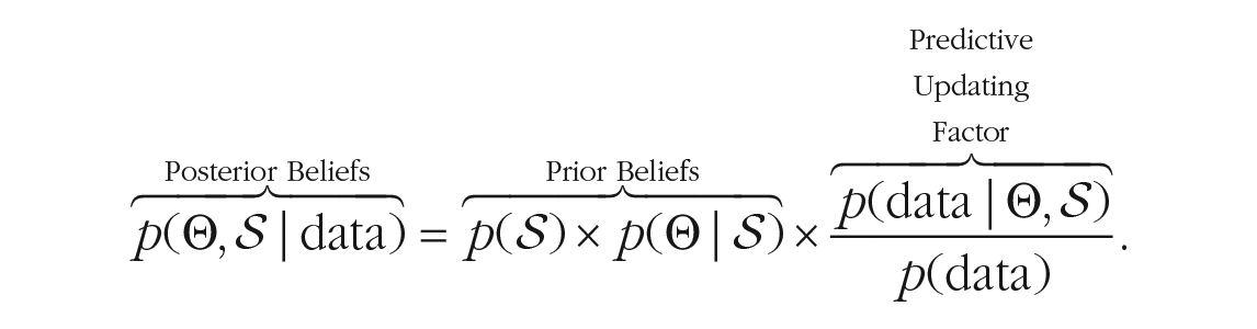
Specifically, prior beliefs about the structure and about the parameters are updated using a predictive updating factor, which evaluates how well the prior structures and the prior parameters have predicted the observed data. Structures and parameter values that predicted the observed data well increase in plausibility, whereas those with poor predictions suffer a decline (Wagenmakers et al., 2016). The Bayesian updating cycle is completed by using the posterior distribution as a prior distribution in future analyses.

This framework also allows one to use the data to test hypotheses about networks. For example, one may compare the predictive performance of two competing structures, say Structure 1 ( ${\mathcal{S}}_1$ ) and Structure 2 ( ${\mathcal{S}}_2$ ). Here, one can assess which of the two structures better predicted the observed data. This comparison is called the “Bayes factor” (Jeffreys, 1961; Kass & Raftery, 1995), and it equals the change from prior to posterior odds brought about by the data:

$$\stackrel{\mathrm{Posterior}\mathrm{Odds}}{\overbrace{\frac{p\left({\mathcal{S}}_1\mathrm{|data}\right)}{p\left({\mathcal{S}}_2\mathrm{|data}\right)}}}=\stackrel{\mathrm{Prior}\mathrm{Odds}}{\overbrace{\frac{p\left({\mathcal{S}}_1\right)}{p\left({\mathcal{S}}_2\right)}}}\times \stackrel{{\mathrm{Bayes}\mathrm{Factor}\mathrm{BF}}_{12}}{\overbrace{\frac{p\left(\mathrm{data|}{\mathcal{S}}_1\right)}{p\left(\mathrm{data|}{\mathcal{S}}_2\right)}}}.$$

(1)

The Bayes factor is a continuous measure of support. A Bayes factor ${\mathrm{BF}}_{12}=10$ indicates that the data are 10 times more likely under structure ${\mathcal{S}}_1$ than under structure ${\mathcal{S}}_2$ . Conversely, one can obtain the evidence of structure 2 over structure 1 with ${\mathrm{BF}}_{21}=\raisebox{1ex}{$1$}\!\left/ \!\raisebox{-1ex}{${\mathrm{BF}}_{12}$}\right.$ ; thus, ${\mathrm{BF}}_{12}=\raisebox{1ex}{$1$}\!\left/ \!\raisebox{-1ex}{$10$}\right.$ amounts to ${\mathrm{BF}}_{21}=10$ . If the Bayes factor ${\mathrm{BF}}_{12}$ equals 1, the data are equally likely under both structures. In practice, the convention is to consider Bayes factors between 3 and $\raisebox{1ex}{$1$}\!\left/ \!\raisebox{-1ex}{$3$}\right.$ as weak support for either structure and Bayes factors larger than $10$ or smaller than $\raisebox{1ex}{$1$}\!\left/ \!\raisebox{-1ex}{$10$}\right.$ as strong support (e.g., Jeffreys, 1961, Appendix B).

Facilitating Bayesian Analysis for Uncertainty Quantification in Networks

As outlined in the introduction, there are three types of uncertainties that researchers should acknowledge when analyzing networks: (1) structure uncertainty, (2) evidence for edge inclusion and exclusion, and (3) parameter precision. Below, we explain how Bayesian methods can quantify these uncertainties.

Goal 1: quantify structure uncertainty

Many network structures are possible (e.g., Fig. 1), and researchers must be able to assess the relative plausibility of the structures to report their network results with confidence. In the Bayesian approach to network analysis, a posterior structure probability expresses how likely a particular structure is given the data and can be used to compare the plausibility of different structures (see the Bayes factor in Equation 1). To obtain this posterior probability, a prior distribution on the structures must first be specified. ⁵ There are several ways to do this (e.g., Consonni et al., 2018).

In the simplest version, researchers specify only the prior probability of including edges (Mohammadi & Wit, 2019), which can fall between 0 and 1. More densely connected structures can be expected if higher edge-inclusion probabilities are specified and vice versa. Uniform or hierarchical priors on the structures could also be stipulated (Marsman et al., 2022). The uniform prior assumes that all $2^k$ structures are equally plausible a priori. ⁶ In the example in Figure 1, each structure would obtain one eighth of the prior probability. Hereby, the uniform prior ignores the complexity (i.e., the number of present edges) of the different network structures. In Figure 1, Structure 2 with one edge is as plausible as Structure 1 with no edges even though there are three different structures with one edge (i.e., Structures 2–4) and only one with no edges (i.e., Structure 1). In contrast to the uniform prior, the hierarchical prior takes the structure’s complexity into account. It assigns equal prior plausibility to each complexity and assumes that given a certain complexity, structures are equally plausible (Scott & Berger, 2006). In the exemplary Figure 1, the hierarchical prior assigns the prior mass equally across all four complexities; they are all assigned a prior plausibility of one fourth. Afterward, the prior mass in each complexity is equally spread across all possible structures. For example, Structure 4 is one structure among three that have a one-edge structure complexity (i.e., Structures 2–4). Therefore, Structure 4 is assigned a third of the prior probability of the one-edge structure complexity, thus, $\raisebox{1ex}{$1$}\!\left/ \!\raisebox{-1ex}{$4$}\right.\times \raisebox{1ex}{$1$}\!\left/ \!\raisebox{-1ex}{$3$}\right.=\raisebox{1ex}{$1$}\!\left/ \!\raisebox{-1ex}{$12$}\right.$ . In contrast, Structure 1 is the only structure with no edges present, therefore, its prior plausibility is $\raisebox{1ex}{$1$}\!\left/ \!\raisebox{-1ex}{$4$}\right.\times \raisebox{1ex}{$1$}\!\left/ \!\raisebox{-1ex}{$1$}\right.=\raisebox{1ex}{$1$}\!\left/ \!\raisebox{-1ex}{$4$}\right.$ . A potential drawback of the hierarchical prior is that Structure 8 as the most complex structure gets a relatively high probability, violating the principle of parsimony.

The prior probability of the structure is updated with the data to form the posterior probability. Computing this posterior probability analytically is challenging. Therefore, most Bayesian approaches use simulation-based techniques that update the structure in each iteration, including or excluding edges from the current structure to form a new structure. The proportion of times a particular structure is visited in the simulation is an unbiased estimate of the posterior structure probability (George & McCulloch, 1993). Equipped with the posterior structure probability, researchers can assess the uncertainty of the underlying structure and the network complexity. If the sampler visit many different structures, researchers must be careful because this indicates that there is uncertainty about the underlying structure.

Summary: quantify structure uncertainty
	Problem
	How certain can one be about a particular structure?
	How to
	Specifying a prior distribution on the network structures to obtain posterior probabilities for each structure. One can either specify a prior edge-inclusion probability or a uniform/hierarchical prior.
	Interpretation
	Observing only a handful of structures that cover a high amount of posterior probability indicates a high certainty about the network structure. Observing many structures, each covering only a small fraction of posterior probability, indicates high uncertainty about the network structure; interpret the network with caution.

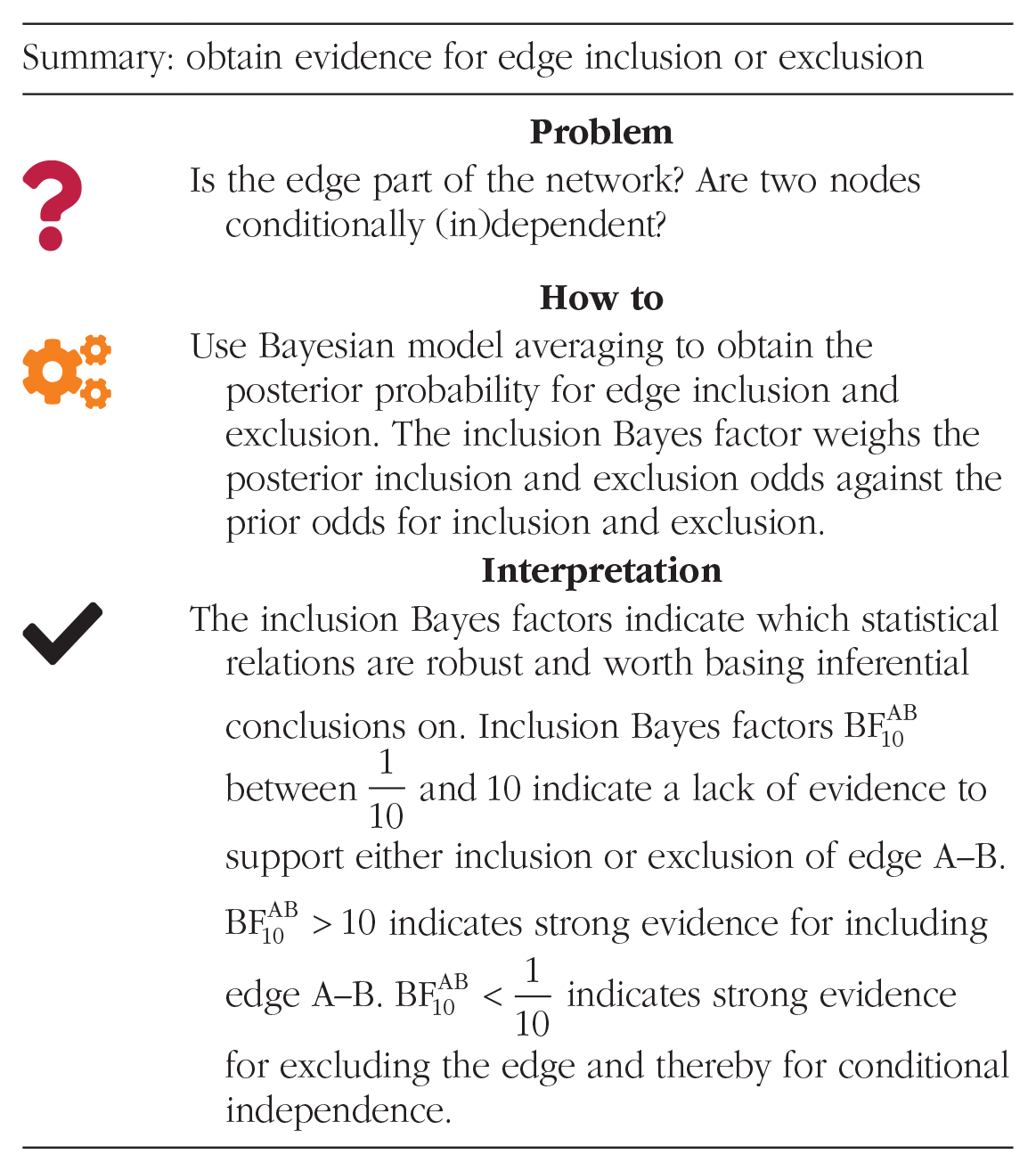
Goal 2: obtain evidence for edge inclusion or exclusion

A central goal of network analysis is to determine conditional (in)dependence, that is, the presence or absence of particular edges (Borsboom et al., 2021; Ryan et al., 2022). Although frequentist inference allows one to classify edge presence, it entails no information about edge absence. An estimated edge can be absent because either the edge weight has low precision/large standard errors (i.e., absence of evidence) or because it genuinely does not exist (i.e., evidence of absence; Keysers et al., 2020). Bayesians distinguish between absence of evidence and evidence of absence using the Bayes factor (or the posterior odds) in Equation 1. One can use the Bayes factor to compare how much more likely the data are under a structure in which the edge is present against a structure in which it is absent. This practice has been adopted to network models in which one compares the full model with all edges present against the full model with the focal edge removed (Williams & Mulder, 2020a). For example, one could compare Structures 1 and 2 in Figure 1 to obtain an evidence estimate for the edge A–B; this comparison assumes that all other edges are absent. Note, however, that one could have also compared Structures 7 and 8 and assumed all other edges are present. However, this comparison might yield a different evidence assessment because it is conditioned on a different set of edges. To obtain a single assessment of the posterior evidence for edge inclusion or exclusion, one may consider all possible structures simultaneously. This procedure is known as “Bayesian model averaging” (BMA; Hinne et al., 2020; Hoeting et al., 1999). Through BMA, one can obtain the prior and posterior odds of edge inclusion and exclusion and thereby obtain a Bayes factor for edge inclusion and exclusion:

$${\mathrm{BF}}_{10}^{\mathrm{AB}}=\stackrel{\mathrm{Posterior}\mathrm{Odds}}{\overbrace{\frac{p(\mathrm{edge}\mathrm{A}-\mathrm{B}\mathrm{included}|\mathrm{data})}{p(\mathrm{edge}\mathrm{A}-\mathrm{B}\mathrm{excluded}|\mathrm{data})}}}/\stackrel{\mathrm{Prior}\mathrm{Odds}}{\overbrace{\frac{p(\mathrm{edge}\mathrm{A}-\mathrm{B}\mathrm{included})}{p(\mathrm{edge}\mathrm{A}-\mathrm{B}\mathrm{excluded})}}}.$$

(2)

This inclusion Bayes factor is an aggregate of the previously described structure uncertainty. For networks, an edge-evidence plot illustrates the evidence for inclusion and exclusion for each edge (Huth et al., 2021), also illustrated in Figure 4a and 4b. In the network, edges are colored according to their inclusion Bayes factor: Red edges indicate evidence of absence, gray edges indicate the absence of evidence, and blue edges indicate evidence of presence. Equipped with the edge-evidence plot, researchers are able to decide which statistical relations are worth basing inferential conclusions on (i.e., red and blue edges) and which absent edges actually indicate conditional independence between variables (i.e., red edges). Gray edges indicate inconclusive evidence, and inferential conclusions should be avoided.

Summary: obtain evidence for edge inclusion or exclusion
	Problem
	Is the edge part of the network? Are two nodes conditionally (in)dependent?
	How to
	Use Bayesian model averaging to obtain the posterior probability for edge inclusion and exclusion. The inclusion Bayes factor weighs the posterior inclusion and exclusion odds against the prior odds for inclusion and exclusion.
	Interpretation
	The inclusion Bayes factors indicate which statistical relations are robust and worth basing inferential conclusions on. Inclusion Bayes factors ${\mathrm{BF}}_{10}^{\mathrm{AB}}$ between $\raisebox{1ex}{$1$}\!\left/ \!\raisebox{-1ex}{$10$}\right.$ and $10$ indicate a lack of evidence to support either inclusion or exclusion of edge A–B. ${\mathrm{BF}}_{10}^{\mathrm{AB}}>10$ indicates strong evidence for including edge A–B. ${\mathrm{BF}}_{10}^{\mathrm{AB}}<\raisebox{1ex}{$1$}\!\left/ \!\raisebox{-1ex}{$10$}\right.$ indicates strong evidence for excluding the edge and thereby for conditional independence.

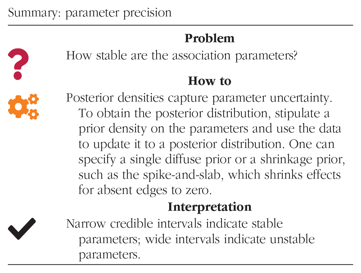
Goal 3: determine parameter precision

Assessing the uncertainty of association parameters between variables of a network is another crucial component of network analysis. In the Bayesian context, the posterior distribution of the parameters captures their stability. It expresses knowledge about the parameter after seeing the data. To obtain the posterior density, one must first stipulate a prior distribution on the parameters $p(\Theta |\mathcal{S})$ . A default choice is to specify an uninformative, diffuse prior distribution centered around zero. Note that this prior does not allow Bayes factors to be obtained. More advanced methods implement shrinkage priors such as the discrete or continuous spike-and-slab prior (e.g., Tadesse & Vannucci, 2022). The continuous spike-and-slab prior stipulates a prior density that is concentrated around zero for absent edges and a vague, zero-centered prior for present edges (for an illustration, see Fig. 2). Thus, the prior effectively shrinks an absent edge to a value close to zero (e.g., Marsman et al., 2022; Mohammadi, 2019). Present edges receive a zero-centered prior distribution with hardly any shrinkage; thus, the prior does not heavily influence the parameter estimate. Researchers can use these methods to obtain the parameter precision for a single structure (e.g., the most probable structure) or use BMA to obtain the parameter precision after averaging over all structures. The BMA estimate is preferred if there is uncertainty about the network’s structure because it considers both the uncertainty with respect to the structure and the parameter.

Fig. 2.

Illustration of the continuous spike-and-slab prior. Bayesian updating under the spike prior: the prior heavily shrinks the parameter estimate toward zero. Bayesian updating under the slab prior: the weakly informative prior hardly affects the posterior distribution.

One can summarize the posterior parameter distribution in several ways. Credible intervals are suitable measures for parameter uncertainty: Wide intervals indicate high uncertainty, and narrow intervals indicate reduced uncertainty. We propose to use the 95% highest posterior density interval because it is the shortest interval that captures 95% of the posterior distribution.

Summary: parameter precision
	Problem
	How stable are the association parameters?
	How to
	Posterior densities capture parameter uncertainty. To obtain the posterior distribution, stipulate a prior density on the parameters and use the data to update it to a posterior distribution. One can specify a single diffuse prior or a shrinkage prior, such as the spike-and-slab, which shrinks effects for absent edges to zero.
	Interpretation
	Narrow credible intervals indicate stable parameters; wide intervals indicate unstable parameters.

Software Implementations in R

In this section, we review available R (R Core Team, 2020) packages for the Bayesian analysis of networks and introduce a new user-friendly package, easybgm. The existing R packages allow estimating the most popular types of cross-sectional networks—that is, the Gaussian graphical model (GGM), Ising model, ordinal Markov random fields, and mixed-graphical model. First, we introduce the three major existing packages (i.e., BDgraph, BGGM, and bgms) below. Their performances are compared in the appendix. Second, we introduce the new package easybgm, which is a wrapper around the existing packages. Table 1 provides an overview of the functionalities of the packages. An annotated analysis script with example code for each package is available on OSF. ⁷

Table 1.

Overview of Software Packages for Cross-Sectional Bayesian Analysis of Networks

Package	Models	Function	Description	Input type	Prior specification	Features
BDgraph	Gaussian, mixed	bdgraph(data, type = c(“ggm”, “gcgm”))	Structure-selection algorithm in graphical models	Raw data or covariance matrix	g.prior: prior inclusion probability for edges (default = 0.5; range = 0–1); g.start: graph at start; df.prior: degrees of freedom for G-Wishart distribution, prior on the precision matrix (default = 3)	Provides model-averaged estimates of the precision matrix; missing values deleted listwise
	Gaussian, ordinal, Ising	bdgraph.mpl(data, method = c(“ggm”, “dgm”, “dgm-binary”))	Pseudolikelihood approximation of graphical models		alpha: hyperparameter of Dirichlet distribution; g.prior: prior inclusion probability for edges
BGGM	Gaussian, mixed, Ising	estimate(Y, type = (“continuous”, “mixed”, “binary”))	Algorithm for Bayesian inference in Gaussian (copula) graphical models	Raw data	prior_sd (default = .5): prior standard deviation of the matrix-F distribution	Provides parameter estimates and posterior edge-inclusion probabilities; imputes missing data
bgms	Ordinal, Ising	bgm(x)	Bayesian structure selection for ordinal Markov random field models	Raw data	interaction_prior: type of interaction prior distribution (default = unit information); threshold_alpha & threshold_beta: shape parameters of the Beta-prime prior for the thresholds (default = 1)	Provides posterior samples of the estimates and the underlying structures; missing values deleted listwise
easybgm	All	easybgm(data, type = (“continuous”, “binary”, “ordinal”, “mixed”)	User-friendly Bayesian estimation and visualization of networks	Raw data	Respective prior specification of the underlying packages	Provides a user-friendly wrapper for the Bayesian estimation of networks and an extensive suite of functions to visualize results

The R package BDgraph (Mohammadi & Wit, 2019) offers tools for the Bayesian analysis of networks for (a mix of) continuous, ordinal, and binary variables. The package consists of several simulation-based procedures for exploring the structure space, which is implemented in C++ with parallel computing capabilities. BDgraph can estimate GGMs to analyze continuous data (Mohammadi et al., 2023; Mohammadi & Wit, 2015), and Gaussian copula graphical models (GCGMs) to analyze (a mix of) ordinal, binary, and continuous data (Mohammadi et al., 2017; Vinciotti et al., 2022). The package also allows the estimation of a discrete-graphical model (DGM) for ordinal and binary data using a marginal pseudolikelihood approach (Dobra & Mohammadi, 2018). Users can provide either the raw data or the covariance matrix (for GGM and GCGM) and choose between three distinct sampling algorithms; the reversible-jump Markov chain Monte Carlo (MCMC), continuous-time birth–death MCMC, or hill-climbing algorithm. The specification of priors depends on the type of model to be estimated. For the GGM and the GCGM, users can specify the edge-inclusion probability (i.e., g.prior), the initial configuration of edge inclusion (i.e., g.start), and the degrees of freedom for the prior on the precision estimate (i.e., df.prior), which is a G-Wishart distribution. The higher the degrees of freedom is, the more informative the prior is. Alternatively, users can make use of a regularization prior through the closely related package ssgraph (Mohammadi, 2019). The package implements a continuous spike-and-slab prior distribution for the precision matrix. For a DGM, BDgraph stipulates a Dirichlet distribution on the prior precision matrix for which users can specify an alpha hyperparameter. The package output consists of the model-averaged precision estimates (i.e., can be transformed into partial interactions), the posterior-inclusion probability, and the visited structures. It does not allow for missing data handling.

The R package BGGM offers tools for estimating and testing graphical models (Williams & Mulder, 2020b). The BGGM package can estimate a GGM to analyze continuous data and a GCGM to analyze (a mix of) binary, ordinal, and continuous data. ⁸ Users can specify the prior standard deviation (i.e., prior_sd) of the matrix-F distribution, a scale mixture of Wishart distributions, stipulated on the precision matrix. The package output consists of the posterior mode of the model parameters and the posterior edge-inclusion probabilities. Unlike BDgraph, BGGM does not explore the structure space and thus cannot provide model-averaged estimates. However, contrary to the other packages, BGGM can handle missing data by imputing missing values (Buuren & Groothuis-Oudshoorn, 2011) and provides a wide variety of other features, such as one-sided edge testing (i.e., testing for a positive interaction) and estimating and testing subgroup differences.

Marsman and Haslbeck (2023) recently developed the bgms package that focuses on the Bayesian analysis of binary and ordinal Markov random field models. The package uses Bayesian variable-selection methods to model the underlying network structure. The methods are organized around two general approaches for Bayesian variable selection: (a) expectation-maximization (EM) variable selection (Ročková & George, 2014) and (b) Gibbs variable selection (George & McCulloch, 1993). The EM variable selection function bgm.em uses the continuous spike-and-slab prior specification of Marsman et al. (2022) stipulated on the pairwise interactions and generalizes it to Markov random field models for (mixed) binary and ordinal variables. The Gibbs variable selection function bgm, on the other hand, uses a discrete spike-and-slab prior distribution for the pairwise interactions, which can set the interactions to exact zeroes. To account for the discontinuity at zero, the Metropolis approach of Gottardo and Raftery (2008) is embedded in a Gibbs sampler. Currently, the slab distribution is either a unit-information type prior (for details, see Marsman and Haslbeck, 2023) or a Cauchy distribution with a scale that can be set by the user. A Beta-prime distribution is used for the exponentiated category parameters, and a uniform prior is used for the edge-indicator variables (i.e., the prior probability that an edge is included is $.5$ ). As output, the package provides the posterior distribution of both the structure and the parameter estimates, thus allowing for model-averaged estimates. The package currently deletes missing data listwise.

The reviewed R packages are powerful tools for a Bayesian analysis of networks. However, they can be difficult to use for researchers with limited programming experience. Therefore, we introduce a new R package, easybgm, that provides a user-friendly and intuitive set of functions for estimating all types of models and visualizing their results. Our package builds functions around the introduced R packages (i.e., BDgraph, bgms, and BGGM) and a large set of functions to help visualize the results. To initiate estimation, researchers specify the data set and the data type (i.e., continuous, mixed, ordinal, or binary). Based on the data-type specification, easybgm estimates the network using the appropriate R package (i.e., BDgraph for continuous and mixed data and bgms for ordinal and binary data). Users can deviate from the default package choice by specifying their preferred R package. Based on the different estimates, easybgm outputs the results, including the parameter estimates, the posterior-inclusion probability, the inclusion Bayes factor, and optionally the posterior samples of the parameters and strength centrality samples. In addition, easybgm comes with an extensive set of visualization functions, such as the plots shown in the example of this article. In particular, users can obtain a network plot showing the parameter estimates, an edge-evidence plot showing the inclusion Bayes factor, and various plots to assess the structure uncertainty.

Example: Mental Health and Personality

In this section, we illustrate the Bayesian benefits through a concrete example. In particular, we explore whether and to what extent common personality traits are associated with mental-health concerns. We use an open data set on the Depression, Anxiety, and Stress scales (DASS) from the openpsychometric website, administered between 2017 and 2019. For this tutorial, we used a random subset of 2,000 out of 39,775 participants. We include 13 nodes in the network, representing scores of the three mental-health subscales (i.e., depression, anxiety, and stress) and 10 personality traits. We encourage readers to download the openly available data set “Answers to the Depression Anxiety Stress Scales” at https://openpsychometrics.org/_rawdata/ and explore the cross-sectional Bayesian analysis of networks with the annotated scripts. ⁹ Following previous research, we specified a uniform prior on the network structure (i.e., prior edge-inclusion probability of 0.5) and a $\mathrm{G}-\mathrm{Wishart}(d,D)$ prior on the precision matrix with 3 degrees of freedom d and an identity matrix for D (Hinne et al., 2020).

Structure uncertainty

There are $2^{78}$ possible network structures for this exemplary network, and a priori, we assigned equal probability to all of them. Results are shown in Figure 3. The MCMC algorithm visited $634$ distinct network structures. Figure 3a shows the posterior probability of the structures ordered according to their posterior probability. Although four structures show a slightly higher posterior probability than others, no single structure claims a significant fraction of the posterior probability. This means that we are highly uncertain about the underlying structure and should acknowledge that several structures are plausible for the data at hand. At the same time, most of the identified structures have a similar complexity in that they have a similar number of edges (see Fig. 3b). We assigned most prior mass to structures with $50\mathrm{\%}$ of all edges present (i.e., see that the gray xs peak at 39 edges). After observing the data, we conclude that all posterior probability concentrates on structures with 51 edges at a minimum and that more than 75% of the posterior probability concentrates on structures with 53 to 58 edges. In sum, although we are very uncertain about the underlying structure, we can be relatively sure about its complexity. In contrast, in the frequentist approach, one would merely obtain a single optimal structure without its associated uncertainty and obtain a single complexity estimate. One would base all inferential decisions on the most plausible structure, although there are several similarly plausible structures; the inferential decisions would have a high chance to be flawed.

Fig. 3.

The posterior probabilities of different network structures and their complexity. The left plot indicates the posterior probabilities of the visited structures, sorted from the most to the least probable. Each dot represents one structure. The gray dashed line denotes the prior probability for each structure. The right plot indicates the posterior probability for different structure complexities, where complexity comprises the network density. The gray xs denote the prior probability for each structure complexity.

Edge evidence

We illustrate the evidence for inclusion and exclusion for each edge with the networks in Figures 4a and 4b. The edge-evidence plot aids researchers in deciding which edges provide robust inferential conclusions: Red edges indicate evidence for edge absence, gray edges indicate the absence of evidence, and blue edges indicate evidence for edge presence. Figure 4a shows edges with an inclusion Bayes factor larger than 1, deemed included. Nodes mostly link within the respective clusters: The three mental-health measures are all connected, and most personality traits are conditionally dependent. Several links connect mental-health measures and personality factors. In addition, there are many edges that are included in the network but for which we do not have sufficient evidence for the inclusion (i.e., gray edges), especially for the edges linking to extraverted and disorganized. Figure 4b shows edges with an inclusion Bayes factor lower than 1 deemed excluded. Anxiety is conditionally independent of several personality items, and open is conditionally independent from mental-health and personality factors. Furthermore, several edges are deemed excluded, but there is not sufficient evidence to conclude edge absence (i.e., gray edges). Separating the evidence of absence (i.e., red edges) and absence of evidence (i.e., gray edges) is a unique benefit of the Bayesian approach and thus allows one to obtain evidence for conditional independence. In contrast, the frequentist approach would only be able to deem edges included, not whether there is evidence of edge absence.

Fig. 4.

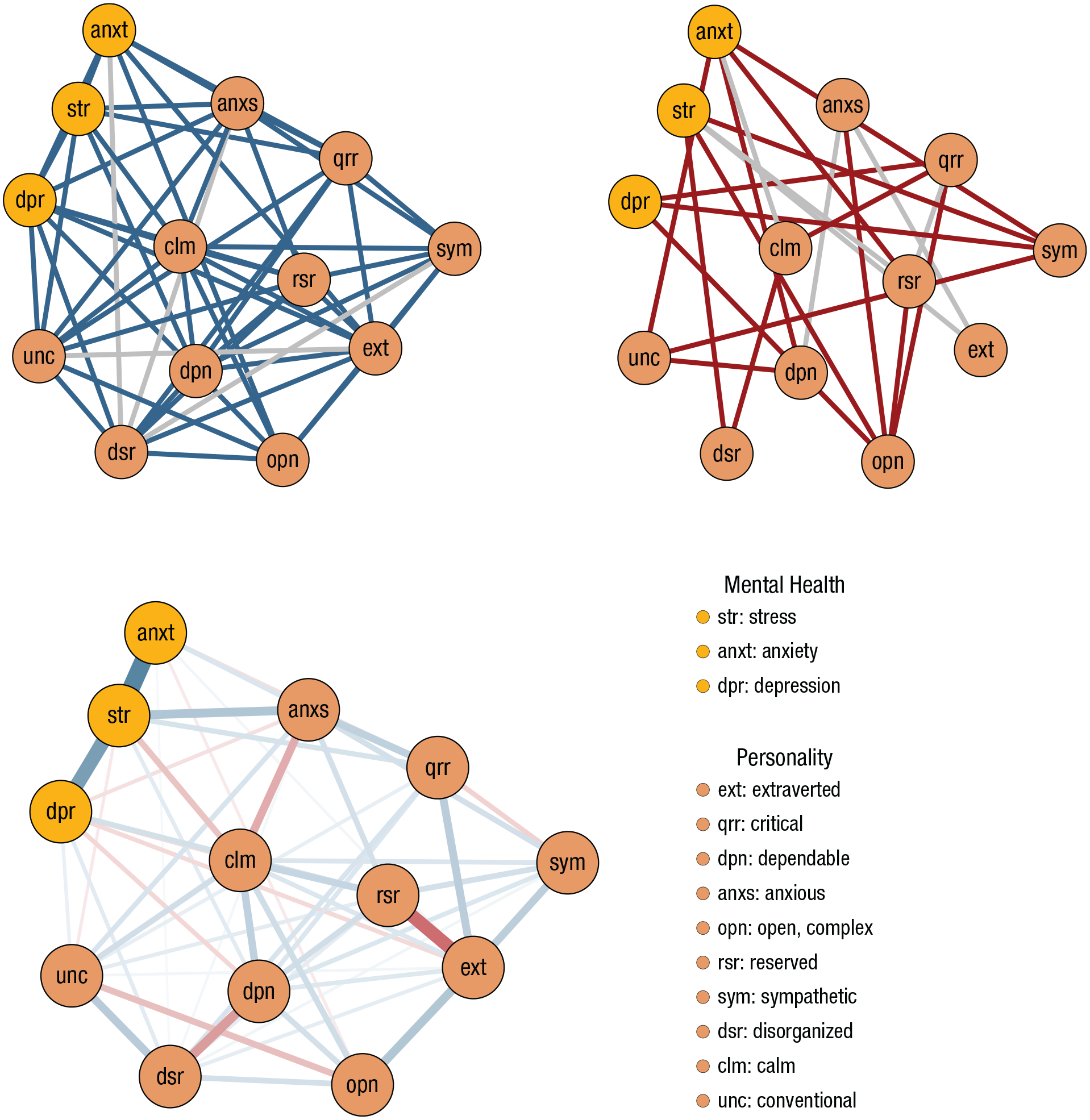
Networks showing the edge-evidence plots (top row) and the respective strength and nature of associations (bottom row). (a) Edge-evidence plot showing present edges (i.e., BF₁₀ > 1), where blue edges represent evidence for inclusion (BF₁₀ > 10) and gray edges absence of evidence (1 < BF₁₀ < 10). (b) Edge-evidence plot depicting absent edges (i.e., BF₁₀ < 1); evidence for exclusion is shown as red (BF₁₀ < 0.1), and inconclusive evidence is shown as gray (0.1 < BF₁₀ < 1). (c) The parameter-estimate plot shows all edges with an inclusion Bayes factor larger than 1. Edge thickness and saturation represent the strength of the association; the thicker the edge, the stronger the association. Red edges indicate negative relations, and blue edges indicate positive associations.

Parameter estimation and precision

In Figure 4c, we show the parameter-estimate plot of included edges, thus, edges with an inclusion Bayes factor of at least 1 (i.e., commonly called “median probability model”). Researchers could also choose other cutoffs of parameters to be shown (e.g., edges with strong evidence for inclusion; ${\mathrm{BF}}_{10}>10$ ). We advocate the median-probability model that has been shown to have optimal predictive properties (Barbieri et al., 2021). The three mental-health outcomes are all positively related; stress relates strongly to both depression and anxiety. Stress is furthermore positively connected to the personality-variable anxious and negatively connected to calm. Strong negative associations can be found between several personality items, for example, between extraverted and reserved and between open and unconventional.

As an illustration, Figure 5 shows the posterior distribution of two parameters of the network model obtained through BMA. Figure 5a shows a near-symmetrical distribution of an edge parameter in which most posterior mass lies between $0.1$ and $0.2$ . We can be confident that the parameter lies somewhere in this interval. Figure 5b paints a different picture: The distribution is bimodal such that some mass is distributed just above 0 and another large amount between $0.03$ and $0.1$ . The plot highlights the influence of BMA. This edge is absent in many plausible structures; in those, the parameter will be close to 0. However, the edge is present in many other plausible structures; here, the parameter lies between $0.03$ and $0.1$ . We are thus uncertain if the edge should be included and how strong the connection is. In contrast, in the frequentist approach, researchers would merely obtain the parameter estimate. To obtain a measure of uncertainty, one would obtain a bootstrapped confidence interval, which is negatively affected by the lasso regularization (e.g., see Bühlmann et al., 2014; Pötscher & Leeb, 2009).

Fig. 5.

Posterior distribution of two network parameters. Densities show the model-averaged estimate of both parameters. The left plot shows an estimate of an included edge and the right plot of an edge without enough evidence to conclude on inclusion or exclusion: (a) included edge, (b) inconclusive edge.

Advanced benefits

On the basis of the three Bayesian benefits, researchers can facilitate other benefits for their analysis, for example, obtaining credible intervals around centrality estimates. Researchers often use centrality measures to obtain aggregated information for each node, for example, the connectedness quantified in the strength centrality. Credible intervals for strength centrality can be obtained by calculating the centrality measure for each sample of the posterior parameter distribution. Strength-centrality estimates and highest density intervals (HDIs) are shown in Figure 6. The higher the centrality is, the more strongly connected the node is; error bars represent the 95% HDI. Stress is the most central node; the least central nodes were conventional and sympathetic. The HDIs of all variables are narrow, and thus, we can be relatively confident about the strength-centrality estimates.

Fig. 6.

Strength centrality. The yellow dots and lines represent the mental-health variables, and the orange dots and lines are the personality items.

JASP Implementation

BDgraph’s functionality (Mohammadi & Wit, 2019) was recently implemented in JASP (JASP Team, 2018), allowing researchers without programming experience to estimate networks in a Bayesian framework. ¹⁰ In this section, we walk the reader through performing a Bayesian analysis of networks in JASP using the previous example. Readers can find the associated annotated JASP script on OSF. ¹¹ We refer readers new to JASP to its tutorial (Wagenmakers et al., 2018). Figure 7 provides a screenshot of the Bayesian network module.

Fig. 7.

Screenshot of the Bayesian network implementation of BDgraph in JASP. The left panel shows the analysis input options, and the right panel shows the associated output.

Input

To initiate the estimation, researchers specify the variables to include in the network, after which they specify the estimation method; implemented are “ggm” (i.e., Gaussian graphical model for continuous data) or “gcgm” (i.e., Gaussian copula graphical model, for a mix of binary, ordinal, count and continuous data). Subsequently, JASP will output the number of present edges in the estimated network. Note that “gcgm” is computationally intensive and might take substantial time to show output.

Output

Users have several options to gain insight into the underlying network and its three uncertainties. First, to quantify the structure uncertainty, users can find the “Posterior Structure Probability” and the “Posterior Complexity Plot” options in the “Network structure selection” tab. Second, users can assess the support for individual edges via a table and a plot. By default, the table contains the posterior-inclusion probabilities for each edge in the network. With one click, the user can opt to show Bayes factors instead: for inclusion (i.e., ${\mathrm{BF}}_{10}$ ), exclusion (i.e., ${\mathrm{BF}}_{01}$ ), or the log-transformed inclusion Bayes factors (i.e., log( ${\mathrm{BF}}_{10}$ )). The edge-evidence plot offers a visual representation of these results in which users can specify which edges to show (e.g., only edges with evidence for inclusion). Third, users can gain insight into the model parameters and their precision. The weight table offers the posterior means of the model parameters obtained using BMA (Hinne et al., 2020; Porwal & Raftery, 2022). The network plot provides a visual representation of these estimates, showing edges with an inclusion Bayes factor larger than 1 $0.5$ .

Advanced specifications

Centrality measures

In the “Graphical options” tab, users can choose which measures the centrality plot should display. By default, it shows the most common centrality measures: strength, betweenness, closeness, and expected influence. The Bayesian network module provides posterior means and the option for 95% HDIs for the centrality measures.

Sampling options

BDgraph works with MCMC sampling. Users can specify the number of iterations for the MCMC-sampling procedure. Estimates become more precise if more iterations are used, but the wait is longer. By default, JASP runs the sampler for $10,000$ iterations. Discarding the first samples is common practice because the sampler is still converging. Users can specify the number of iterations to discard with the burn-in period. As a rule, the burn-in should not exceed half the total number of iterations.

Prior

The user can specify prior beliefs about the network’s structure $\mathcal{S}$ and parameters Θ. The edge-inclusion probability (i.e., g.prior) defines the prior on the structure. The higher the value is, the higher the assumed structure density is, where the default value is $0.5$ . In addition, the initial configuration edge inclusion (i.e., g.start) specifies the initial network for the MCMC sampling, which is either empty (i.e., no edges present; default) or full (i.e., all edges present). The prior distribution for the network parameters is a G-Wishart distribution. Users can specify the degrees of freedom for this distribution (i.e., df.prior); the default is set to 3. The higher the degrees of freedom are, the more informative the prior is. For users unfamiliar with the Bayesian analysis of networks, we recommend starting with the default prior options in JASP.

Challenges and Outlook

Notwithstanding the benefits outlined above, the Bayesian approach comes with challenges of its own. First, Bayesian versions of some network-analysis tools are unavailable or concealed for a general audience because of advanced statistical writing. Therefore, Bayesian enthusiasts might fall back to frequentist alternatives. However, recent years have seen an insurgence of Bayesian tools for network analysis. For example, Bayesian tools for testing network differences in subgroups were formulated in the R package BGGM (Williams et al., 2020; Williams & Mulder, 2020b), and credible intervals for centrality estimates became available (Huth et al., 2021; Jongerling et al., 2023; Williams & Mulder, 2020a). Furthermore, through the outlined R package easybgm and the JASP implementation, researchers can analyze their data with limited or no prior programming experience.

Second, the Bayesian estimation of networks is computationally intensive, especially with the structure-selection step being cumbersome. The model space of $2^k$ possible structures (i.e., k being the number of parameters) is vast and explodes with increasing network size. The immensity of the model space also leads to uncertainty in estimating the posterior probability of network structures. There are simply too many structures over which one has to distribute the posterior probability, sometimes referred to as “dilution” (Clyde, 1999; George, 1999). Model averaging helps to form robust estimates, yet BMA does require running the sampling routines sufficiently long to produce these estimates.

Finally, the specification of appropriate prior distributions is not straightforward, yet their choice can influence the results. This concern holds for all Bayesian applications and is discussed in other work (see e.g., Wagenmakers et al., 2018). Robustness checks of priors are a tool to address this issue because they allow one to determine that conclusions do not rely solely on a particular prior specification. At the same time, informed priors could advance statistical inference by implementing prior knowledge or theory in the inferential cycle. This could be particularly promising in idiographic-network modeling (Burger et al., 2022) because such models are difficult to fully recover with the available data (Mansueto et al., 2022).

Concluding Comments

In this article, we provided a conceptual introduction to Bayesian analysis for psychometric, cross-sectional networks and demonstrated its application in assessing the interrelations of personality traits with mental health in a tutorial. The Bayesian approach provides the applied researcher with a tool for sound inferential conclusions, particularly through quantifying structure uncertainty, determining evidence for edge inclusion and exclusion, and quantifying parameter precision. With its conceptual introduction, newly developed R package easybgm, and user-friendly JASP implementation, we hope this work will enable a broader audience to make use of the Bayesian benefits to network psychometrics.