Sage Journals: Discover world-class research

Abstract

Analysis of variance (ANOVA) is widely used to assess the influence of one or more experimental (or quasi-experimental) manipulations on a continuous outcome. Traditionally, ANOVA is carried out in a frequentist manner using p values, but a Bayesian alternative has been proposed. Assuming that the proposed Bayesian ANOVA is closely modeled after its frequentist counterpart, one may be surprised to find that the two can yield very different conclusions when the design involves multiple repeated-measures factors. We illustrate such a discrepancy with a real data set from a two-factorial within-subject experiment. For this data set, the results of a frequentist and Bayesian ANOVA are in a disagreement about which main effect accounts for the variance in the data. The reason for this disagreement is that frequentist and the proposed Bayesian ANOVA use different model specifications. As currently implemented, the proposed Bayesian ANOVA assumes that there are no individual differences in the magnitude of effects. We suspect that this assumption is neither obvious to nor desired by most analysts because it is untenable in most applications. We argue here that the Bayesian ANOVA should be revised to allow for individual differences. As a default, we suggest the standard frequentist model specification but discuss a recently proposed alternative and provide guidance on how to choose the appropriate model specification. We end by discussing the implications of the revised model specification for previously published results of Bayesian ANOVAs.

Keywords

ANOVA repeated-measures ANOVA Bayesian inference random slopes JASP

Analysis of variance (ANOVA) is ubiquitous in experimental psychology, in which it is used to assess the influence of one or more experimental (or quasi-experimental) manipulations on a continuous outcome. For instance, in a Stroop task (Stroop, 1935) participants are asked to name the color of a printed word. It is typically found that participants respond faster when a word’s meaning and color are congruent (e.g., blue displayed in a blue font) and slower when these are incongruent (e.g., blue displayed in a red font). The relation between the congruency of the colored words and the response times of the participants can be analyzed with a (repeated-measures) ANOVA. Traditionally, ANOVAs are carried out in the frequentist paradigm, and p values are used to arrive at scientific conclusions. Rouder et al. (2012) proposed a general Bayesian modeling framework for linear models that they used to develop an influential Bayesian alternative approach to ANOVA (cited over 1,500 times; see also Rouder et al., 2017; van den Bergh et al., 2020). Assuming that this Bayesian ANOVA is closely modeled after its frequentist counterpart, one may be surprised to find that the two can yield very different conclusions when the design involves multiple repeated-measures factors. Using a real data set, we show that discrepancies between frequentist and the proposed Bayesian ANOVA reflect the fact that they use different model specifications. We believe that many analysts are unaware of this difference and, critically, that the model specification in the Bayesian ANOVA is usually inappropriate.

The frequentist and Bayesian approaches differ in how they model individual differences. The frequentist ANOVA allows for individual differences in treatment effects. The model specification includes separate error strata (i.e., Participant × Treatment interaction or random slopes) for all but the highest order repeated-measures interaction. The proposed Bayesian ANOVA does not. It includes random intercepts only (RIO)—we henceforth refer to this as the RIO-model specification. Although their modeling framework allows for random slopes, Rouder, Morey, and colleagues recommended to omit them (Rouder et al., 2012, 2017). This recommendation was based on two concerns: Random-slope terms greatly increase model complexity and complicate the interpretation of fixed effects—if a substantial portion of participants has a negative effect, does it make sense to interpret a positive fixed effect? These are important concerns, but we believe the omission of random slopes is inappropriate in most applications: The RIO-model specification implies the strong assumption of the complete absence of individual differences in the magnitude of the effects—a universal effect size for every subject. We are hard-pressed to think of any psychological effects for which this assumption seems plausible. We therefore recommend including random slopes in Bayesian ANOVA models.

Like the frequentist ANOVA, our recommended model specification contains the maximal set of random effects (MRE), which is why we henceforth refer to it as the MRE-model specification. Pivoting to the MRE-model specification is also consistent with recommendations within the broader framework of mixed models (Barr et al., 2013; Oberauer, 2022; van Doorn et al., 2023), of which repeated-measures ANOVA is a special case. For example, Oberauer (2022) showed in a simulation study on mixed models that, in the presence of random slopes, the use of RIO models can inflate Bayes factors and increases the risk of false-positive conclusions; we use a real data example to show that RIO models can similarly cause such questionable results in repeated-measures ANOVA. In addition to relaxing an untenable assumption, a universal effect size for every subject, the Bayesian MRE ANOVA resolves nontrivial differences in conclusions between the frequentist and Bayesian approach, such as the one we demonstrate below. The Bayesian MRE ANOVA relies on the modeling framework by Rouder et al. (2012) and may be thought of as a revision of the Bayesian RIO ANOVA as recommended in previous work (Rouder et al., 2012, 2017) and implemented in popular software, for example, the function anovaBF() from the R package BayesFactor (Morey & Rouder, 2021), which the statistics program JASP inherits.

The outline of this article is as follows. First we introduce a real data set that we use to illustrate the divergence between the frequentist and Bayesian results using JASP (JASP Team, 2022). We then explain the different model specifications and demonstrate that the discrepancy is resolved with a Bayesian MRE ANOVA, which is implemented in JASP Version 0.16.3. Afterward we discuss the merits and demerits of both model specifications, as well as a third model specification that was recently proposed (Rouder et al., 2023). The article concludes with a discussion on how RIO ANOVA has affected published results of Bayesian ANOVAs.

Example Data: Stroop Effect

To illustrate how the model specification leads to discrepancies between frequentist and Bayesian ANOVA, we use an empirical data set kindly provided by Ronen Hershman and publicly available in the JASP Data Library (Hershman et al., 2022; Wagenmakers et al., 2020). The data were collected in an experiment on the Stroop effect (Stroop, 1935). Participants read color words (here blue, green, yellow, or red), which were presented in one of four font colors (blue, green, yellow, or red). The combination of color word and font color could be either congruent (e.g., blue displayed in a blue font) or incongruent (e.g., blue displayed in a red font). Participants were asked to ignore the meaning of the word and press one of four response buttons to indicate the font color. This paradigm is well known to produce the Stroop effect: Participants respond faster (and more accurately) to congruent than incongruent word-font color combinations; that is, participants appear to be unable to ignore the meaning of the words. In addition to congruent and incongruent combinations, the study at hand used neutral combinations of words and font color (e.g., the letters XXXX displayed in red font) to separately estimate the extent to which congruent combinations facilitate performance and incongruent combinations harm performance. The goal of the study was to investigate how the Stroop effect is affected by breaks from the task; consequently, the sequence of Stroop trials was interspersed with “break” trials (i.e., trials in which a black square, the rest stimulus, signaled that no response was required). This design makes it possible to compare performance on trials preceded by another Stroop trial with that on trials preceded by a break trial. Hence, the experiment used a 3 (Congruency: congruent vs. neutral vs. incongruent) × 2 (Preceding Trial, or PT: break vs. Stroop task) repeated-measures design. Each participant completed 144 congruent, neutral, and incongruent Stroop trials (totaling 432 trials) as well as 432 break trials in random order. Trials with incorrect or missing responses were excluded, and participants with less than 40 valid trials per condition were excluded from the analysis.¹ The raw data of all 19 participants are displayed in Figure 1. The top left of Figure 1 shows the average response times of the break and Stroop trials in each congruency condition, and the bottom left shows the associated within-subject differences; their average appears to be close to zero, suggesting that the nature of the PT has little systematic impact on Stroop performance. The top right of Figure 1 shows the average response times of congruent, neutral, and incongruent trials in each PT condition, and the bottom right shows the associated differences; it seems that, on average, congruent responses are faster than incongruent responses, congruent and neutral responses are approximately equally fast, and incongruent responses are slower than neutral responses.

Fig. 1.

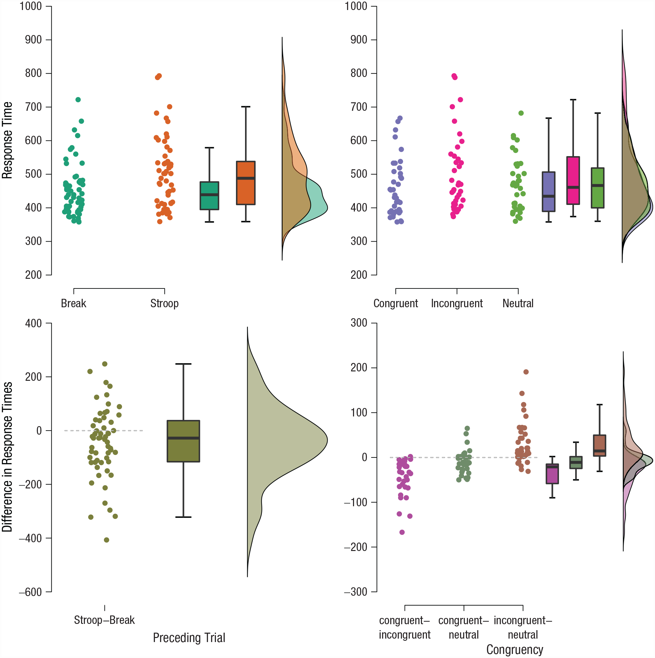
Raincloud plots of the raw data from the Hershman Stroop Study. The average response times (y-axis) are shown for the break and Stroop conditions (x-axis) in each congruency condition (top left). The average response times for the congruent, neutral, and incongruent conditions (x-axis) are shown for the preceding trial condition (top right). Pairwise differences in response time (y-axis) are shown between the break and Stroop conditions (bottom left). Pairwise differences in response time (y-axis) are shown for all pairs of the congruency factor (bottom right). Box plots and density estimates are shown on the right of each panel. See text for details.

Discrepancy between frequentist and Bayesian ANOVA

The frequentist repeated-measures ANOVA indicates that the main effect of PT and the interaction between PT and congruency are not significant, $F (1, 18) = 2.24$ , $p = . 152$ , and $F (2, 36) = 2.30$ , $p = . 115$ , whereas the main effect of congruency is significant, $F (2, 36) = 22.16$ , $p < . 001$ (Table 2).² Although Mauchly’s sphericity test is significant and thus the assumption of sphericity is violated, the Greenhouse-Geisser and Huyhn-Feldt corrections yield the same qualitative pattern as the uncorrected results (see Table A1).

In the Bayesian ANOVA, we use the Bayes factor to compare all models to the model that best predicts the data (in this case the model including only the PT effect). The results are shown in Table 1, which lists models according to their performance in decreasing order, with the best model in the first row and the worst model in the last row. The first column displays the predictors in the model. The second column and third column, P(M) and P(M|data), respectively, show the prior and posterior model probabilities. The fourth column, ${BF}_{10}$ , shows the Bayes factor relative to the best performing model. The final column, error, contains the relative error associated with the numerical method used to approximate the Bayes factors.

Table 1.

Bayesian Comparisons of Models Including Random Intercepts but Not Random Slopes for Participants

Models	P(M)	P(M\|data)	BF₁₀	Error
PT	0.200	0.444	1.000
PT + congruency	0.200	0.430	0.969	0.430
PT + congruency + PT × Congruency	0.200	0.073	0.165	0.503
Null model (including subject)	0.200	0.030	0.067	0.344
Congruency	0.200	0.023	0.052	0.366

Note: Model formulas omit random intercepts for participants (i.e., + participant), which are included in all models. P(M) and P(M|data) indicate prior and posterior model probabilities, respectively; ${BF}_{10}$ indicates Bayes factors relative to the best performing model; and error is the relative error associated with the numerical method used to estimate the Bayes factors. PT = preceding trial.

Most importantly, the worst performing model includes only congruency as a predictor—the only predictor associated with a significant p value. Note, however, that these Bayes factors are not directly analogous to any of the standard F-tests in the frequentist ANOVA. Rather than comparing each model to the best model of the set, frequentist F-tests reflect model comparisons designed to assess the unique variance associated with each factor. To contrast the frequentist and Bayesian results more directly, we first calculate Bayes factors that reflect the same model comparisons as the F-tests.³ The results are shown in Table 2 in the column ${BF}_{10}$ for the Bayesian RIO analysis. For the effect of congruency, the analogous Bayes factor quantifies the evidence for the model with PT + congruency relative to the model with only PT: ${BF}_{10} = 0.969 / 1.000 = 0.969$ . The data just barely favor the model without congruency. Likewise, for the effect of PT we compare the model with PT + congruency to the model with only congruency: ${BF}_{10} = 0.969 / 0.052 \approx 18.482$ . The data provide strong evidence for an effect of PT. In other words, executing the same model comparisons as the F-tests has not resolved the striking discrepancy between the Bayesian and the frequentist analyses.

Table 2.

Comparison of ANOVA Results for the Hershman Stroop Study Across Different Analytic Approaches

Frequentist						Bayesian
				Random intercept only		Maximal set of random effects		Simultaneous fixed and random effects
Factor	df	F	p	${BF}_{10}$	${BF}_{Inclusion}$	${BF}_{10}$	${BF}_{Inclusion}$	${BF}_{10}$	${BF}_{Inclusion}$
PT	1, 18	2.242	.152	18.482	11.885	0.781	0.983	8.556 · 10²⁸	2.729 · 10¹⁴
Congruency^a	2, 36	22.158	< .001	0.969	0.741	7,074.832	6,757.451	2.75 · 10⁴	2.982 · 10⁴
PT × Congruency^a	2, 36	2.297	.115	0.170	0.316	0.890	1.560	0.627	2.506

Note: Column spanners indicate the random-effects structure assumed in the Bayesian ANOVA models; the maximal set of random effects is the new default in JASP. ANOVA = analysis of variance; PT = preceding trial; ${BF}_{10}$ = Bayes factor model comparison; ${BF}_{Inclusion}$ = model-averaged Bayes factor of model including an effect relative to model excluding it.

Mauchly’s test of sphericity indicates that the assumption of sphericity is violated (p <. 05).

However, the Bayesian analysis is based on a comparison between two specific models. This approach ignores the possibility that both models may be outperformed by one or more of the other candidate models. The uncertainty about which models are the most appropriate can be taken into account by averaging across all models (Hinne et al., 2020; Hoeting et al., 1999). For example, to assess the support for the effect of PT, the performance of all models that include PT (i.e., PT, PT + congruency, and PT × Congruency) is contrasted to the performance of all models that exclude PT (i.e., congruency) and the null model. The resulting inclusion Bayes factor takes the entire model space into account. Applying the inclusion Bayes factor approach yields the results shown in the ${BF}_{Inclusion}$ column in Table 2 for the Bayesian RIO analysis. As the table shows, the model-averaged inclusion Bayes factor ( ${BF}_{Inclusion}$ ) yields results that are similar to the simple model comparisons ( ${BF}_{10}$ ): Averaging across all models there is strong evidence in favor of including PT and weak evidence against congruency and PT × Congruency.

In sum, regardless of the specific Bayes factor approach that is taken (i.e., comparing against the best model, contrasting two specific models, model averaging), the results indicate little evidence regarding the significant effect of congruency but strong evidence for the nonsignificant effect of PT. This conclusion, however, appears to contradict the data pattern in Figure 1 (bottom left), which suggests that there is no effect of PT.

Different model specifications

The notable discrepancies between the frequentist and Bayesian results outlined in the previous section are caused by a difference in the underlying model specification. The frequentist ANOVA uses the MRE-model specification, which specifies all estimable Participant × Treatment interactions (i.e., error strata) for repeated-measures variables (see Appendix of Barr et al., 2013). In mixed-model terms, these Participant × Treatment interactions amount to random slopes—they allow for individual differences in the effects of PTs and congruency. For our example, the full model including all factors is RT ~ 1 + congruency × PT + (1 + congruency + PT | participant).⁴

In contrast, the Bayesian RIO ANOVA omits the Participant × Treatment interactions; only the participant main effect (i.e., the random intercept) is included. For our example, the full model including all factors is RT ~ 1 + congruency × PT + (1 | participant). This RIO-model specification implements the unreasonable assumption that there are no individual differences in the magnitude of the effects. Assuming interindividually constant main effects is unique to the current default Bayesian ANOVA and causes the divergence from the frequentist ANOVA. Moreover, this assumption is likely not obvious to most analysts and at odds with what they expect when conducting repeated-measures ANOVA.

RIO ANOVA is clearly misspecified for our example data: There is substantial variability in participants’ PT effects, as summarized in Table 3—the random-slope variance for PT even exceeds the random-intercept variance. When we repeat the Bayesian ANOVA with the standard model specification by including random slopes (Table 4), the conclusions change substantially: The model including only congruency is the best model, whereas the model including only PT is the worst model—a conclusion opposite to the one from our previous Bayesian RIO ANOVA. The results from simple model comparisons and model averaging are now both in agreement with the frequentist repeated-measures ANOVA. Table 2 summarizes the results for the frequentist ANOVA, the Bayesian RIO ANOVA without random slopes, and the Bayesian MRE ANOVA with random slopes.

Table 3.

Estimates of Participant Random-Effect Variances and Standard Deviations from a Maximal Hierarchical Linear Model for the Aggregated Data

Group	Effect	Variance	SD
Participants	Intercept	3767.15	61.38
	Congruency	228.73	15.12
	PT	4186.87	64.71
Residual		536.82	23.17

Note: PT = preceding trial.

Table 4.

Bayesian Comparisons of Models Including Random Intercepts and Random Slopes for Participants

	P(M)	P(M\|data)	BF₁₀	Error
Congruency	0.200	0.404	1.000
PT + congruency	0.200	0.315	0.781	3.953
PT + congruency + PT × Congruency	0.200	0.281	0.695	6.076
Null model (including subject and random slopes)	0.200	5.408 · 10⁻⁵	1.339 · 10⁻⁴	0.220
PT	0.200	4.457 · 10⁻⁵	1.103 · 10⁻⁴	6.891

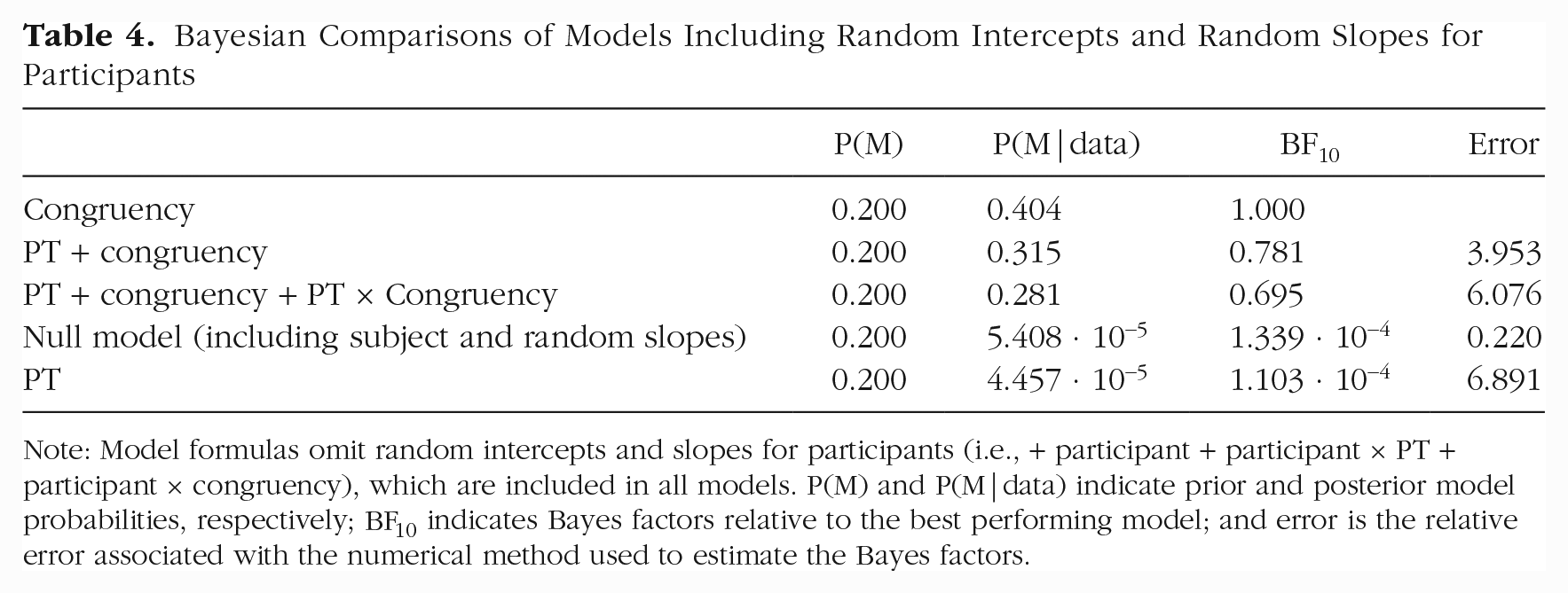
Note: Model formulas omit random intercepts and slopes for participants (i.e., + participant + participant × PT + participant × congruency), which are included in all models. P(M) and P(M|data) indicate prior and posterior model probabilities, respectively; ${BF}_{10}$ indicates Bayes factors relative to the best performing model; and error is the relative error associated with the numerical method used to estimate the Bayes factors.

A third model specification that sits between RIO and MRE ANOVA was recently proposed (Rouder et al., 2023). Whereas RIO ANOVA always omits random slopes, MRE ANOVA never omits them—even if the corresponding fixed effect is removed from the model. For example, the model that includes a main effect of PT but not congruency is RT ~ 1 + PT + (1 + congruency + PT | participant). Rouder et al. (2023) argued that this implies the unreasonable assumption that, when an effect is absent, the population is split between individuals with positive and individuals with negative effects, which cancel out to a null effect overall. Instead, Rouder et al. (2023) proposed omitting random slopes whenever the corresponding fixed effect is omitted. So the model that includes a main effect of PT, but not congruency, would be RT ~ 1 + PT + (1 + PT | participant).

As in MRE ANOVA, this model specification assumes that if an effect is present, there are individual differences in the magnitude of this effect. Conversely, if an effect is absent, it is absent in every individual—as in RIO ANOVA. Because this model specification always simultaneously introduces fixed and random effects, we refer to it as SFR ANOVA. In JASP this model specification can be used by enforcing the principle of marginality for random slopes.

The results of the SFR ANOVA for the Stroop example are shown in Table 2 (rightmost columns). Unsurprisingly, the results of the SFR ANOVA differ from the other two model specifications. The SFR ANOVA indicates that there is substantial evidence to include both PT and congruency. It is likely that the SFR ANOVA favors including PT because there is substantial random-slope variance (see Table 3) and not because there is a substantial fixed effect. The performance of the individual models under the SFR ANOVA are shown in Table C1.

Choosing an appropriate model specification

Which of these three model specifications is most appropriate?⁵ It depends. The choice should ideally be guided by substantive considerations. First, analysts should ask whether it is plausible that there are no individual differences if an effect is present. Whenever this strong assumption is met, the inferences from RIO ANOVA are valid and efficient; however, when this assumption is violated, as in the Stroop example, inferences may be severely biased. We are hard-pressed to think of any psychological effects that afford the use of RIO ANOVA. We recommend practitioners who nevertheless wish to use the RIO ANOVA to safeguard themselves against model misspecification by inspecting the random slopes with a mixed-effects model. MRE and SFR ANOVA both assume the presence of individual differences for nonnull effects, which makes them more robust and more widely applicable than RIO ANOVA.

Next, analysts should ask whether it is plausible to assume that there are individual differences around null effects. If this is the case, the common MRE ANOVA is appropriate; if not, SFR ANOVA is appropriate. Because the SFR ANOVA always simultaneously introduces fixed and random effects, it purposefully confounds evidence in favor or against a nonzero average population effect and individual differences around this effect. The result is a model comparison that examines “whether at least one individual shows an effect” (van Doorn et al., 2022, p. 8). For example, in the study of extrasensory perception (Bem, 2011), SFR ANOVA is the natural choice. The model comparison is well tailored to the research question: Identifying even a single individual who feels the future would be sensational. Moreover, when studying whether people can foresee which randomly selected stimulus is about to be presented, it is highly implausible that a null effect would emerge because some participants can feel the future and reliably perform above chance, whereas others also feel the future and somehow reliably perform below chance. Generally speaking, the SFR-model specification seems appropriate when researchers are interested in any effects at the level of the individual (e.g., general principles of cognition). But researchers interested in individual-level effects would be well advised to consider forgoing ANOVA altogether and use a mixed-effects model to analyze the unaggregated data instead.

The MRE ANOVA always includes all random effects and constructs model comparisons that target only fixed effects. These model comparisons examine whether there is an effect on average, assuming that individuals differ in any case. Thus, MRE ANOVA is appropriate when researchers are interested in population averages (e.g., public policy). Inference is less likely to be driven by outlying individuals with atypically strong effects (van Doorn et al., 2022, p. 9). But this robustness comes at a cost: As cautioned by Rouder et al. (2012), the added random effects substantially increase the flexibility of MRE ANOVA null models. As a result MRE ANOVA can be less sensitive than SFR ANOVA when there are large individual differences (Rouder et al., 2023, pp. 9–10).

To sum up, RIO ANOVA makes the strong assumption of the complete absence of individual differences. We believe that in most psychological applications this assumption is untenable and requires a strong justification. The recently proposed SFR ANOVA is a principled and powerful approach that is particularly appropriate when individual differences are of interest. As such, it seems unlikely that evidence for an effect from SFR ANOVA is the end result and likely calls for more targeted follow-up analyses. MRE ANOVA is most appropriate when the population average is of primary interest, and it is more robust to outlying individuals. We also refer interested readers to a recent special issue on Bayes factors for linear mixed-effect models that further discusses the choice between SFR- and MRE-model specifications (Rouder et al., 2023; Singmann et al., 2023; van Doorn et al., 2021, 2022, 2023).

JASP users can choose between all three model specifications. As discussed above, we believe that RIO ANOVA is inappropriate for most applications and, therefore, it is no longer the default option.⁶ SFR ANOVA has only recently been proposed to address individual differences; it is the subject of controversial debate (see Oberauer, 2022; van Doorn et al., 2023) and new to most analysts, and appropriate follow-up analyses are not readily available.⁷ For these reasons, the Bayesian repeated-measures ANOVA in JASP now by default uses the MRE-model specification. We believe the MRE-model specification is most consistent with analysts’ expectations—it resolves nontrivial discrepancies with results from frequentist ANOVA. In addition, this change is in line with recommendations from recent work on mixed models (e.g., Oberauer, 2022; van Doorn et al., 2023; Veríssimo, 2023). The new version of JASP introduces additional changes designed to increase the flexibility of Bayesian ANOVA. These changes are unrelated to the discrepancy and model-specification issues discussed above, which is why we have relegated them to Appendix B.

Of course, all three model specifications are also available in the R package BayesFactor. The RIO ANOVA is conveniently available through the function anovaBF(). MRE and SFR ANOVA can be conducted using the functions generalTestBF() or lmBF().

A practical consequence of using the MRE- and SFR-model specifications is that the added random slopes greatly increase the number of parameters and make the models more challenging to fit. This leads not only to longer computation times but also more variation in the Bayes factors (Pfister, 2021). If the computation time becomes infeasible, we recommend to first explore the model space using a Laplace approximation. Once the most relevant subset of models has been determined, these models should be fit using the default method. To mitigate the increased variability in the results we recommend increasing the number of samples if the error percentage for any of the Bayes factors exceeds 20% (van Doorn et al., 2021).

Deciding on one of the discussed model specifications commits to a set of assumptions about the random-effects structure of repeated-measures ANOVA. Instead, we could also model average over the complete model space. Specifically, we could consider a model space in which each random slope can be present or absent rather than assuming their presence a priori. In this model-averaging approach the data would decide whether each random slope matters or not. We opted against the model-averaging approach for three reasons. First, if random slopes matter, then models without random slopes have a negligible posterior probability. For example, in the Stroop data the best performing model without random slopes had a posterior probability of the order $10^{- 24}$ . Second, if the random slopes do not matter, then although the model is overspecified, inference on the fixed effects is unlikely to be strongly affected (Barr et al., 2013). Third, adding models without random slopes considerably increases the computation time required for the analyses (given k repeated-measures factors this introduces $2^{2^{k} - 2}$ additional models).

Concluding Comments

We illustrated a dramatic discrepancy in conclusions between the standard frequentist and previously recommended Bayesian repeated-measures ANOVA. This discrepancy is caused by a a difference in model specifications: The Bayesian ANOVA omits random slopes for repeated-measures factors, which are included in the frequentist ANOVA. As we have argued, the implied assumption of an absence of individual differences is likely not obvious to most analysts and inappropriate for most applications. When the model specification with random slopes, which allows for individual differences, is used for the Bayesian ANOVA its results agree with those from the frequentist ANOVA.

The degree to which the previously recommended RIO-model specification of the Bayesian repeated-measures ANOVA in BayesFactor (with the function anovaBF()) and JASP has affected results published in the literature, unfortunately, remains unclear. As noted above, the model specifications differ only for analyses with multiple repeated-measures factors. Whether results are affected depends on the presence and magnitude of estimable random slopes (effects other than the highest order interaction; see Oberauer, 2022). For data with nontrivial random-slope variance, the Bayesian RIO ANOVA is misspecified, and discrepancies must be expected. In our example data, the effect is relatively pronounced because the random-slope variance for one of the main effects is large. We suggest that analysts who have conducted an RIO ANOVA with two or more repeated-measures factors reanalyze their data with an MRE ANOVA and, if necessary, amend or rectify their conclusions using the new results. Furthermore, we recommend using MRE ANOVA as a default for future analyses and advise those who insist on using an RIO ANOVA to carefully investigate the random-slope variances using a mixed-effects model.

Footnotes

Appendix A

Table A1.

Within-Participant Effects With Sphericity Corrections

Cases	Sphericity Correction	Sum of Squares	df	Mean square	F	p
PT	—	57,532.64	1.00	57,532.64	2.24	.152
Residuals	—	461,800.53	18.00	25,655.59
Congruency	—	33,727.79	2.00	16,863.89	22.16	< .001
	Greenhouse-Geisser	33,727.79	1.51	22,314.52	22.16	< .001
	Huynh-Feldt	33,727.79	1.62	20,814.49	22.16	< .001
Residuals	—	27,398.21	36.00	761.06
	Greenhouse-Geisser	27,398.21	27.21	1,007.05
	Huynh-Feldt	27,398.21	29.17	939.35
PT × Congruency	—	3,124.49	2.00	1,562.25	2.29	.115
	Greenhouse-Geisser	3,124.49	1.33	2,345.32	2.29	.137
	Huynh-Feldt	3,124.49	1.39	2,233.94	2.29	.134
Residuals	—	24,488.84	36.00	680.25
	Greenhouse-Geisser	24,488.84	23.98	1,021.22
	Huynh-Feldt	24,488.842	25.18	972.72

Note: Identical to Table 2 but includes sphericity corrections; the general results remain unchanged. PT = preceding trial. Table from JASP.

Appendix B

Appendix C

Table C1.

Bayesian Comparisons of Models While Introducing Fixed and Random Effects Simultaneously

Model	P(M)	P(M\|data)	BF₁₀	Error
PT + congruency	0.200	0.615	1.000
PT + congruency + PT × Congruency	0.200	0.385	0.627	3.893
PT	0.200	2.235 · 10⁻⁵	3.636 · 10⁻⁵	9.973
Null model (including subject and random slopes)	0.200	1.637 · 10⁻²⁶	2.663 · 10⁻²⁶	1.903
Congruency	0.200	7.185 · 10⁻³⁰	1.169 · 10⁻²⁹	1.906

Note: Model formulas simultaneously introduce fixed effects and random slopes (i.e., PT + PT × Participant). P(M) and P(M|data) indicate prior and posterior model probabilities, respectively; ${BF}_{10}$ indicates Bayes factors relative to the best performing model; and error is the relative error associated with the numerical method used to estimate the Bayes factors. PT = preceding trial.

Acknowledgements

We thank Ronen Hershman for providing the illustrative data example.

Transparency

Action Editor: Yasemin Kisbu-Sakarya

Editor: David A. Sbarra

Author Contribution(s)

Don van den Bergh: Conceptualization; Formal analysis; Project administration; Resources; Software; Validation; Visualization; Writing – original draft; Writing – review & editing.

Eric-Jan Wagenmakers: Conceptualization; Funding acquisition; Supervision; Writing – original draft; Writing – review & editing.

Frederik Aust: Conceptualization; Data curation; Formal analysis; Investigation; Methodology; Project administration; Supervision; Validation; Writing – original draft; Writing – review & editing.

ORCID iDs

Don van den Bergh

Eric-Jan Wagenmakers

Frederik Aust

Notes

References

Barr

D. J.

Levy

Scheepers

Tily

H. J.

(2013). Random effects structure for confirmatory hypothesis testing: Keep it maximal. Journal of Memory and Language, 68, 255–278.

Bem

D. J.

(2011). Feeling the future: Experimental evidence for anomalous retroactive influences on cognition and affect. Journal of Personality and Social Psychology, 100(3), 407–425. https://doi.org/10.1037/a0021524

Castillo

Schmidt-Hieber

Van der Vaart

(2015). Bayesian linear regression with sparse priors. The Annals of Statistics, 43(5), 1986–2018.

Heathcote

Matzke

(2023). The limits of marginality. Computational Brain & Behavior, 6, 28–34. https://doi.org/10.1007/s42113-021-00120-3

Hershman

Dadon

Kisel

Henik

(2022). Resting Stroop task: Evidence of task conflict in trials with no required response [Unpublished manuscript]. University of Innsbruck, Institut für Psychologie, Fachbereich Klinische Psychologie.

Hinne

Gronau

Q. F.

van den Bergh

Wagenmakers

E.-J.

(2020). A conceptual introduction to Bayesian model averaging. Advances in Methods and Practices in Psychological Science, 3(2), 200–215. https://doi.org/10.1177/2515245919898657

Hoeting

J. A.

Madigan

Raftery

A. E.

Volinsky

C. T.

(1999). Bayesian model averaging: A tutorial. Statistical Science, 14, 382–417.

JASP Team. (2022). JASP (Version 0.16.1) [Computer software]. https://jasp-stats.org

Morey

R. D.

Rouder

J. N.

(2021). BayesFactor: Computation of Bayes factors for common designs (R Package Version 0.9.12-4.3). https://CRAN.R-project.org/package=BayesFactor

10.

Nelder

J. A.

(1977). A reformulation of linear models. Journal of the Royal Statistical Society A: General, 140(1), 48–77. https://doi.org/10.2307/2344517

11.

Oberauer

(2022). The importance of random slopes in mixed models for Bayesian hypothesis testing. Psychological Science, 33(4), 648–665.

12.

Pfister

(2021). Variability of Bayes factor estimates in Bayesian analysis of variance. The Quantitative Methods for Psychology, 17(1), 40–45. https://doi.org/10.20982/tqmp.17.1.p040

13.

Rouder

J. N.

Engelhardt

C. R.

McCabe

Morey

R. D.

(2016). Model comparison in ANOVA. Psychonomic Bulletin & Review, 23, 1779–1786.

14.

Rouder

J. N.

Haaf

J. M.

(2021). Are there reliable qualitative individual difference in cognition? Journal of Cognition, 4(1), Article 46. https://doi.org/10.5334/joc.131

15.

Rouder

J. N.

Morey

R. D.

Speckman

P. L.

Province

J. M.

(2012). Default Bayes factors for ANOVA designs. Journal of Mathematical Psychology, 56, 356–374.

16.

Rouder

J. N.

Morey

R. D.

Verhagen

Swagman

A. R.

Wagenmakers

E.-J.

(2017). Bayesian analysis of factorial designs. Psychological Methods, 22(2), 304–321. https://doi.org/10.1037/met0000057

17.

Rouder

J. N.

Schnuerch

Haaf

J. M.

Morey

R. D.

(2023). Principles of model specification in ANOVA designs. Computational Brain & Behavior, 6, 50–63. https://doi.org/10.1007/s42113-022-00132-7

18.

Scott

J. G.

Berger

J. O.

(2010). Bayes and empirical-Bayes multiplicity adjustment in the variable-selection problem. The Annals of Statistics, 38, 2587–2619.

19.

Singmann

Kellen

Cox

G. E.

Chandramouli

S. H.

Davis-Stober

C. P.

Dunn

J. C.

Gronau

Q. F.

Kalish

M. L.

McMullin

S. D.

Navarro

D. J.

Shiffrin

R. M.

(2023). Statistics in the service of science: Don’t let the tail wag the dog. Computational Brain & Behavior, 6, 64–83. https://doi.org/10.1007/s42113-022-00129-2

20.

Stroop

J. R.

(1935). Studies of interference in serial verbal reactions. Journal of Experimental Psychology, 18(6), 643–662.

21.

U.S. Food and Drug Administration. (1988). Guideline for the format and content of the clinical and statistical sections of an application.

22.

van den Bergh

van Doorn

Marsman

Draws

van Kesteren

E.-J.

Derks

Dablander

Gronau

Q. F.

Kucharsky

Komarlu Narendra Gupta

A. R.

Sarafoglou

Voelkel

J. G.

Stefan

Hinne

Matzke

Wagenmakers

E.-J

. (2020). A tutorial on conducting and interpreting a Bayesian ANOVA in JASP. L’Année Psychologique, 120, 73–96. https://doi.org/10.3917/anpsy1.201.0073

23.

van Doorn

Aust

Haaf

J. M.

Stefan

A. M.

Wagenmakers

E.-J

. (2022). Bayes factors for mixed models: Perspective on responses. PsyArXiv. https://doi.org/10.31234/osf.io/98sb7

24.

van Doorn

Aust

Haaf

J. M.

Stefan

A. M.

Wagenmakers

E.-J

. (2023). Bayes factors for mixed models. Computational Brain & Behavior, 6, 1–13. https://doi.org/10.1007/s42113-021-00113-2

25.

van Doorn

Haaf

J. M.

Stefan

A. M.

Wagenmakers

E.-J.

Cox

G. E.

Davis-Stober

C. P.

Heathcote

Heck

D. W.

Kalish

Kellen

Matzke

Morey

R. D.

Nicenboim

van Ravenzwaaij

Rouder

J. N.

Schad

D. J.

Shiffrin

R. M.

Singmann

Vasishth

. . . Aust

. (2023). Bayes factors for mixed models: A discussion. Computational Brain & Behavior, 6, 140–158. https://doi.org/10.1007/s42113-022-00160-3

26.

van Doorn

van den Bergh

Böhm

Dablander

Derks

Draws

Evans

N. J.

Gronau

Q. F.

Hinne

Kucharský

Š.

Marsman

Matzke

Komarlu Narendra Gupta

A. R.

Sarafoglou

Stefan

Voelkel

J. G.

Wagenmakers

E.-J

. (2021). The JASP guidelines for conducting and reporting a Bayesian analysis. Psychonomic Bulletin & Review, 28, 813–826. https://doi.org/10.3758/s13423-020-01798-5

27.

Venables

W. N.

(2000). Exegeses on linear models. http://www.stats.ox.ac.uk/pub/MASS3/Exegeses.pdf

28.

Veríssimo

(2023). When fixed and random effects mismatch: Another case of inflation of evidence in non-maximal models. Computational Brain & Behavior, 6, 84–101.

29.

Wagenmakers

E.-J.

Kucharský

. (2020). The JASP data library. PsyArXiv. https://psyarxiv.com/vr2u8

30.

Wilson

M. A.

Iversen

E. S.

Clyde

M. A.

Schmidler

S. C.

Schildkraut

J. M.

(2010). Bayesian model search and multilevel inference for SNP association studies. The Annals of Applied Statistics, 4(3), 1342.

Bayesian Repeated-Measures Analysis of Variance: An Updated Methodology Implemented in JASP

Abstract

Keywords

Example Data: Stroop Effect

Discrepancy between frequentist and Bayesian ANOVA

Different model specifications

Choosing an appropriate model specification

Concluding Comments

Footnotes

Appendix A

Appendix B

Appendix C

Acknowledgements

Transparency

ORCID iDs

Notes

References