Sage Journals: Discover world-class research

Abstract

Power analysis for first-order interactions poses two challenges: (a) Conducting an appropriate power analysis is difficult because the typical expected effect size of an interaction depends on its shape, and (b) achieving sufficient power is difficult because interactions are often modest in size. This article consists of three parts. In the first part, we address the first challenge. We first use a fictional study to explain the difference between power analyses for interactions and main effects. Then, we introduce an intuitive taxonomy of 12 types of interactions based on the shape of the interaction (reversed, fully attenuated, partially attenuated) and the size of the simple slopes (median, smaller, larger), and we offer mathematically derived sample-size recommendations to detect each interaction with a power of .80/.90/.95 (for two-tailed tests in between-participants designs). In the second part, we address the second challenge. We first describe a preregistered metastudy (159 studies from recent articles in influential psychology journals) showing that the median power to detect interactions of a typical size is .18. Then, we use simulations (≈900,000,000 data sets) to generate power curves for the 12 types of interactions and test three approaches to increase power without increasing sample size: (a) preregistering one-tailed tests (+21% gain), (b) using a mixed design (+75% gain), and (c) preregistering contrast analysis for a fully attenuated interaction (+62% gain). In the third part, we introduce INT×Power (www.intxpower.com), a web application that enables users to draw their interaction and determine the sample size needed to reach the power of their choice with the option of using/combining these approaches.

Keywords

statistical power first-order interaction effect size metastudy simulations web application

A fundamental characteristic of good research practice is testing hypotheses with adequate statistical power (in the null-hypothesis-significance-testing [NHST] framework; Cohen, 1988). Running studies with high power increases the likelihood of documenting not only true effects but also replicable effects (Altmejd et al., 2019; Button et al., 2013; Fraley & Vazire, 2014). Whereas power analysis for main effects is relatively straightforward (Kovacs et al., 2022), power analysis for first-order (i.e., two-way) interactions (referred to hereafter as “interactions”) poses two important challenges.

First, conducting appropriate power analysis for interactions cannot be easily carried out with software such as G*Power (Faul et al., 2007) or packages such as pwr (Champely et al., 2017) because the expected effect size of an interaction depends on its shape (Maxwell & Delaney, 2004). This can lead scholars to base their power analyses on an incorrect effect size. Second, achieving sufficient power to detect interactions is not an easy task because either the effect size of interactions is often small and, by extension, the required sample size is often very large (Brysbaert, 2019). This can prevent scholars with limited resources (e.g., from low-income countries; Bredan, 2020) from achieving adequate power.

Although there has been much discussion about the issue of statistical power for interactions in popular blogs (Gelman, 2018; Giner-Sorolla, 2018; Simonsohn, 2014) and scientific articles (for classic work, see Aiken et al., 1991; Cronbach, 1987; McClelland & Judd, 1993; for recent work, see Blake & Gangestad, 2020; Lakens & Caldwell, 2021; Perugini et al., 2018), there are still no practical and easy-to-implement solutions to the two challenges mentioned above. In this article, we aim to propose such solutions for dichotomous and continuous predictors. It is divided into three parts.

In the first part, we address the challenge of conducting appropriate power analysis for interactions. First, we offer a description of why decisions regarding power analyses differ between main and interaction effects, and then we introduce an intuitive taxonomy of 12 types of interactions along with the required Ns to detect each of them with power = .80/.90/.95.

In the second part, we address the challenge of achieving sufficient power to detect interactions. First, we report the findings from a metastudy showing that most studies testing interactions are underpowered, and then we describe the results from simulations testing three approaches to increase power for detecting interactions without increasing sample size.

In the third part, we introduce INT×Power (www.intxpower.com), a user-friendly web application that enables researchers to draw a figure of their expected interaction to obtain the required N to achieve their desired level of power (using the calculation described in the first part of the article) with the possibility of optimizing power without increasing sample size (using the approach described in the second part of the article).

How to Conduct an Appropriate Power Analysis for Interactions

Calculating effect size and required sample size for interactions

In the first part of this article, we present a simple illustration of why expectations about effect-size and sample-size requirements differ between main effects (in a two-group design) and interaction effects (in a 2 × 2 design). This illustration uses a dichotomous predictor and moderator but applies to continuous predictors as well. Only basic statistical knowledge is required, and the formulas provided can be found in most textbooks on power analysis (e.g., Aberson, 2019; Cohen, 1988; Maxwell & Delaney, 2004).

Calculating the required sample size to detect a median-sized main effect

Imagine you are planning a study to estimate the effect of a new intervention aiming to improve people’s well-being. Specifically, you intend to use a two-group experimental design to test the following hypothesis: “Compared with participants in the control group, participants in the intervention group report higher levels of well-being.” To test your hypothesis, you will use a simple linear regression:

{Well-being}_{i} = B_{0} + B_{1} \times {Condition}_{i} + e_{i},

(1)

with i = 1, 2, 3, . . . , N (number of participants), where Condition_i = −0.5 for the control group and Condition_i = +0.5 for the intervention group, and e_i represents the error.¹

To plan your study efficiently, you must first determine the expected effect size of Condition_i. Because your intervention is new, you do not have a clear sense about the expected magnitude of its effect, and you decide to use the median effect size in psychology, that is, Cohen’s d = 0.35 (for the rationale on how we chose this value, see “A Taxonomy of 12 Types of Interactions”). Assuming equal sample sizes and SD = 1 for both groups, you expect the mean well-being score to be 0.35 points higher in the intervention than in the control group:

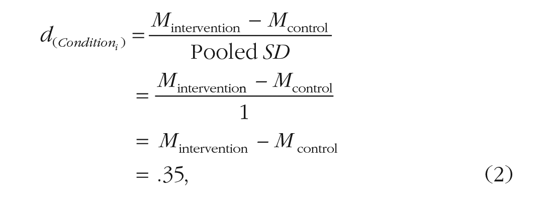
\begin{array}{l} d_{(C o n d i t i o n_{i})} = \frac{M_{i n t e r v e n t i o n} - M_{c o n t r o l}}{P o o l e d S D} \\ = \frac{M_{i n t e r v e n t i o n} - M_{c o n t r o l}}{1} \\ = M_{i n t e r v e n t i o n} - M_{c o n t r o l} \\ = . 35, \end{array}

(2)

where M_intervention and M_control represent the standardized mean in the intervention group and control group, respectively.

You now wonder how many participants are needed to detect such a median-sized main effect with a statistical power of 1 – β = 0.80 (i.e., if the effect exists, there is an 80% chance of detecting a true positive) using a two-tailed test with an α of .05 (i.e., if the effect does not exist, there is a 5% risk of detecting a false positive). To calculate the required N, you enter the three key parameters (expected d, target power, α) in G*Power, which uses a formula very similar to the following:²

\begin{array}{l} N = \frac{4 \times {(Z_{1 - α / 2 = . 025} + Z_{1 - β = . 80})}^{2}}{d_{{(C o n d i t i o n_{i})}^{2}}} \\ = \frac{4 \times {(1.96 + 0.84)}^{2}}{{0.35}^{2}} \\ = 256, \end{array}

(3)

where Z_1-α/2=.025 = 1.96 and Z_1-β=.80 = 0.84 are the critical Z values associated with a two-tailed test with α = .05 and 1 – β = 0.80, respectively.

Simply put, assuming that your intervention works as expected, a sample size of 256 participants will give you an 80% probability to observe a median-sized (or larger) effect of Condition_i with p < .05.

Calculating the required sample size to detect an interaction effect of a typical size

Now imagine you believe that your intervention should benefit only women, not men.³ You are planning to use a 2 × 2 factorial design to test the following hypothesis: “Compared with women in the control group, women in the intervention group report higher levels of well-being; for men, there is no difference between the two conditions.” To test your hypothesis, you will use the multiple linear regression below:

{Well-being}_{i} = B_{0} + B_{1} \times {Condition}_{i} + B_{2} \times {Gender}_{i} + B_{3} \times {Condition}_{i} \times {Gender}_{i} + e_{i},

(4)

where Gender_i = −0.5 for men and +0.5 for women.

To plan your study efficiently, you must again begin by determining the expected effect size of Condition_i × Gender_i interaction. In this situation, you may feel it is reasonable to use the same generic value of d = 0.35 used above to describe an interaction effect of typical size. Then, because you now have a 2 × 2 instead of a two-group design, it may seem logical to double the sample size (for examples of recent articles following this reasoning, see Majer et al., 2022; Tepe & Byrne, 2022; Y. Wang & Xie, 2021). However, this would be a mistake.

The reason why this is a mistake is simple: Contrary to the Cohen’s d of a main effect in a two-group design, the Cohen’s d of an interaction in a 2 × 2 design should not be seen as a difference between means but as a difference between subdifferences. Assuming equal sample sizes and a SD = 1 for each of your subgroups, the calculation corresponds to the difference between (a) the subdifference between M_{intervention♀} and M_control♀ for women [the simple slope $d_{[C o n d i t i o n_{i}] ♀}$ ] and (b) the subdifference between M_{intervention♂} and M_control♂ for men [the simple slope $d_{(C o n d i t i o n_{i}) ♂}$ ]:

\begin{array}{l} d_{(C o n d i t i o n_{i} \times G e n d e r_{i})} = \frac{(M_{i n t e r v e n t i o n ♀} - M_{c o n t r o l ♀}) - (M_{i n t e r v e n t i o n ♂} - M_{c o n t r o l ♂})}{2 \times P o o l e d S D} \\ = \frac{d_{(C o n d i t i o n_{i}) ♀} - d_{(C o n d i t i o n_{i}) ♂}}{2} . \end{array}

(5)

Because the effect size of an interaction is derived from the effect sizes of its simple slopes, it is not reasonable to expect the effect size of the Condition_i × Gender_i interaction to be as high as d = 0.35. Indeed, given that the simple slope for men is null, such an interaction would involve an unusually large simple slope for women of $d_{(C o n d i t i o n_{i}) ♀}$ = 0.70:

\begin{array}{l} d_{(C o n d i t i o n_{i} \times G e n d e r_{i})} = \frac{d_{(C o n d i t i o n_{i}) ♀} - d_{(C o n d i t i o n_{i}) ♂}}{2} \\ = \frac{0.70 - 0.00}{2} \\ = 0.35 . \end{array}

(6)

In this case, it would be more reasonable to expect the effect size of the Condition_i × Gender_i interaction to be d = 0.175 because such an interaction would this time involve a median simple slope for women of $d_{(C o n d i t i o n_{i})}$ = 0.35.

\begin{array}{l} d_{(C o n d i t i o n_{i} \times G e n d e r_{i})} = \frac{d_{(C o n d i t i o n_{i}) ♀} - d_{(C o n d i t i o n_{i}) ♂}}{2} \\ = \frac{0.35 - 0.00}{2} \\ = 0.175 . \end{array}

(7)

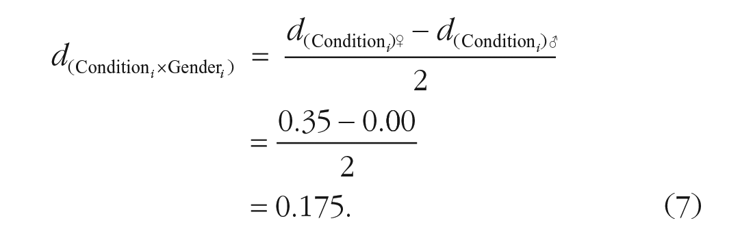
From there, you can use Equation 3 to calculate the required N to detect an interaction effect of d = 0.175 with a statistical power of .80 using a two-tailed test with α = .05. You will realize that you do not need a sample twice as large but 4 times as large as the sample used in the first case, that is, N = 1,024 participants.

\begin{array}{l} N = \frac{4 \times {(Z_{1 - α / 2 = . 025} + Z_{1 - β = . 80})}^{2}}{d_{{(C o n d i t i o n_{i} \times G e n d e r_{i})}^{2}}} \\ = \frac{4 \times {(1.96 + 0.84)}^{2}}{{0.175}^{2}} \\ = 1, 024 . \end{array}

(8)

Although this example is only one of many possible interactions, it illustrates the danger of relying on a generic value to define the expected effect size of an interaction (e.g., believing that an interaction of a typical size will always be d = 0.35). A less error-prone approach is to define the expected effect sizes of the simple slopes (e.g., a median simple slope of d = 0.35 combined with a null simple slope of d = 0.00) and work from there to determine the expected effect size of the interaction and the required sample size. In the next section, we propose a taxonomy of interactions that will allow us to provide comprehensive sample-size recommendations.

A taxonomy of 12 types of interactions

Now, we introduce an intuitive taxonomy of 12 types of interactions based on two criteria: (a) the expected shape of the interaction (based on the signs of the simple slopes) and (b) the expected sizes of the simple slopes (based on the values of the simple slopes). We give the required sample size to detect each interaction with adequate power.

Criterion 1. What is the expected shape of my interaction?

The literature typically defines three basic shapes of interaction: (a) a reversed interaction, (b) a fully attenuated interaction, and (c) a partially attenuated interaction (for related distinctions, see Baranger et al., 2022; Blake & Gangestad, 2020; Brysbaert, 2019; Giner-Sorolla, 2018; Lakens & Caldwell, 2021; Ledgerwood, 2019; Perugini et al., 2018).

First, a reversed interaction (also known as a “crossover interaction” or “reversal of the effect”) involves simple slopes that go in opposite directions (see Fig. 1, left). For instance, joining (vs. leaving) a group that one holds in high esteem increases life satisfaction, whereas joining (vs. leaving) a group that one holds in low esteem decreases life satisfaction (DeMarco & Newheiser, 2019).

Fig. 1.

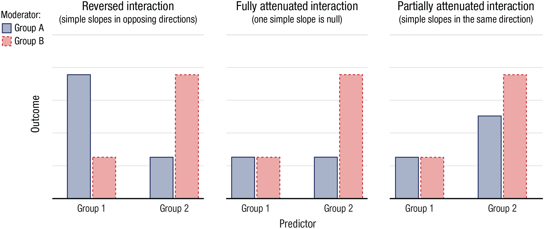
Example of a reversed interaction (left), a fully attenuated interaction (middle), and a partially attenuated interaction (right) in the context of a 2 (Predictor: Group 1 vs. Group 2) × 2 (Moderator: Group A vs. Group B) design. These are just three examples of reversed, fully attenuated, and partially attenuated interactions; other configurations are possible. For the reversed interaction, the main effects are set to zero, resulting in a symmetrical pattern; if one of the main effects was nonzero, the pattern would be asymmetrical. As another example, for the fully attenuated interaction, the two main effects are equal in size and positive, resulting in an ordinal interaction (the crossover of predicted values is at the boundary); if one of the main effects was negative, the interaction would become dis-ordinal ((Widaman et al., 2012).

Second, a fully attenuated interaction (also known as a “knockout interaction” or “elimination of the effect”) involves a simple slope that goes in one direction and a simple slope that is null (see Fig. 1, middle). For instance, students from lower socioeconomic backgrounds benefit from having a growth mindset, whereas students from higher socioeconomic backgrounds do not (Sisk et al., 2018).

Third, a partially attenuated interaction (also known as a “spreading interaction” or “attenuation of the effect”) involves simple slopes that go in the same direction but for which one slope is steeper than the other (see Fig. 1, right). For instance, middle-aged individuals who are less educated are more likely to be depressed, whereas in older individuals, the link between education and depression persists but is weaker (a trend known as the “age-as-leveler pattern”; Abrams & Mehta, 2019).

Criterion 2. What are the expected effect sizes of my simple slopes?

In an ideal world, researchers would always base their expectations for effect size on prior, high-powered, preregistered studies. However, researchers often test new hypotheses for which no such studies are available, leaving them with only a vague idea of the effect size in the population. Consequently, researchers often resort to using Cohen’s (1965) benchmarks (e.g., when using G*Power), which equate small, medium, and large effects to standardized mean differences of d = 0.20, 0.50, and 0.80, respectively (see Equation 2). Although these benchmarks are widely used today, Cohen (1988) himself recognized that they offer “no more reliable a source than intuition” and argued that “with the accumulation of experience, [these benchmarks] may well require revision (I suspect downward)” (p. 478).

Many scholars have discussed substituting Cohen’s classic benchmarks for empirically derived benchmarks (Brysbaert, 2019; Funder & Ozer, 2019; Hemphill, 2003). To this end, Gignac and Szodorai (2016) gathered correlation coefficients from 87 meta-analyses in social/personality psychology and established that the 25th, 50th, and 75th percentiles roughly corresponded to Cohen’s ds of 0.20, 0.40, and 0.60, respectively (see also Fraley & Marks, 2007; Lovakov & Agadullina, 2021; Richard et al., 2003). However, effect sizes from nonpreregistered studies are inflated by 2 to 5 times because of publication bias (Camerer et al., 2018; Ebersole et al., 2020; Klein et al., 2018), and these meta-analytically derived benchmarks are likely overestimations (Correll et al., 2020).

More recently, Schäfer and Schwarz (2019) gathered effect sizes from 93 randomly selected preregistered studies in psychology and found a slightly lower median effect size of about d = 0.35. Importantly, the authors documented significant variation in effect sizes among subdisciplines and study designs, indicating that there are no universally applicable benchmarks (see also Adachi & Willoughby, 2015; Flora, 2020; Lakens, 2013). Despite this limitation, we suggest that the following empirically derived benchmarks may be useful heuristic descriptions of relatively small, median, and relatively large effects: d = 0.20, d = 0.35, and d = 0.50, respectively (for correspondences with other types of estimates, see Table 1). These benchmarks can be used to quantify archetypal effect sizes or to define the smallest effect size of interest (Anvari & Lakens, 2021). For instance, d = 0.20 might sometimes be considered as the minimum effect size of theoretical or practical significance.

Table 1.

Empirically Derived Benchmarks Used in the Present Article

	Cohen’s d	Cohen’s f	Pearson’s r	η²_p
Smaller	0.20	0.10	.10	.01
Median	0.35	0.175	.17	.03
Larger	0.50	0.25	.24	.06

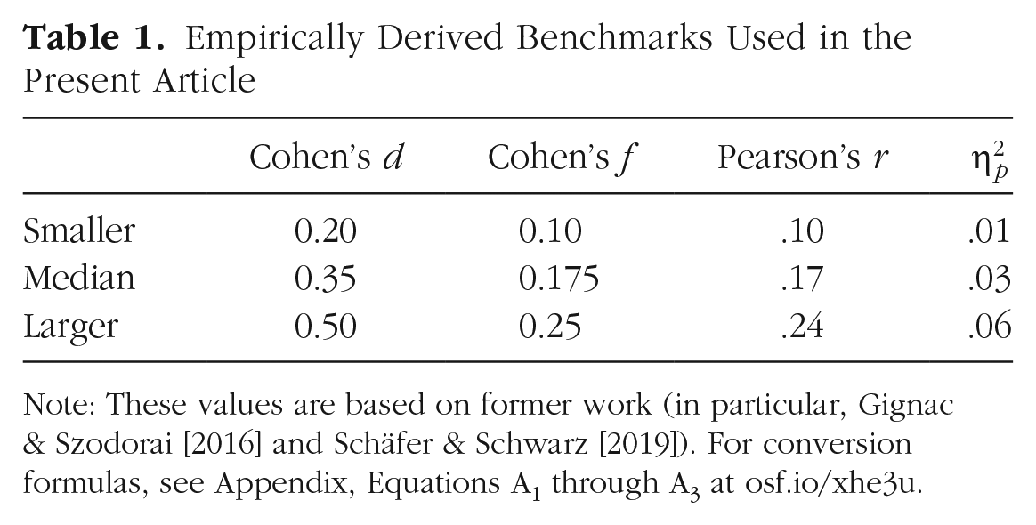
Note: These values are based on former work (in particular, Gignac & Szodorai [2016] and Schäfer & Schwarz [2019]). For conversion formulas, see Appendix, Equations A₁ through A₃ at osf.io/xhe3u.

12 types of interactions

Description of the taxonomy

As is shown in Table 2, our taxonomy covers interactions involving any combination of median (d = 0.35), smaller (d = 0.20), and larger (d = 0.50) simple slopes. This encompasses the following:

Table 2.

Taxonomy of 12 Possible Types of Interactions as a Function of Shape (Criterion 1) and Expected Effect Sizes of Simple Slopes (Criterion 2)

Criterion 1Shape	Criterion 2Expected effect sizes (Cohen’s d)				Overall interaction effect size	Total required sample size
Criterion 1Shape	Simple Slope 1		Simple Slope 2		Overall interaction effect size	Power = .80	Power = .90	Power = .95
Reversed	+0.20	(smaller)	−0.20	(smaller)	0.20	N = 784	N = 1,051	N = 1,300
Reversed	+0.20	(smaller)	−0.35	(median)	0.28	N = 415	N = 556	N = 687
Reversed	+0.20	(smaller)	−0.50	(larger)	0.35	N = 256	N = 343	N = 424
Reversed	+0.35	(median)	−0.35	(median)	0.35	N = 256	N = 343	N = 424
Reversed	+0.35	(median)	−0.50	(larger)	0.43	N = 174	N = 233	N = 288
Reversed	+0.50	(larger)	−0.50	(larger)	0.50	N = 125	N = 168	N = 208
Fully attenuated	+0.20	(smaller)	0.00	(null)	0.10	N = 3,136	N = 4,204	N = 5,198
Fully attenuated	+0.35	(median)	0.00	(null)	0.18	N = 1,024	N = 1,373	N = 1,697
Fully attenuated	+0.50	(larger)	0.00	(null)	0.25	N = 502	N = 673	N = 832
Partially attenuated	+0.20	(smaller)	+0.35	(median)	−0.08	N = 5,575	N = 7,474	N = 9,241
Partially attenuated	+0.20	(smaller)	+0.50	(larger)	−0.15	N = 1,394	N = 1,869	N = 2,310
Partially attenuated	+0.35	(median)	+0.50	(larger)	−0.08	N = 5,575	N = 7,474	N = 9,241

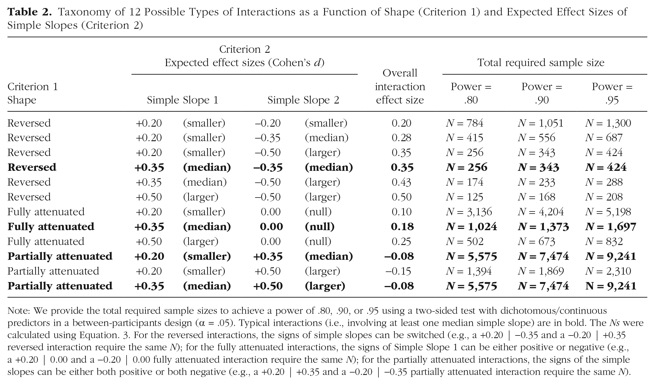
Note: We provide the total required sample sizes to achieve a power of .80, .90, or .95 using a two-sided test with dichotomous/continuous predictors in a between-participants design (α = .05). Typical interactions (i.e., involving at least one median simple slope) are in bold. The Ns were calculated using Equation. 3. For the reversed interactions, the signs of simple slopes can be switched (e.g., a +0.20 | −0.35 and a −0.20 | +0.35 reversed interaction require the same N); for the fully attenuated interactions, the signs of Simple Slope 1 can be either positive or negative (e.g., a +0.20 | 0.00 and a −0.20 | 0.00 fully attenuated interaction require the same N); for the partially attenuated interactions, the signs of the simple slopes can be either both positive or both negative (e.g., a +0.20 | +0.35 and a −0.20 | −0.35 partially attenuated interaction require the same N).

Six reversed interactions: The typical reversed interaction is the “+0.35|−0.35 reversed interaction,” which involves a median simple slope that goes in one direction (e.g., d = +0.35) and a median simple slope that goes in another direction (e.g., d = −0.35). Note that the order of the signs is arbitrary, given that a +0.35|−0.35 and a −0.35|+0.35 interaction have the same overall effect size of|d|= 0.35, which is equivalent to a median-sized main effect.

Three fully attenuated interactions: The typical fully attenuated interaction is the “+0.35|0.00 fully attenuated interaction,” which involves a median simple slope that goes in either direction (e.g., d = +0.35) and a null simple slope (d = 0.00). Note that the sign of the nonnull simple slope is arbitrary, given that a +0.35|0.00 and a −0.35|0.00 interaction have the same overall effect size of |d|= 0.175, which is half the size of a median-sized main effect.

Three partially attenuated interactions: The typical partially attenuated interactions are the “+0.20| +0.35” or the “+0.35|+0.50 partially attenuated interaction,” which involve a simple slope that goes in one direction (e.g., d = +0.20) and a larger simple slope that goes in the same direction (e.g., d = +0.35). Note that the common sign of the simple slopes is arbitrary, given that a −0.20|−0.35 and a −0.35|−0.50 interaction have the same overall effect size of|d|= 0.075, which is nearly 5 times smaller than a median-sized main effect.

Sample-size recommendations in between-participants designs and assumptions

In Table 2, we provide the required sample sizes to achieve power of .80, 90, or .95 when using a two-tailed test with α = .05 to detect each of the 12 interactions in 2 × 2 designs. The values of .80 and .90 are commonly used as lower limits for acceptable statistical power (Cohen, 1988), whereas .95 is a more stringent standard that may be useful in certain circumstances, such as when planning an exact replication (Hedges & Schauer, 2019).

These required sample sizes can be used as case-sensitive recommendations provided that the usual assumptions of linear regression are met: approximate multivariate normality (O’Connor, 2006), homogeneity of variance across subgroups (Overton, 2001), independence of residual error (Arend & Schäfer, 2019), and lack of severe multicollinearity (Shieh, 2010). However, in the context of interaction, two additional assumptions deserve particular attention (for relevant research, see Aguinis, 1995; Aguinis & Gottfredson, 2010; Jaccard et al., 2003; McClelland & Judd, 1993).

First, equal sample sizes are expected across subgroups. In our introductory example, this means having the same number of women and men in each condition. When this assumption is violated, the power to detect the interaction decreases, albeit only slightly. For instance, when the ratio is 2:1 instead of 1:1 (e.g., twice the number of women compared with men), power is reduced by approximately 5%. However, when the ratio is 9:1, power is reduced by 33% (Stone-Romero et al., 1994).

Second, measurement error should be zero. In our introductory example, regarding the moderator, this means that 100% of the participants are expected to report their gender without error (e.g., selecting the wrong response option). When this assumption is violated, the power to detect the interaction decreases in proportion to the degree of error: For instance, if 95% of the participants correctly reported their gender, the expected effect size used in the power analysis should be adjusted with d_adjusted = d × .95 (Blake & Gangestad, 2020). Note that our benchmarks, which are empirically derived from actual studies with measurement error, already take this into account (meaning if you manage to enhance reliability, you can use a larger expected effect size).

Anticipating two criticisms

Two potential arguments can be made against our taxonomy. First, one could argue that interactions with different shapes may have the same overall effect size, calling into question the relevance of the concept of “shape.” For example, reversed, fully attenuated, and partially attenuated interactions could all theoretically have an effect size of d = 0.35 and require the same N to reach power = .80. However, we find this argument misleading because reversed interactions with d = 0.35 involve median-sized simple slopes and are therefore relatively common, while attenuated interactions with d = 0.35 involve huge simple slopes and are almost never encountered.

Second, one can argue that the 12 interactions correspond to specific combinations of interactive and main effects, calling into question the importance of simple slopes. For instance, a fully attenuated interaction +0.35 |0.00 corresponds to a combination of interactive and main effects of ds = 0.175. However, we also find this argument irrelevant because researchers testing interactions do not typically think in terms of specific combinations of interactive and main effects. Rather, they hypothesize interaction patterns, making it practical to think about the relative sizes and signs of their expected simple slopes.

In the first part of this article, we showed that the required sample size to detect interactions is often larger than one would intuitively estimate, especially for attenuated interactions (for related research, see Bakker et al., 2016). In the second part, we report the findings of a preregistered metastudy showing that most studies testing interactions are indeed underpowered, and then we describe the results from simulations testing three approaches to increase power without increasing sample size.

How to Achieve Sufficient Power to Detect Interactions

A preregistered metastudy on power-analysis practices

In the second part of this article, we begin by describing the findings from a preregistered metastudy that examined the power analysis and research practices used in testing interaction hypotheses. We aimed to build a sample of relevant studies from approximately 100 articles⁴ published in 10 influential psychology journals. We sought to answer three research questions:

Research Question 1: What is the proportion of studies testing attenuated interactions (the most difficult to detect)?

Research Question 2: What is the proportion of studies using an adequate power analysis?

Research Question 3: What is the median statistical power of the studies?

Method

The study was preregistered (any deviation from the preregistered protocol is noted). The eligibility criteria, the preregistration, the coding sheets, the raw data set, and the Stata scripts to reproduce the findings can be found at https://osf.io/xh5tc/. We report how we determined our sample size, all data exclusions, all manipulations, and all measures in the metastudy.

Eligibility criteria and rationales

We focused on articles that met five eligibility criteria (for the detailed list, see Table S1 in the Supplemental Material). First, we focused on articles in which an interaction hypothesis was formulated a priori (Criterion 1) because NHST is mainly appropriate for confirmatory and not exploratory analysis (Wagenmakers et al., 2012; but see Rubin, 2017). Moreover, we focused on articles testing first-order interactions (Criterion 2) because second-order interactions correspond to a difference between differences of subdifferences and are notoriously harder to detect (Dawson & Richter, 2006). Finally, we focused on articles using a between-participants design (Criterion 3) and a regular regression framework (including analysis of variance [ANOVA]; Criterion 4) with a one-degree-of-freedom test (Criterion 5). The reason for these foci was that within-participants designs, nonlinear functions, multilevel modeling, polytomous variables, and so on all involve different formulas for statistical power calculations (see Brysbaert, 2019; Demidenko, 2008; Domingue et al., 2022; Mathieu et al., 2012). However, we will later show how mixed designs and planned-contrast analysis can be used to increase power.

Article selection and data extraction

Our study procedure consisted of three steps (for a flowchart detailing these steps and the number of articles and studies, see Fig. 2).

Fig. 2.

Flowchart depicting the three steps of the article-selection and data-extraction procedure.

Step 1: search strategy

In June 2021, we sampled articles from 10 top-tier empirical journals in general, social, and/or personality psychology (for the list of these journals and their characteristics, see Table 3). The median Journal Impact Factor Percentile was 85th, meaning that the typical journal in our data set was in the top 15% of its category (Clarivate Analytics, 2021). For each journal, we used PsycINFO to identify the 100 most recent articles containing the words “moderat*” or “interact*” (in any field). At the end of Step 1, our sample comprised K₁ = 10 (journals) × 100 (articles) = 1,000 articles.

Table 3.

List of the 10 Journals With Their Journal Impact Factor Percentile, the Number of Articles k at Each Intermediary Step, and the Number of Articles k and Studies n at the End of the Final Step

	Years	JIF perc.	Step 1 k	Step 2a k	Step 2b k	Step 3 n
JPSP	2021–2022	94th	100	20	9	21
PS	2019–2021	93rd	100	20	6	18
SPPS	2019–2021	92nd	100	20	9	12
EJP	2017–2019	91st	100	11	3	8
JP	2018–2020	85th	100	21	10	14
JESP	2020–2021	85th	100	23	9	20
JEP:G	2020–2021	82nd	100	26	6	8
PSPB	2021	84th	100	21	11	21
BJSP	2020–2021	80th	100	20	9	15
EJSP	2019–2021	73rd	100	20	10	22
Total	2017–2022	Median = 85	K = 1,000	K = 202	K = 82	N = 159

Note: Step 1 = search strategy; Step 2a = screening abstract and title; Step 2b = data extraction; Step 3 = data extraction; JIF perc. = Journal Impact Factor Percentile (JIF perc. transforms the rank in category by JIF into a percentile value, thereby allowing us to take the category of the journal into account); JPSP = Journal of Personality and Social Psychology; PS = Psychological Science; SPPS = Social Psychological and Personality Science; EJP = European Journal of Personality; JP = Journal of Personality; JESP = Journal of Experimental Social Psychology; JEP:G = Journal of Experimental Psychology: General; PSPB = Personality and Social Psychology Bulletin; BJSP = British Journal of Social Psychology; EJSP = European Journal of Social Psychology.

Step 2a: screening titles/abstracts

In July 2021, we gave two coders the titles and abstracts of the 1,000 articles. The coders were unaware of the specific purposes of the study. For each journal, they were asked to identify the 20 most recent articles that likely satisfied our five eligibility criteria. After training with articles from Social Psychological and Personality Science (SPPS), they coded the remaining articles independently using the following coding scheme: 0 = nonrelevant article, 1 = potentially relevant article. The interrater agreement, measured using Cohen’s kappa, was .70 (above our preregistered threshold of κ = .60), with a substantial percentage of agreement of 88.2% (Belur et al., 2021). Then, the two coders independently reviewed their disagreements and could change their responses (the remaining disagreements were resolved by discussion). At the end of Step 2a, our sample comprised 202 articles.⁵

Step 2b: screening full texts

In August 2021, we gave the two coders the full texts of the 202 articles. For each journal, the coders were asked to first identify the 10 most recent articles that satisfied Criteria 2 through 5 and then Criterion 1. After training with the articles from SPPS, they independently coded the remaining articles using the following coding scheme: 0 = nonrelevant article, 1 = relevant article. The interrater agreement was κ = .79, with a percentage of agreement of 90.7%. Disagreements were resolved by discussion. At the end of Step 2b, our sample comprised 82 articles.

Step 3: data extraction

In September 2021, we gave the two coders a data extraction spreadsheet (Table S2). For each of the 82 articles, the coders were asked to (a) identify the interaction hypothesis/es and specify its/their types (reversed, fully attenuated, or partially attenuated [Research Question 1]), (b) identify the power analysis/es and specify its/their characteristics (e.g., type, focus, whether the shape of the interaction was taken into account [Research Question 2]), and (c) collect the analytical sample size (for us to calculate power [Research Question 3]). After training with three articles from Psychological Science, they completed the spreadsheet independently. The mean interrater agreement for the categorical/numeric responses was .87, with an overall percentage of agreement for all questions of 82.0%. At the end of Step 3, our sample comprised 159 studies from 82 articles (≈ 2 studies per article). The sample size was somewhat below our target number of 100 articles. However, the articles were deemed representative of the current literature in that they covered a large proportion, if not most, of the target population of studies testing interactions published in the 10 chosen journals between 2017 and 2021.

Results

Research Question 1: What is the proportion of studies testing attenuated interactions?

About 85% of the studies tested attenuated-interaction hypotheses.

A total of 159 studies tested 194 interaction hypotheses. Seven studies were excluded from the analysis because the coders could not determine the shape of the hypothesized interactions. Among the 152 remaining studies, only 15% tested at least one reversed-interaction hypothesis, whereas 36% tested at least one fully attenuated interaction, and 52% tested at least one partially attenuated interaction (Fig. 3, left). Note that the percentages do not add up to 100% because one study could test multiple types of interaction hypotheses.

Fig. 3.

Proportion of studies as a function of the shape of the hypothesized interaction (pie chart, left) and number of studies as a function of the appropriateness of the power analysis (stacked bar chart, right). In the pie chart, the overlapping slices pertain to studies that include interaction hypotheses of different shapes.

Research Question 2: What is the proportion of studies using an adequate power analysis?

Less than 5% of the studies used an adequate power analysis.

Out of the 159 studies, 45% did not report a power/sensitivity analysis—specifically, 65 did not report any analysis, three did not specify the type of analysis, and three reported an incorrect “post hoc” power analysis (see Hoenig & Heisey, 2001). Another 20% reported a power/sensitivity analysis not focused on the interaction—specifically, 23 did not specify the focal effect, and nine focused on a main effect or another type of effect. Finally, another 32% reported a power or sensitivity analysis focused on the interaction but did not take the shape of the interaction into account. In sum, only 4% of the studies reported an adequate power analysis (Fig. 3, right).

Research Question 3: What is the median statistical power of the studies?

The overall median power to detect interactions of a typical size is .18.

For each hypothesis of each study, we used Equations 5 and A₄ (available at osf.io/xhe3u) to calculate the power afforded by the analytical sample size to detect the typical version of the interaction expected by the authors.⁶ For the studies testing a reversed interaction (n = 23),⁷ the power to detect a +0.35 |−0.35 reversed interaction was at or above .80 in 65% of the cases, and the median power was = .87. For the studies testing a fully attenuated interaction (n = 54), the power to detect a +0.35|0.00 fully attenuated interaction was at or above .80 in 19% of the cases, and the median power was .36. For the studies testing a partially attenuated interaction (n = 74), the power to detect a +0.35|+0.20 (or, equivalently, a +0.35|+0.50) partially attenuated interaction was at or above .80 in none of the cases, and the median power was .11. Overall, only 17% of the studies had a power at or above .80, and the median power was .18 (Fig.4, lower panel). If we repeat the analysis while focusing on larger versions of the hypothesized interactions (i.e., +0.50|−0.50, +0.50|0.00, and +0.50|+0.20), 27% of the studies had a power at or above .80, and the median power was .25.

Fig. 4.

Proportion of studies as a function of the power to detect the hypothesized interaction, assuming a typical size. We added spherical noise to the plotted markers to avoid overlap.

Discussion

Our metastudy shows that the majority of recently published studies testing interactions focus on attenuated interactions. Only a minority reported an adequate power analysis, and less than one in five studies has a sample size sufficient to detect an interaction of a typical size with a power of .80. This illustrates the fact that studies testing interactions are often underpowered, and in the next section, we present simulations aiming to test three approaches to increase power without increasing sample size.

Simulations testing ways to improve power for interactions

Now, we report the results from 877,500,000 simulations that served two aims: (a) producing the power curve for each of the 12 types of interactions (offering an empirical replication of the mathematically derived required sample size displayed in Table 2) and (b) testing three approaches to increase power without increasing sample size: one-tailed testing, mixed designs, and planned-contrast analysis.

Existing simulations

Several studies have used simulations to investigate the question of power when testing interactions (for pioneering work, see Champoux & Peters, 1987). In existing simulations, however, the size of the interaction in the population is often fixed across conditions (for exceptions, see Durand, 2013; Shieh, 2009), and the emphasis is put on important but very specific issues, such as the use of median split in multicollinearity contexts (Iacobucci et al., 2015; see also McClelland et al., 2015), the calculation of the product term in latent variable modeling (Chin et al., 2003; see also Goodhue et al., 2007), or the violation of the homoscedasticity assumption when sample sizes differ among subgroups (Alexander & DeShon, 1994; see also Aguinis & Stone-Romero, 1997). In our own simulations, we aimed to produce the power curve of the 12 interactions identified earlier and determine the extent to which these power curves could be flattened by the use of one-tailed testing, mixed designs, and planned contrast analysis.

Approach 1: preregistering the use of one-tailed testing

Most scientists using NHST use two-tailed tests (also called “two-sided” or “nondirectional” tests) with a canonical α of .05. This means that they place one half of their ^α (^α/₂ = .025) in the lower tail of the t distribution (testing whether an effect is less than zero) and the other half (^α/₂ = .025) in the upper tail (testing whether an effect is greater than zero; Wiley & Pace, 2015). To put it simply, if scientists are looking for an effect that does not exist in the population, they have a 2.5% chance of observing a negative effect with p < .05 and a 2.5% chance of observing a positive effect with p < .05 (the overall Type I error [false positive] rate is therefore 5%).

However, scientists using NHST often have an a priori hypothesis and could run a more powerful one-tailed test (also called “one-sided” or “directional” tests) with the same alpha of .05 (Knottnerus & Bouter, 2001). This involves placing all of the alpha (α = .05) in the tail of the t distribution corresponding to their hypothesis (the lower or upper tail, depending on whether they hypothesized a negative or positive effect) and refraining from interpreting any effect in the opposite direction (even if p < .05). In simpler terms, if a hypothesis is incorrect, there is a 5% chance of observing the hypothesized effect with p < .05 (maintaining an overall Type I error rate of 5%).

Statisticians have long recommended using one-tailed testing when a directional hypothesis is formulated and when an effect in the opposite direction would be psychologically meaningless and theoretically uninformative (Kimmel, 1957). Despite these conditions often being met, journal editors and reviewers tend to frown upon one-tailed testing. This reluctance may be due to the high prevalence of HARKing in the field (Motyl et al., 2017), which involves formulating a hypothesis after results are known (Kerr, 1998) and is likely influenced by hindsight bias (i.e., the “I-knew-it-all-along” effect; Nosek et al., 2018; see also Giner-Sorolla, 2012; Rubin, 2022). In such a context, one-tailed testing may be seen as overly liberal and a threat to cumulative science.

However, with the advent of preregistration (Van’t Veer & Giner-Sorolla, 2016; Wagenmakers et al., 2012) and registered reports (Chambers, 2013), it has become possible for researchers to record their hypothesis before running a study, thus effectively preventing HARKing (Lakens, 2019). We believe that whenever possible, researchers should create a preregistration in which they (a) clearly formulate their interaction hypothesis, (b) vow to not interpret an interaction in the opposite direction, and (c) plan to use one-tailed testing. We emphatically encourage this practice, believing it is both conceptually and pragmatically the best approach. A researcher registering an interaction hypothesis and the use of one-tailed rather than two-tailed testing (with α = .05) would need 21% fewer participants to reach a power of .80 (for the mathematical demonstration, see Appendix, Equations A_5a-c, at osf.io/xhe3u).

Approach 2: using mixed-participants designs

Despite the difficulty in comparing and calculating effect sizes across different designs (Lakens, 2013; Morris, 2008; Olejnik & Algina, 2003), combining between-participants and within-participants measures is usually considered an efficient way to increase statistical power (Lakens, 2022). This is because each participant from a study using two repeated measures does not provide one data point but two data points, reducing the error term by controlling for consistent individual differences (for related research, see Baker et al., 2021; Goulet & Cousineau, 2019). As a result, fewer participants are needed to detect the same type of effect while maintaining the same level of power, especially when the correlation between the within-participants measures is positive and large (Maxwell & Delaney, 2004).

Mixed-participants designs may have potential drawbacks. Participants may be more likely to discern the hypothesis, experience fatigue because of the increased length of the study, or be influenced by the order of presentation of the scales/conditions (Myers & Hansen, 2011). However, these drawbacks are arguably often outweighed by the benefits of increased statistical power. To illustrate, imagine a mixed-design study in which (a) the correlation between the measurements is ρ = .50 (a conservative estimate and less than the average correlation from existing [replication] studies; Brysbaert, 2019) and (b) the simple slope sizes of the within-participants variable is similar to what it would be in a between-participants design (despite the tendency for within-participants effects to be stronger; e.g., see Murphy et al., 2009). Given these assumptions, researchers testing an interaction and using a mixed design rather than a 2 × 2 between-participants design (with α = .05) would need 75% fewer participants to reach a power of .80 (for the mathematical demonstration, see Appendix, Equations A6_a-f, at osf.io/xhe3u). If they combined a mixed design with preregistered one-tailed testing, the researchers would need 80% fewer participants (1 − (1 − .75) × (1 − .21)).

Approach 3: preregistering the use of planned contrast analysis

The factorial approach is the default approach to testing interaction hypotheses. It involves regressing the outcome on the predictor, the moderator, and the product term, whose weights are as follows for the example used in the first part of the article:

	Control group		Intervention group
	Men	Women	Men	Women
Predictor (–1 = control, +1 = intervention)	−1	−1	+1	+1
Moderator (−1 = men, +1 = women)	−1	+1	−1	+1
Predictor × Moderator	+1	−1	−1	+1

As one can see, the weights of the product term form a cross (+1-1⤮+1-1), which makes it optimal for testing reversed interactions involving a negative simple slope for men (⁺¹↘_-1) and a positive simple slope for women (_-1↗⁺¹). However, these weights are suboptimal for testing other shapes of interaction, in particular, fully attenuated interactions.

An alternative approach is the planned-contrast approach (Rosenthal & Rosnow, 1985). In the case of a fully attenuated interaction, this approach involves concatenating (i.e., combining) the predictor and moderator variables and creating one planned and two orthogonal contrasts using Helmert coding (Rosnow & Rosenthal, 1991). The contrast weights could be as follows for the example used in the first part of the article:⁸

	Control group		Intervention group
	Men	Women	Men	Women
Planned contrast	−1	−1	−1	+3
Orthogonal Contrast 1	−1	+2	−1	0
Orthogonal Contrast 2	−1	0	+1	0

As one can see, the weights of the planned contrast form a left-angled triangle (_-1∆⁺_-³₁), corresponding to the hypothesized pattern and comparing women in the intervention group (+3) with participants in the three other subgroups (−1). The two orthogonal contrasts ensure that there is no residual difference between women in the control group and men (Orthogonal Contrast 1) or between men in the control group and men in the intervention group (Orthogonal Contrast 2).

To reject H₀, a significant planned contrast and nonsignificant orthogonal contrasts are needed (a likelihood ratio χ² could test for the joint significance of the orthogonal contrasts; Abelson & Prentice, 1997; Brauer & McClelland, 2005; Guggenmos et al., 2018). However, absence of evidence is not evidence of absence, and cautious analysts might want to use equivalence testing to ensure that the overall effect of the orthogonal contrasts is smaller than the smallest effect of interest (Lakens et al., 2018; Richter, 2016).

Importantly, some statisticians have argued that planned-contrast analysis offers excessive flexibility in data analysis (Ravenscroft & Buckless, 2017) and may not be suitable to test specific interaction patterns (see the debate between Abelson [1996] and Rosnow & Rosenthal [1996]). Thus, we recommend that authors preregister the use of contrast analysis and use it for testing only fully attenuated interactions in which three of the 2 × 2 means are expected to be the same. In such a case, researchers using planned-contrast analysis with Helmert coding rather than the orthodox factorial approach (with α = .05) would need 62% fewer participants to reach a power of .80 (for relevant work, see Perugini et al., 2018; for the mathematical demonstration, see Appendix, Equations A_7a-d, at osf.io/xhe3u). If they combined planned-contrast analysis with one-tailed testing, the researchers would need 70% fewer participants (1 − (1 − .62) × (1 − .21)).

Simulations testing the three approaches to increase power without increasing the N

Method

We used functions from the tidyverse, stats, and car packages in R-4.3.1 (Fox & Weisberg, 2018; R Core Team, 2013; Wickham et al., 2019) to simulate a total of 877,500,000 data sets with one continuous outcome variable, one categorical predictor, and one categorical moderator and generated power curves for the 12 interactions of our taxonomy while using (a) default conditions (between-participants design and a factorial approach) with two-tailed and one-tailed testing, (b) a mixed-participants design with two-tailed and one-tailed testing, and (c) planned-contrast analysis with two-tailed and one-tailed testing. The R scripts to reproduce the results are available at https://osf.io/xh5tc/.

For each interaction, we simulated 100,000 data sets with a sample size of n per condition, and we used an increment of n + 1 to identify the tipping points at which 80% and 90% of data sets returned significant tests with p < .05 (i.e., simulating 100,000 data sets with n = 100, another 100,000 with n = 101, another 100,000 with n = 102, etc.). In each case, this enabled us to identify the required Ns to achieve a power of .80 and .90, respectively (i.e., the most commonly used lower limits for acceptable power).

The population simple-slope sizes for the 12 interactions were d₁|d₂ = +0.20|−0.20, +0.20|−0.35, +0.20| −0.50, +0.35|−0.35, +0.35|−0.50, +0.50|−0.50, +0.20| 0.00, +0.35|0.00, +0.50|0.00, +0.20|+0.35, +0.20| +0.50, and +0.35|+0.50. To enable direct comparison across the four approaches, each data set was first sampled from a standard multivariate normal distribution and then adjusted using the mean vector $μ = [0 0 d_{1} d_{2}]'$ and the covariance matrices Σ relevant to each condition:

\begin{array}{l} F u l l y b e t w e e n d e s i g n M i x e d d e s i g n \\ Σ = [\begin{matrix} \begin{matrix} \begin{matrix} 1 \\ 0 \end{matrix} & \begin{matrix} 0 \\ 1 \end{matrix} \\ \begin{matrix} 0 \\ 0 \end{matrix} & \begin{matrix} 0 \\ 0 \end{matrix} \end{matrix} & \begin{matrix} \begin{matrix} 0 \\ 0 \end{matrix} & \begin{matrix} 0 \\ 0 \end{matrix} \\ \begin{matrix} 1 \\ 0 \end{matrix} & \begin{matrix} 0 \\ 1 \end{matrix} \end{matrix} \end{matrix}] Σ = [\begin{matrix} \begin{matrix} \begin{matrix} 1 \\ 0 \end{matrix} & \begin{matrix} 0 \\ 1 \end{matrix} \\ \begin{matrix} ρ \\ 0 \end{matrix} & \begin{matrix} 0 \\ ρ \end{matrix} \end{matrix} & \begin{matrix} \begin{matrix} ρ \\ 0 \end{matrix} & \begin{matrix} 0 \\ ρ \end{matrix} \\ \begin{matrix} 1 \\ 0 \end{matrix} & \begin{matrix} 0 \\ 1 \end{matrix} \end{matrix} \end{matrix}], \end{array}

(9)

where within-subjects correlations in the mixed design were set to ρ = .50, a conservative estimate that was well below the median value of ρ = .75 from replication studies (Brysbaert, 2019).⁹

In the default approach, for each d₁|d₂ combination and each n, we calculated the proportion of the 100,000 data sets for which a regression analysis using a factorial approach returned a significant interaction between the between-participants predictor and moderator. We repeated this for both two-tailed and one-tailed tests.

In the mixed-designs approach, for each d₁|d₂ combination and each N, we calculated the proportion of the 100,000 data sets for which a mixed analysis of variance returned a significant interaction between the between-participants predictor and the within-participants moderator. We repeated this for both two-tailed and one-tailed tests.

In the planned-contrast-analysis approach, we focused only on fully attenuated interactions, and we created a planned contrast (assigning weights of ^-1/₄|^-1/₄|⁺³/₄|^-1/₄ to the 2 × 2 cells of the interaction) and two orthogonal contrasts (using weights of ^-1/₃|^-1/₃|0|⁺²/₃| and ^-1/₂|⁺¹/₂| 0|0). For each of the three d₁ | d₂ combinations and each N, we calculated the proportion of the 100,000 data sets for which a regression analysis returned a significant planned contrast and a nonsignificant joint test of the orthogonal contrasts (using an omnibus postestimation two-tailed Wald test). We repeated this for both two-tailed and one-tailed tests.

Results

The simulation revealed two sets of findings. First, the mathematically derived required sample sizes for each of the 12 interactions calculated in the first part of the article were replicated using simulations: The required Ns to detect the interactions with a power of .80 ranged from 128 (to detect a +0.50|−0.50 reversed interaction) to 5,632 (to detect a +0.35|+0.50 partially attenuated interaction). Second, compared with the power curves of the default approach with two-tailed testing, (a) preregistering one-tailed tests require 21.3% and 18.5% fewer participants to reach a power of .80 and .90, respectively; (b) using a mixed design with ρ = .50 requires 74.6% and 74.7% fewer participants when using two-tailed testing and 80.1% and 79.4% when using one-tailed testing; and (c) preregistering planned-contrast analysis requires 62.6% and 59.4% fewer participants when using two-tailed testing and 70.1% and 66.3% when using one-tailed testing (for the required Ns, see Table 4; for the simulation-based power curves, see Fig. 5).

Table 4.

Overall Required Sample Sizes for the 12 Types of Interactions as a Function of Approach

	Simple Slope 1	Simple Slope 2	Default		Mixed design		Planned contrast
	Simple Slope 1	Simple Slope 2	Two-tailed	One-tailed	Two-tailed	One-tailed	Two-tailed	One-tailed
Power = .80	+0.20	−0.20	788	620	198	154
	+0.20	−0.35	416	328	106	84
	+0.20	−0.50	260	204	66	52
	+0.35	−0.35	260	204	66	52
	+0.35	−0.50	176	140	46	36
	+0.50	−0.50	128	100	34	26
	+0.20	0.00	3,124	2,476	786	624	1,172	940
	+0.35	0.00	1,028	812	258	202	384	304
	+0.50	0.00	504	396	128	100	188	152
	+0.20	+0.35	5,588	4,384	1,390	1,096
	+0.20	+0.50	1,396	1,100	352	276
	+0.35	+0.50	5,632	4,412	1,392	1,096
Power = .90	+0.20	−0.20	1,056	860	266	216
	+0.20	−0.35	556	456	142	114
	+0.20	−0.50	344	280	88	72
	+0.35	−0.35	344	280	88	72
	+0.35	−0.50	236	192	60	48
	+0.50	−0.50	172	140	44	36
	+0.20	0.00	4,224	3,436	1,060	854	1,716	1,424
	+0.35	0.00	1,376	1,120	344	284	556	464
	+0.50	0.00	676	548	170	138	276	228
	+0.20	+0.35	7,448	6,088	1,868	1,524
	+0.20	+0.50	1,856	1,524	468	382
	+0.35	+0.50	7,516	6,108	1,866	1,518

Fig. 5.

Simulation-based power curves for the 12 types of interactions as a function of approach. Power curves for the second half of the mixed-design approach were extrapolated.

Other ways to maximize power

In our simulation, we chose to focus on one-tailed testing, mixed designs, and planned-contrast analysis because they present minimal potential drawbacks. Although there are other approaches to increase power without increasing sample size, they often carry greater drawbacks. For instance, increasing sample homogeneity (Heidel, 2016), using instructional manipulation checks (Oppenheimer et al., 2009), or controlling for relevant covariates (Hernández et al., 2004) can enhance power but may also pose a threat to generalizability, alienate participants, or create spurious suppression effects, respectively.

However, as briefly mentioned in the first part of the article, an approach to maximizing power with little or no drawbacks is to increase the reliability of the outcome. Basically, when reliability increases, the effect size increases, resulting in increased power (implying that if your outcome is measured with higher than average reliability, the benchmarks used in this article may be underestimations). Heo et al. (2015) demonstrated that by increasing Cronbach’s α from the minimum acceptable level of .70 to a high value of .90, the power to detect an interaction in a mixed design can increase from approximately .40 to almost .90. Consequently, improving reliability by using validated scales instead of made-up scales, using multiple-item measures instead of single-item measures, or using multiple trials rather than just one can each be an extremely efficient way to increase power for detecting interactions.

A User-Friendly Web App to Conduct Power Analyses for Interactions

There are countless existing software and applications to run power analyses. Some are general and focus on the most common statistical tests (e.g., G*Power, Faul et al., 2007; PANGEA, Bartlett & Charles, 2021; the jpower module in Jamovi, Bartlett & Charles, 2021). Others are specific to certain statistical tests, such as multilevel regression (summary-statistics-based power for mixed-effects modeling, Murayama et al., 2022), structural equation modeling (pwrSEM, Y. A. Wang & Rhemtulla, 2021), and functional MRI study analyses (NeuroPower, Durnez et al., 2016).

Some applications enable one to run power analyses for interactions, such as InteractionPower (Baranger et al., 2022), Superpower (Lakens & Caldwell, 2021), or Power Analysis for 2 × 2 Factorial Interaction (White, 2018). Although these applications are useful, they may not always be intuitive. For instance, InteractionPower requires users to input the effect size of the interaction term as a correlation coefficient. Although some researchers will manage to calculate the expected size of their interaction correctly (e.g., using Equations 5 and A₂, available at osf.io/xhe3u), others may use generic benchmarks and enter an inappropriate value. Superpower may be more intuitive because it asks users to input the most common standard deviation and the raw means for each cell in the ANOVA. However, an even simpler approach would be to allow users to draw their interaction. Therefore, we have developed an application to run power analyses for interactions that requires only basic statistical knowledge and relies on a user-friendly graphical interface.

Introducing Int×Power

Int×Power is a user-friendly web app that enables researchers to easily draw their expected two-way interaction and produce the required overall sample size to achieve the target power of your choice. In addition, Int×Power enables researchers to employ approaches to maximize power (one-tailed testing, mixed designs, and planned-contrast analysis).

Int×Power is a JavaScript web app created using the React framework with Material UI. All libraries used are open source. The application is hosted at www.intxpower.com. The source code of the application is available on GitHub at https://github.com/ncheutin/INTxPower. A document presenting the underlying equation can be found on the OSF.

Quick tour of the web app

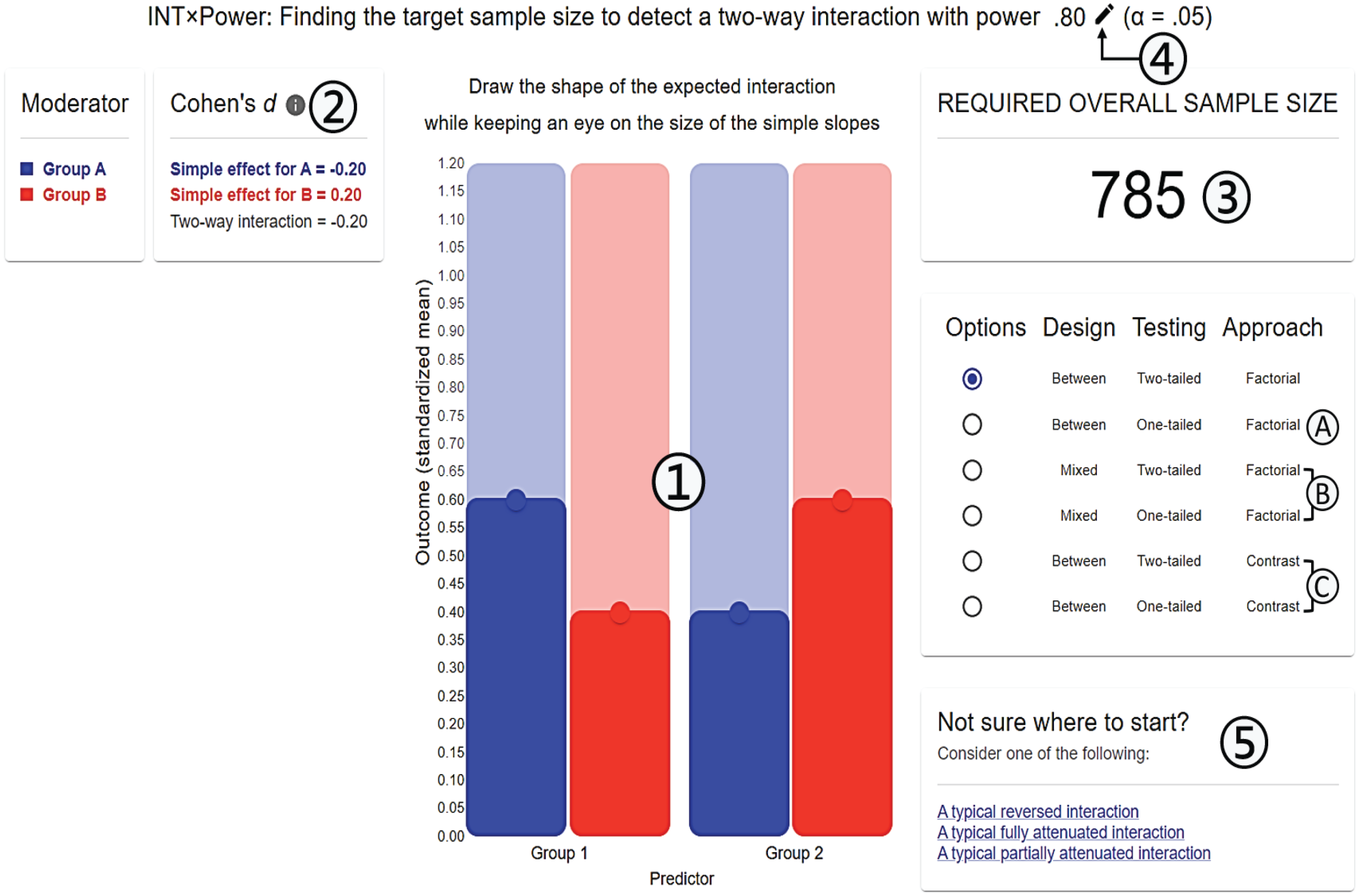
Figure 6 presents an annotated screenshot of Int×Power, showing the key components of the app. For a quick 1-min and 30-sec video tutorial, go to https://youtu.be/_ENvQF2aNmE.

Fig. 6.

Annotated screenshot of Int×Power showing the key components of the Web app. ➀ Users manipulate the 2 × 2 bars of their expected interaction. ➁ Users see the effect sizes of the simple slopes vary in real time. ➂ Users also see the required overall N to reach a power of .80 vary in real time. ➃ Users can change the default target power of .80 for any value. ➄ Users who are unsure where to start can automatically produce a bar chart representing an interaction of the expected shape and using the typical size.

The main equation used to calculate the required overall sample size is Equation 8, but this equation can be changed to apply to (a) one-tailed rather than two-tailed testing; (b) mixed-participants design rather than between-participants design, using two-tailed or one-tailed testing; and (c) planned-contrast approach with Helmert coding rather than factorial-design approach, using two-tailed or one-tailed testing (only for fully attenuated interactions).

Assumptions and future version(s)

Int×Power focuses on two-way interactions and relies on the same assumptions described in the first part of the article as well as sphericity and a common between-measurements correlation of ρ = .50 for mixed-participants designs. Although the interface uses dichotomous predictors, Int×Power can be applied to continuous predictors provided that measurement error does not differ between the two cases.

The version of the application is 1.0. We invite users to report bugs and request new features by sending an email to N. Sommet (updates to the source code will be documented on GitHub). Future version(s) of the app may allow users to calculate power for higher-order interactions, predictor/moderator with three categories or more, nonlinear regression such as logistic or Poisson regression, and so on. These changes will be the subject of further publications.

Supplemental Material

sj-docx-1-amp-10.1177_25152459231178728 – Supplemental material for How Many Participants Do I Need to Test an Interaction? Conducting an Appropriate Power Analysis and Achieving Sufficient Power to Detect an Interaction

Supplemental material, sj-docx-1-amp-10.1177_25152459231178728 for How Many Participants Do I Need to Test an Interaction? Conducting an Appropriate Power Analysis and Achieving Sufficient Power to Detect an Interaction by Nicolas Sommet, David L. Weissman, Nicolas Cheutin and Andrew J. Elliot in Advances in Methods and Practices in Psychological Science

Footnotes

Acknowledgements

We thank Adrien Anex and Umberto Cauzo for their help with data collection and David Baranger, Marcello Gallucci, and Dominique Muller for their feedback on the article.

Transparency

Action Editor: Yasemin Kisbu-Sakarya

Editor: David A. Sbarra

Author Contribution(s)

Nicolas Sommet: Conceptualization; Data curation; Formal analysis; Investigation; Methodology; Writing – original draft; Writing – review & editing.

David L. Weissman: Conceptualization; Data curation; Formal analysis; Methodology; Writing – original draft; Writing – review & editing.

Nicolas Cheutin: Software.

Andrew J. Elliot: Conceptualization; Methodology; Writing – review & editing.

ORCID iD

Nicolas Sommet

Supplemental Material

Additional supporting information can be found at

Notes

References

Abelson

R. P.

(1996). Vulnerability of contrast tests to simpler interpretations: An addendum to Rosnow and Rosenthal. Psychological Science, 7(4), 242–246.

Abelson

R. P.

Prentice

D. A.

(1997). Contrast tests of interaction hypothesis. Psychological Methods, 2(4), 315–328.

Aberson

C. L.

(2019). Applied power analysis for the behavioral sciences. Routledge.

Abrams

L. R.

Mehta

N. K.

(2019). Changes in depressive symptoms over age among older Americans: Differences by gender, race/ethnicity, education, and birth cohort. SSM-Population Health, 7, Article 100399. https://doi.org/10.1016/j.ssmph.2019.100399

Adachi

Willoughby

(2015). Interpreting effect sizes when controlling for stability effects in longitudinal autoregressive models: Implications for psychological science. European Journal of Developmental Psychology, 12(1), 116–128.

Aguinis

(1995). Statistical power problems with moderated multiple regression in management research. Journal of Management, 21(6), 1141–1158.

Aguinis

Gottfredson

R. K.

(2010). Best-practice recommendations for estimating interaction effects using moderated multiple regression. Journal of Organizational Behavior, 31(6), 776–786.

Aguinis

Stone-Romero

E. F.

(1997). Methodological artifacts in moderated multiple regression and their effects on statistical power. Journal of Applied Psychology, 82(1), 192–206.

Aiken

L. S.

West

S. G.

Reno

R. R.

(1991). Multiple regression: Testing and interpreting interactions. Sage.

10.

Alexander

R. A.

DeShon

R. P.

(1994). Effect of error variance heterogeneity on the power of tests for regression slope differences. Psychological Bulletin, 115(2), 308–314.

11.

Altmejd

Dreber

Forsell

Huber

Imai

Johannesson

Kirchler

Nave

Camerer

(2019). Predicting the replicability of social science lab experiments. PLOS ONE, 14(12), Article e0225826. https://doi.org/10.1371/journal.pone.0225826

12.

Anvari

Lakens

(2021). Using anchor-based methods to determine the smallest effect size of interest. Journal of Experimental Social Psychology, 96, Article 104159. https://doi.org/10.1016/j.jesp.2021.104159

13.

Arend

M. G.

Schäfer

(2019). Statistical power in two-level models: A tutorial based on Monte Carlo simulation. Psychological Methods, 24(1), 1–19.

14.

Baker

D. H.

Vilidaite

Lygo

F. A.

Smith

A. K.

Flack

T. R.

Gouws

A. D.

Andrews

T. J.

(2021). Power contours: Optimising sample size and precision in experimental psychology and human neuroscience. Psychological Methods, 26(3), 295–314.

15.

Bakker

Hartgerink

C. H.

Wicherts

J. M.

van der Maas

H. L.

(2016). Researchers’ intuitions about power in psychological research. Psychological Science, 27(8), 1069–1077.

16.

Baranger

Finsaas

Goldstein

Vize

Lynam

Olino

(2022). InteractionPoweR: Power analyses for interaction effects in cross-sectional regressions. PsyArXiv. https://doi.org/10.31234/osf.io/5ptd7

17.

Bartlett

J. E.

Charles

(2021). Power to the people: A beginner’s tutorial to power analysis using Jamovi. PxyArXiv. https://doi.org/10.31234/osf.io/bh8m9

18.

Belur

Tompson

Thornton

Simon

(2021). Interrater reliability in systematic review methodology: Exploring variation in coder decision-making. Sociological Methods & Research, 50(2), 837–865.

19.

Blake

K. R.

Gangestad

(2020). On attenuated interactions, measurement error, and statistical power: Guidelines for social and personality psychologists. Personality and Social Psychology Bulletin, 46(12), 1702–1711.

20.

Brauer

McClelland

(2005). L’utilisation des contrastes dans l’analyse des données: Comment tester les hypothèses spécifiques dans la recherche en psychologie? [The use of contrasts in data analysis: How to test specific hypotheses in psychological research]. l’Année Psychologique, 105(2), 273–305.

21.

Bredan

(2020). Conducting publishable research under conditions of severely limited resources. Libyan Journal of Medicine, 15(1), Article 1688126. https://doi.org/10.1080/19932820.2019.1688126

22.

Brysbaert

(2019). How many participants do we have to include in properly powered experiments? A tutorial of power analysis with reference tables. Journal of Cognition, 2(1), Article 16. https://doi.org/10.5334/joc.72

23.

Button

K. S.

Ioannidis

J. P.

Mokrysz

Nosek

B. A.

Flint

Robinson

E. S.

Munafò

M. R.

(2013). Power failure: Why small sample size undermines the reliability of neuroscience. Nature Reviews: Neurosciences, 14(5), 365–376.

24.

Camerer

C. F.

Dreber

Holzmeister

T.-H.

Huber

Johannesson

Kirchler

Nave

Nosek

B. A.

Pfeiffer

(2018). Evaluating the replicability of social science experiments in Nature and Science between 2010 and 2015. Nature Human Behaviour, 2(9), 637–644.

25.

Chambers

C. D.

(2013). Registered reports: A new publishing initiative at Cortex. Cortex, 49(3), 609–610.

26.

Champely

Ekstrom

Dalgaard

Gill

Weibelzahl

Anandkumar

Ford

Volcic

De Rosario

(2017). pwr: Basic functions for power analysis. http://CRAN.R-project.org/package=pwr

27.

Champoux

J. E.

Peters

W. S.

(1987). Form, effect size and power in moderated regression analysis. Journal of Occupational Psychology, 60(3), 243–255.

28.

Chin

W. W.

Marcolin

B. L.

Newsted

P. R.

(2003). A partial least squares latent variable modeling approach for measuring interaction effects: Results from a Monte Carlo simulation study and an electronic-mail emotion/adoption study. Information Systems Research, 14(2), 189–217.

29.

Clarivate Analytics. (2021). InCites journal citation reports 2021. Erlbaum.

30.

Cohen

(1965). Some statistical issues in psychological research. In Wolman

B. B.

(Ed.), Handbook of clinical psychology (pp. 95–121). McGraw-Hill.

31.

Cohen

(1988). Statistical power analysis for the behavioral sciences. Routledge.

32.

Correll

Mellinger

McClelland

G. H.

Judd

C. M.

(2020). Avoid Cohen’s ‘small’, ‘medium’, and ‘large’ for power analysis. Trends in Cognitive Sciences, 24(3), 200–207.

33.

Cronbach

L. J.

(1987). Statistical tests for moderator variables: Flaws in analyses recently proposed. Psychological Bulletin, 102(3), 414–417.

34.

Dawson

J. F.

Richter

A. W.

(2006). Probing three-way interactions in moderated multiple regression: Development and application of a slope difference test. Journal of Applied Psychology, 91(4), 917–926.

35.

DeMarco

T. C.

Newheiser

A. K.

(2019). When groups do not cure: Group esteem moderates the social cure effect. European Journal of Social Psychology, 49(7), 1421–1438.

36.

Demidenko

(2008). Sample size and optimal design for logistic regression with binary interaction. Statistics in Medicine, 27(1), 36–46.

37.

Domingue

Kanopka

Trejo

Rhemtulla

Tucker-Drob

(2022). Ubiquitous bias & false discovery due to model misspecification in analysis of statistical interactions: The role of the outcome’s distribution and metric properties. Psychological Methods. Advance online publication. https://doi.org/10.1037/met0000532

38.

Durand

C. P.

(2013). Does raising type 1 error rate improve power to detect interactions in linear regression models? A simulation study. PLOS ONE, 8(8), Article e71079. https://doi.org/10.1371/journal.pone.0071079

39.

Durnez

Degryse

Moerkerke

Seurinck

Sochat

Poldrack

R. A.

Nichols

T. E.

(2016). Power and sample size calculations for fMRI studies based on the prevalence of active peaks. BioRxiv. https://doi.org/10.1101/049429

40.

Ebersole

C. R.

Mathur

M. B.

Baranski

Bart-Plange

D.-J.

Buttrick

N. R.

Chartier

C. R.

Corker

K. S.

Corley

Hartshorne

J. K.

IJzerman

Lazarević

L. B.

Rabagliati

Ropovik

Aczel

Aeschbach

L. F.

Andrighetto

Arnal

J. D.

Arrow

Babincak

. . . Nosek

B. A.

(2020). Many Labs 5: Testing pre-data-collection peer review as an intervention to increase replicability. Advances in Methods and Practices in Psychological Science, 3(3), 309–331. https://doi.org/10.1177/2515245920958

41.

Faul

Erdfelder

Lang

A.-G.

Buchner

(2007). G* Power 3: A flexible statistical power analysis program for the social, behavioral, and biomedical sciences. Behavior Research Methods, 39(2), 175–191.

42.

Flora

D. B.

(2020). Thinking about effect sizes: From the replication crisis to a cumulative psychological science. Canadian Psychology / Psychologie Canadienne, 61(4), 318–330.

43.

Fox

Weisberg

(2018). An R companion to applied regression. Sage.

44.

Fraley

R. C.

Marks

M. J.

(2007). The null hypothesis significance testing debate and its implications for personality research. In Robins

R. W.

Fraley

R. C.

Krueger

R. F.

(Eds.), Handbook of research methods in personality psychology (pp. 149–169). The Guilford Press.

45.

Fraley

R. C.

Vazire

(2014). The N-pact factor: Evaluating the quality of empirical journals with respect to sample size and statistical power. PLOS ONE, 9(10), Article e109019. https://doi.org/10.1371/journal.pone.0109019

46.

Funder

D. C.

Ozer

D. J.

(2019). Evaluating effect size in psychological research: Sense and nonsense. Advances in Methods and Practices in Psychological Science, 2(2), 156–168.

47.

Gelman

(2018). You need 16 times the sample size to estimate an interaction than to estimate a main effect. https://statmodeling.stat.columbia.edu/2018/03/15/need-16-times-sample-size-estimate-interaction-estimate-main-effect/

48.

Gignac

G. E.

Szodorai

E. T.

(2016). Effect size guidelines for individual differences researchers. Personality and Individual Differences, 102, 74–78.

49.

Giner-Sorolla

(2012). Science or art? How aesthetic standards grease the way through the publication bottleneck but undermine science. Perspectives on Psychological Science, 7(6), 562–571.

50.

Giner-Sorolla

(2018). Powering your interaction. https://approachingblog.wordpress.com/2018/01/24/powering-your-interaction-2

51.

Goodhue

Lewis

Thompson

(2007). Research note—Statistical power in analyzing interaction effects: Questioning the advantage of PLS with product indicators. Information Systems Research, 18(2), 211–227.

52.

Goulet

M.-A.

Cousineau

(2019). The power of replicated measures to increase statistical power. Advances in Methods and Practices in Psychological Science, 2(3), 199–213.

53.

Guggenmos

R. D.

Piercey

M. D.

Agoglia

C. P.

(2018). Custom contrast testing: Current trends and a new approach. The Accounting Review, 93(5), 223–244.

54.

Hedges

L. V.

Schauer

J. M.

(2019). More than one replication study is needed for unambiguous tests of replication. Journal of Educational and Behavioral Statistics, 44(5), 543–570.

55.

Heidel

R. E.

(2016). Causality in statistical power: Isomorphic properties of measurement, research design, effect size, and sample size. Scientifica (Cairo), 2016, Article 8920418. https://doi.org/10.1155/2016/8920418

56.

Hemphill

J. F.

(2003). Interpreting the magnitudes of correlation coefficients. American Psychologist, 58(1), 78–79.

57.

Heo

Kim

Faith

M. S.

(2015). Statistical power as a function of Cronbach alpha of instrument questionnaire items. BMC Medical Research Methodology, 15(1), Article 86. https://doi.org/10.1186/s12874-015-0070-6

58.

Hernández

A. V.

Steyerberg

E. W.

Habbema

J. D.

(2004). Covariate adjustment in randomized controlled trials with dichotomous outcomes increases statistical power and reduces sample size requirements. Journal of Clinical Epidemiology, 57(5), 454–460.

59.

Hoenig

J. M.

Heisey

D. M.

(2001). The abuse of power: The pervasive fallacy of power calculations for data analysis. The American Statistician, 55(1), 19–24.

60.

Iacobucci

Posavac

S. S.

Kardes

F. R.

Schneider

M. J.

Popovich

D. L.

(2015). Toward a more nuanced understanding of the statistical properties of a median split. Journal of Consumer Psychology, 25(4), 652–665.

61.

Jaccard

Turrisi

Jaccard

(2003). Interaction effects in multiple regression (Vol. 72). Sage.

62.

Kerr

N. L.

(1998). HARKing: Hypothesizing after the results are known. Personality and Social Psychology Review, 2(3), 196–217.

63.

Kimmel

H. D.

(1957). Three criteria for the use of one-tailed tests. Psychological Bulletin, 54(4), 351–353.https://doi.org/10.1037/h0046737

64.

Klein

R. A.

Vianello

Hasselman

Adams

B. G.

Adams

R. B.

Jr. Alper

Aveyard

Axt

J. R.

Babalola

M. T.

Bahník

. (2018). Many Labs 2: Investigating variation in replicability across samples and settings. Advances in Methods and Practices in Psychological Science, 1(4), 443–490.

65.

Knottnerus

J. A.

Bouter

L. M.

(2001). The ethics of sample size: Two-sided testing and one-sided thinking. Journal of Clinical Epidemiology, 54(2), 109–110.

66.

Kovacs

van Ravenzwaaij

Hoekstra

Aczel

(2022). Samplesizeplanner: A tool to estimate and justify sample size for two-group studies. Advances in Methods and Practices in Psychological Science, 5(1). https://doi.org/10.1177/25152459211054059

67.

Lakens

(2013). Calculating and reporting effect sizes to facilitate cumulative science: A practical primer for t-tests and ANOVAs. Frontiers in Psychology, 4, Article 863. https://doi.org/10.3389/fpsyg.2013.00863

68.

Lakens

(2019). The value of preregistration for psychological science: A conceptual analysis. Japanese Psychological Review, 62(3), 221–230.

69.

Lakens

(2022). Sample size justification. Collabra: Psychology, 8(1), Article 33267. https://doi.org/10.1525/collabra.33267

70.

Lakens

Caldwell

A. R.

(2021). Simulation-based power analysis for factorial analysis of variance designs. Advances in Methods and Practices in Psychological Science, 4(1). https://doi.org/10.1177/2515245920951503

71.

Lakens

Scheel

A. M.

Isager

P. M.

(2018). Equivalence testing for psychological research: A tutorial. Advances in Methods and Practices in Psychological Science, 1(2), 259–269.

72.

Ledgerwood

(2019). New developments in research methods. In Baumeister

R. F.

Finkel

E. J.

(Eds.), Advanced social psychology (pp. 39–61). Oxford University Press.

73.

Lovakov

Agadullina

E. R.

(2021). Empirically derived guidelines for effect size interpretation in social psychology. European Journal of Social Psychology, 51(3), 485–504.

74.

Majer

J. M.

Zhang

Höhne

B. P.

Trötschel

(2022). Give and take frames in shared-resource negotiations. Journal of Economic Psychology, 90, Article 102492. https://doi.org/10.1016/j.joep.2022.102492

75.

Mathieu

J. E.

Aguinis

Culpepper

S. A.

Chen

(2012). Understanding and estimating the power to detect cross-level interaction effects in multilevel modeling. Journal of Applied Psychology, 97(5), 951–966.

76.

Maxwell

S. E.

Delaney

H. D.

(2004). Designing experiments and analyzing data: A model comparison perspective. Erlbaum.

77.

McClelland

G. H.

Judd

C. M.

(1993). Statistical difficulties of detecting interactions and moderator effects. Psychological Bulletin, 114(2), 376–390.

78.

McClelland

G. H.

Lynch

J. G.

Jr. Irwin

J. R.

Spiller

S. A.

Fitzsimons

G. J.

(2015). Median splits, Type II errors, and false–positive consumer psychology: Don’t fight the power. Journal of Consumer Psychology, 25(4), 679–689.

79.

Morris

S. B.

(2008). Estimating effect sizes from pretest-posttest-control group designs. Organizational Research Methods, 11(2), 364–386.

80.

Motyl

Demos

A. P.

Carsel

T. S.

Hanson

B. E.

Melton

Z. J.

Mueller

A. B.

Prims

Sun

Washburn

A. N.

Wong

K. M.

(2017). The state of social and personality science: Rotten to the core, not so bad, getting better, or getting worse? Journal of Personality and Social Psychology, 113(1), 34–58.

81.

Murayama

Usami

Sakaki

(2022). Summary-statistics-based power analysis: A new and practical method to determine sample size for mixed-effects modeling. Psychological Methods, 27(6), 1014–1038. https://doi.org/10.1037/met0000330

82.

Murphy

P. K.

Wilkinson

I. A.

Soter

A. O.

Hennessey

M. N.

Alexander

J. F.

(2009). Examining the effects of classroom discussion on students’ comprehension of text: A meta-analysis. Journal of Educational Psychology, 101(3), 740–764.

83.

Myers

Hansen

C. H.

(2011). Experimental psychology. Cengage Learning.

84.

Nosek

B. A.

Ebersole

C. R.

DeHaven

A. C.

Mellor

D. T.

(2018). The preregistration revolution. Proceedings of the National Academy of Sciences, USA, 115(11), 2600–2606.

85.

O’Connor

B. P.

(2006). Programs for problems created by continuous variable distributions in moderated multiple regression. Organizational Research Methods, 9(4), 554–567.

86.

Olejnik

Algina

(2003). Generalized eta and omega squared statistics: Measures of effect size for some common research designs. Psychological Methods, 8(4), 434–447.

87.

Oppenheimer

D. M.

Meyvis

Davidenko

(2009). Instructional manipulation checks: Detecting satisficing to increase statistical power. Journal of Experimental Social Psychology, 45(4), 867–872.

88.

Overton

R. C.

(2001). Moderated multiple regression for interactions involving categorical variables: A statistical control for heterogeneous variance across two groups. Psychological Methods, 6(3), 218–233.

89.

Perugini

Gallucci

Costantini

(2018). A practical primer to power analysis for simple experimental designs. International Review of Social Psychology, 31(1), Article 20. https://doi.org/10.5334/irsp.181

90.

Ravenscroft

S. P.

Buckless

F. A.

(2017). Contrast coding in ANOVA and regression. In Libby

(Ed.), The Routledge companion to behavioural accounting research (pp. 349–372). Routledge.

91.

R Core Team. (2013). R: A language and environment for statistical computing. [Computer software]. R Foundation for Statistical Computing. http://www.R-project.org

92.

Richard

F. D.

Bond

C. F.

Jr. Stokes-Zoota

J. J.

(2003). One hundred years of social psychology quantitatively described. Review of General Psychology, 7(4), 331–363.

93.

Richter

(2016). Residual tests in the analysis of planned contrasts: Problems and solutions. Psychological Methods, 21(1), 112–120.

94.

Rosenthal

Rosnow

R. L.

(1985). Contrast analysis: Focused comparisons in the analysis of variance. Cambridge University Press.

95.

Rosnow

R. L.

Rosenthal

(1991). If you’re looking at the cell means, you’re not looking at only the interaction (unless all main effects are zero). Psychological Bulletin, 110(3), 574–576.

96.

Rosnow

R. L.

Rosenthal

(1996). Contrasts and interactions redux: Five easy pieces. Psychological Science, 7(4), 253–257.

97.

Rubin

(2017). Do p values lose their meaning in exploratory analyses? It depends how you define the familywise error rate. Review of General Psychology, 21(3), 269–275.

98.

Rubin

(2022). The costs of HARKing. The British Journal for the Philosophy of Science, 73(2), 535–560. https://doi.org/10.1093/bjps/axz050

99.

Schäfer

Schwarz

M. A.

(2019). The meaningfulness of effect sizes in psychological research: Differences between sub-disciplines and the impact of potential biases. Frontiers in Psychology, 10, Article 813. https://doi.org/10.3389/fpsyg.2019.00813

100.

Shieh

(2009). Detection of interactions between a dichotomous moderator and a continuous predictor in moderated multiple regression with heterogeneous error variance. Behavior Research Methods, 41(1), 61–74.

101.

Shieh

(2010). On the misconception of multicollinearity in detection of moderating effects: Multicollinearity is not always detrimental. Multivariate Behavioral Research, 45(3), 483–507.

102.

Simonsohn

(2014). No-way interaction. http://datacolada.org/17%20Simonsohn

103.

Sisk

V. F.

Burgoyne

A. P.

Sun

Butler

J. L.

Macnamara

B. N.

(2018). To what extent and under which circumstances are growth mind-sets important to academic achievement? Two meta-analyses. Psychological Science, 29(4), 549–571.

104.

Stone-Romero

E. F.

Alliger

G. M.

Aguinis

(1994). Type II error problems in the use of moderated multiple regression for the detection of moderating effects of dichotomous variables. Journal of Management, 20(1), 167–178.

105.

Tepe

Byrne

R. M. J.

(2022). Cognitive processes in imaginative moral shifts: How judgments of morally unacceptable actions change. Memory & Cognition, 50(5), 1103–1123.

106.

Van’t Veer

A. E.

Giner-Sorolla

. (2016). Pre-registration in social psychology—A discussion and suggested template. Journal of Experimental Social Psychology, 67, 2–12.

107.

Wagenmakers

E.-J.

Wetzels

Borsboom

van der Maas

H. L.

Kievit

R. A.

(2012). An agenda for purely confirmatory research. Perspectives on Psychological Science, 7(6), 632–638.

108.

Wang

Xie

(2021). Halfway to my request is not halfway to my heart: Underestimating appreciation for partial help. Personality and Social Psychology Bulletin, 47(10), 1466–1479.

109.

Wang

Y. A.

Rhemtulla

(2021). Power analysis for parameter estimation in structural equation modeling: A discussion and tutorial. Advances in Methods and Practices in Psychological Science, 4(1). https://doi.org/10.1177/25152459209182

110.

White

M. H.

II . (2018). On calculating power for interactions in 2 × 2 factorial designs. https://www.markhw.com/blog/power-twoway

111.

Wickham

Averick

Bryan

Chang

McGowan

L. D.

François

Grolemund

Hayes

Henry

Hester

Kuhn

Pedersen

T. L.

Miller

Bache

S. M.

Müller

Ooms

Robinson

Seidel

D. P.

Spinu

. . . Yutani

(2019). Welcome to the tidyverse. Journal of Open Source Software, 4(43), 1686. https://doi.org/10.21105/joss.01686

112.

Widaman

K. F.

Helm

J. L.

Castro-Schilo

Pluess

Stallings

M. C.

Belsky

(2012). Distinguishing ordinal and disordinal interactions. Psychological Methods, 17(4), 615–622. https://doi.org/10.1037/a0030003

113.

Wiley

J. F.

Pace

L. A.

(2015). Beginning R: An introduction to statistical programming (2nd ed.). Springer. https://doi.org/10.1007/978-1-4842-0373-6_6