Thinking Clearly About Correlations and Causation: Graphical Causal Models for Observational Data

Abstract

Correlation does not imply causation; but often, observational data are the only option, even though the research question at hand involves causality. This article discusses causal inference based on observational data, introducing readers to graphical causal models that can provide a powerful tool for thinking more clearly about the interrelations between variables. Topics covered include the rationale behind the statistical control of third variables, common procedures for statistical control, and what can go wrong during their implementation. Certain types of third variables—colliders and mediators—should not be controlled for because that can actually move the estimate of an association away from the value of the causal effect of interest. More subtle variations of such harmful control include using unrepresentative samples, which can undermine the validity of causal conclusions, and statistically controlling for mediators. Drawing valid causal inferences on the basis of observational data is not a mechanistic procedure but rather always depends on assumptions that require domain knowledge and that can be more or less plausible. However, this caveat holds not only for research based on observational data, but for all empirical research endeavors.

Psychologists in many fields face a dilemma. Whereas most researchers are aware that randomized experiments are considered the “gold standard” for causal inference, manipulation of the independent variable of interest will often be unfeasible, unethical, or simply impossible. One can hardly assign couples to stay married or get a divorce; nonetheless, one might be interested in the causal effect of divorce on well-being. One cannot randomly resettle individuals into different strata of society, but one might be concerned about the causal effects of social class on behavior. One cannot randomize children to different levels of adversity, yet one might care about the potential negative consequences of childhood adversity on health in adulthood. This article provides very general guidelines for researchers who are interested in any of the many research questions that require causal inferences to be made on the basis of observational data.

Researchers from different areas of psychology have chosen different strategies to cope with the weaknesses of observational data. To circumvent the issue altogether, some researchers have implemented “surrogate interventions”: If the real-life cause of interest cannot be manipulated, there might be a proxy that can be randomized in the lab. For example, an influential study on the effects of social class on prosocial behavior included an experimental manipulation of perceived social class. Participants were asked to compare themselves with either the top or the bottom of the “social ladder,” so as to temporarily change their subjective assessment of their social class (Piff, Kraus, Côté, Cheng, & Keltner, 2010). Using such surrogates can result in valuable insights, but they are not a panacea as they come with a well-known trade-off (e.g., Cook & Campbell, 1979): Although they substantially improve confidence in the internal validity of a study (i.e., clear causal relationships can be established with only minimal additional assumptions), they might substantially decrease the external validity; that is, it becomes uncertain whether the finding says much about other situations, other operationalizations of the independent variable, or the world outside the lab in general. For example, how is the effect of being instructed to compare yourself with the bottom of the social ladder related to the effect of being born with a silver spoon in your mouth? How is the effect of comparing yourself with the top of the ladder related to the effect of constantly having to worry about how to pay your bills? These questions are nontrivial research topics on their own.

Researchers who instead decide to rely on observational data often attempt to deal with its weaknesses by cautiously avoiding causal language: They refer to “associations,” “relationships,” or tentative “links” between variables instead of clear cause-effect relationships, and they usually add a general disclaimer (“Of course, as the data were only observational, future experiments are needed . . .”). But again, in many instances, this is not a satisfactory solution. Most substantive questions are concerned with causal effects, and, “as humans, we cannot avoid thinking in terms of causality” (Asendorpf, 2012, p. 391). Carefully crafted language will not prevent readers—let alone the public—from jumping to causal conclusions, and many studies that are based on observational data will probably get published only because they suggest that they are able to provide information about meaningful causal effects.

Finally, many researchers have tried to bridge the gap between observational data and (more or less explicit) causal conclusions by statistically controlling for third variables. Alas, such attempts often lack proper justification: The choice of control variables is determined by norms in the domain and by the variables available in the data set. Often, the analysis follows the rationale that “more control” is always better than less. Models resulting from such an approach have been labeled “garbage-can regressions” (Achen, 2005) because the idea that the inclusion of a multitude of control variables will necessarily improve (and will not worsen) causal inference is a methodological urban legend at best (Spector & Brannick, 2011). In addition, even if the right variables are statistically included in the models, other issues (e.g., neglecting measurement error) can result in the wrong conclusions (Westfall & Yarkoni, 2016).

The purpose of this article is to provide psychologists with a primer to a more principled approach to making causal inferences on the basis of observational data. Such coherent frameworks (see, e.g., Morgan & Winship, 2015, for a comprehensive yet accessible introduction) are more common in social-science domains that rely more heavily on observational data (e.g., economics and sociology). Because of the nature of the research questions pursued in these fields, randomized experiments are often not an option—thus, a systematic approach to make sense of observational data is needed.

In this article, I discuss how causal inferences based on observational data can be improved by the use of directed acyclic graphs (DAGs), which provide visual representations of causal assumptions. They were developed primarily by the computer scientist Judea Pearl (e.g., Pearl, 1995; see Pearl, Glymour, & Jewell, 2016, for an introduction) and share many features with structural equation models (SEMs). ¹ DAGs offer an intuitive approach for thinking about causal structures. Even if one does not wish to completely adopt a comprehensive formal framework for causal inference, some basic knowledge of DAGs can be helpful for addressing a number of questions that are of interest to psychologists who work with observational data. What third variables need to be controlled for? Which third variables can be ignored? And in which situations will statistical control worsen causal inference?

The answers to these questions necessarily depend on assumptions about the causal web underlying the variables of interest. It is impossible to infer causation from correlation without background knowledge about the domain (e.g., Robins & Wasserman, 1999). However, the need to make certain assumptions should not be a reason to abandon observational research. In fact, experimental studies require assumptions as well—for example, experiments might take place in restricted laboratory settings, and generalizing results from such studies to everyday life will require assumptions as well. The critical point is thus not whether a research design hinges on additional assumptions, but which assumptions need to be made. Regardless of the research design, awareness and transparent communication of assumptions allows critical assessments of causal claims to be made and thus lays the foundation for productive scientific debates.

A Brief Introduction to Directed Acyclic Graphs

Assume that we are interested in the causal effect of educational attainment on income. To keep it simple, let us assume that educational attainment has only two levels: college degree versus no college degree by age 30. To establish temporal order, we measure income at age 40. We observe that individuals who had a college degree at age 30 have an average income of $1,500 per week, whereas those who did not have a degree make about $700. From this observation, we cannot conclude that getting a college degree causes weekly income to increase by $800. It is very likely that individuals who received a college degree differ from people who did not on many other variables, and these variables might also affect income. Potentially, these variables might even fully account for any difference in income between the two groups, rendering the effect of a college degree to be zero.

Such a situation is depicted in Figure 1, which shows a model in which the relationship between educational attainment and income is confounded by a common cause, intelligence. To keep this example simple, let us assume that intelligence is a stable trait that does not change from childhood to adulthood (later in this article, I discuss a more complex scenario). The DAG in Figure 1 encodes causal assumptions. One is that intelligence, one variable ² in the model, has a causal effect on educational attainment, and a second is that intelligence also has a causal effect on income; these assumptions of causality are denoted by the arrows pointing away from intelligence to the other variables. Furthermore, an arrow points from educational attainment to income, capturing the assumption that educational attainment has a causal effect on income. This figure depicts the most minimalist version of a DAG. DAGs consist of nodes (variables) and arrows (also called directed edges) between these nodes, which reflect causal relationships. It is assumed that a direct experimental manipulation of a variable at which an arrow begins (e.g., a manipulation of educational attainment with intelligence held constant) would change the variable at the end of the arrow (e.g., income). (See the appendix for a glossary of common DAG terminology.)

Fig. 1.

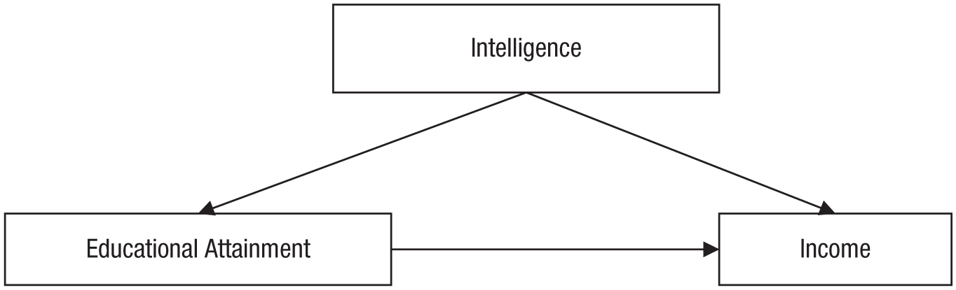
A simple directed acyclic graph depicting a causal model in which intelligence has a causal effect on both educational attainment and income, and educational attainment also has an effect on income.

One popular way to think about DAGs is to interpret them as nonparametric SEMs (Elwert, 2013), a comparison that highlights a central difference between DAGs and SEMs. Whereas SEMs encode assumptions regarding the form of the relationship between the variables (i.e., by default, arrows in SEMs indicate linear, additive relationships, unless indicated otherwise), an arrow in a DAG might reflect a relationship following any functional form (e.g., polynomial, exponential, sinusoidal, or step function). The two arrows pointing to the income node in Figure 1 indicate that income can be expressed as an arbitrary function of intelligence and educational attainment, including interactions between these two causes. In this sense, a DAG is qualitative: A → B means only that A causally affects B in some way.

Furthermore, in contrast to SEMs, DAGs allow only for single-headed arrows, which is why they are called directed graphs. Sometimes, there might be a need to indicate that two variables are noncausally associated because of some unspecified common cause, U. A double-headed arrow could be used to indicate such an association (i.e., A ↔ B), but this would just be an abbreviation of A ← U → B, which again contains only single-headed arrows.

Paths and elementary causal structures

From these two simple building blocks—nodes and arrows—one can visualize more complex situations and trace paths from variable to variable. To make this example a bit more interesting, in Figure 2 I have extended the DAG from Figure 1 by adding a new node, school grades, which are affected by intelligence and in turn affect educational attainment.

Fig. 2.

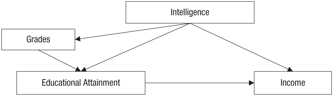
An extension of the causal model depicted in Figure 1. In this model, intelligence affects grades in school, which in turn affect educational attainment.

From this DAG, various paths can be discerned by traveling along arrows from node to node. In the simplest case, a path leads just from one node to the next one; an example is the path intelligence → income. Paths can also include multiple nodes. For example, intelligence and income are additionally connected by the paths intelligence → educational attainment → income and intelligence → grades → educational attainment → income. A path can also travel against the direction indicated by the arrows, as, for example, does the following path connecting educational attainment and income: educational attainment ← grades ← intelligence → income. Although such paths can become arbitrarily long and complex, they can be broken down into three elementary causal structures: chains, forks, and inverted forks (see also Elwert, 2013).

Chains have the structure A → B → C, for example, intelligence → educational attainment → income. Chains can transmit an association between the node at the beginning and the node at the end: If intelligence causally affects educational attainment, and educational attainment causally affects income, then intelligence and income can be correlated. Such an association reflects a genuine causal effect. In this chain, intelligence causally influences income via educational attainment.

Forks have the structure A ← B → C, for example, educational attainment ← intelligence → income. A fork can transmit an association, but it is not causal. In isolation, this fork indicates that educational attainment and income may be correlated because they share a common cause, intelligence. Forks are the causal structure most relevant for the phenomenon of confounding.

Inverted forks have the structure A → B ← C, for example, educational attainment → income ← intelligence. An inverted fork does not transmit an association: If educational attainment and intelligence both affect income, this does not imply that they are in any way correlated. Inverted forks are relevant to the problem of collider bias, which I discuss later in this article.

These three elementary causal structures determine the features of longer paths. A path that consists only of chains, such as intelligence → grades → educational attainment → income, can transmit a causal association. Along such a chain, variables that are directly or indirectly causally affected by a certain variable are called its descendants; conversely, variables that directly or indirectly affect a certain variable are considered its ancestors. For example, in this path, intelligence is an ancestor of grades, educational attainment, and income, and income is a descendant of grades.

A path that also contains forks, such as educational attainment ← grades ← intelligence → income, still transmits an association—but it is no longer a causal association because of the confounding variable (in this case, intelligence). And a path that contains an inverted fork is blocked: No association is transmitted. For example, the path educational attainment → income ← intelligence → grades does not transmit a correlation between educational attainment and grades.

No way back: acyclicity

DAGs are acyclic because they do not allow for cyclic paths in which variables become their own ancestors. A variable cannot causally affect itself; for example, in Figure 1, the direction of the path between intelligence and income cannot simply be reversed because this would result in a cyclic path (intelligence → educational attainment → income → intelligence). This may seem counterintuitive: Psychological systems often contain feedback loops, such as the reciprocal relationships in which intelligence influences education but education also influences intelligence. Such a feedback loop can be modeled in a DAG (to some extent) by taking the temporal order into account and adding nodes for repeated measures. For example, a DAG could be drawn to show that intelligence in early childhood causally influences educational attainment, which in turn influences intelligence in adulthood. Temporal resolution could be “magnified” even further and increased to annual, monthly, or even daily assessments of multiple variables, resulting in more and more nodes in the DAG. ³

Confounding: The Bane of Observational Data

With an understanding of the central terminology and rules of DAGs, we are now equipped to approach observational data in a more systematic manner. The central problem of observational data is confounding, that is, the presence of a common cause that lurks behind the potential cause of interest (the independent variable; in experimental settings, often called the treatment) and the outcome of interest (the dependent variable). Such a confounding influence can introduce what is often called a spurious correlation, which ought not to be confused with a causal effect. ⁴ How can a DAG be used to figure out how to remove all such noncausal associations so that only the true causal effect remains?

To do that, one must make sure that the DAG includes everything that is relevant to the causal effect of interest. For example, in theory, we can extend the simple DAG in Figure 2 in many different ways. Intelligence and grades are certainly not the only causes of educational attainment, and we might want to include additional variables that point to educational attainment or other nodes or add generic residuals to indicate that there are other unrelated causal influences as well as measurement error. But not all of these possible extensions of the model are of interest if we plan to investigate the causal relationship between educational attainment and income. A variable that affects educational attainment but has no causal effect on any of the other variables in the DAG—either directly or indirectly (i.e., an effect mediated by other variables)—does not need to be included. Such idiosyncratic factors, including uncorrelated measurement error, are usually not displayed, as they do not help in identifying the causal effect (Elwert, 2013). If we want to derive a valid causal conclusion, we need to build a causal DAG that is complete because it includes all common causes of all pairs of variables that are already included in the DAG (Spirtes, Glymour, & Scheines, 2000). That is, any additional variable that either directly or indirectly causally affects at least two variables already included in the DAG should be included.

After such a DAG is built, back-door paths can be discerned. Back-door paths are all paths that start with an arrow pointing to the independent variable and end with an arrow pointing to the dependent variable. In other words, back-door paths indicate that there might be a common factor affecting both the treatment and the outcome. In Figure 2, there are two such back-door paths between educational attainment and income: educational attainment ← grades ← intelligence → income and educational attainment ← intelligence → income. Back-door paths are problematic whenever they transmit an association. In this case, both back-door paths consist of only chains and forks (i.e., there are no inverted forks, which would block any transmitted association). Thus, these two back-door paths are open, and they can transmit a spurious association. The zero-order correlation between educational attainment and income is a mix of the true causal effect (educational attainment → income) of interest plus any noncausal association transmitted by the two back-door paths. To remove the undesirable noncausal association, we must block the two back-door paths.

Statistical Control: Blocking Back-Door Paths

The purpose of third-variable control is to block open back-door paths. If all back-door paths between the independent and dependent variables can be blocked, then the causal effect connecting the independent and dependent variables can be identified, even if the data are purely observational (see Pearl’s, 1993, back-door criterion). ⁵ Such a causal effect would be considered identifiable, always under the assumption that the DAG captures the true underlying causal web. Notice that the assumption that one has correctly captured the causal web and successfully blocked all back-door paths is in most cases a very strong one, because it posits that no relevant variables have been omitted from the causal graph. Whether this is plausible or not needs to be evaluated on a case-by-case basis.

A back-door path can be blocked by “cutting” the transmission of association at any point in the path by statistically controlling a node. Take, for example, the noncausal path educational attainment ← grades ← intelligence → income. We could, for example, control for grades. This would effectively block this back-door path, and it would no longer be able to transmit a noncausal association. However, we could also control for intelligence. This would again cut the transmission of this specific back-door path, but at the same time, it would also block the transmission of the second back-door path, educational attainment ← intelligence → income. If the DAG in Figure 2 correctly captured the underlying causal web, controlling for intelligence would be sufficient to identify the causal effect of educational attainment on income because it would block all back-door paths.

Various practices make it possible to control for nodes in a DAG and thus block back-door paths. Although these procedures might appear quite different from each other (i.e., they require running different statistical procedures), they serve the same purpose. In any case, if one wants to control for a certain variable, one must have measured it.

Even if the DAG correctly captures the underlying causal model, if the back-door paths that should be blocked are correctly determined, and if all the variables necessary to block all back-doors are measured, a lot can still go wrong during the actual estimation of the effect of interest. Qualitative causal identification and the subsequent quantitative (usually parametric) estimation of the identified effect are two distinct problems (Elwert, 2013): The right variables can be controlled for, but this can be done in the wrong way, as I discuss later.

How to control for a variable

Stratified analysis

In some cases, it might be possible to fully stratify the sample to control for confounders. For example, consider controlling for biological sex. Because this variable is categorical, the sample can be split into sex-homogeneous groups, analyses can be run within these groups, and the estimates from these analyses can be combined into an overall estimate. These steps would guarantee that effects of sex could not provide an alternative explanation for the findings because, for example, women have been compared only with other women. This analytic approach might be appealing because it is highly transparent. However, stratification becomes unfeasible if the third variable has many levels, if it is continuous, or if multiple third variables and their interactions need to be taken into account simultaneously. In such cases, other options for statistical control might need to be considered.

Including third variables in regression models

A widespread approach in the social sciences is to use multiple regression models to achieve statistical control. ⁶ The dependent variable can be regressed on both the independent variable and the covariate to “control for” the effects of the covariate and thus to potentially block back-door paths.

In the standard case, psychologists run models in which linear relationships are assumed without explicit justification. However, this approach does not guarantee adequate adjustment for the covariate. For example, if the effects of the covariate on the dependent and independent variables both follow a quadratic trend, linear control might leave residual confounding between the independent and dependent variables. Both the covariate and the covariate raised to the second power would need to be controlled for to properly remove the influence of the covariate in such a scenario. This point also applies to the widespread practice of “controlling for age”: Simply including age in a linear regression model will adequately adjust for age only if the age trends that need to be controlled for are approximately linear; in other cases, the statistical models might need to be refined (e.g., by including higher-order polynomials). Similarly, if covariates have interactive effects, these interactions must be considered in the model.

Matching

In many cases, there might be a need to control for not only a single third variable but for multiple ones. Furthermore, one might want to control for third variables in a fully nonparametric fashion, that is, without assuming specific functional forms for their effects. Matching is one way to approach such a situation. Different matching methods exist, but propensity-score matching is particularly popular in the social sciences. The use of propensity scores for matching is controversial, and critics have indicated that other procedures might be preferable (King & Nielsen, 2016). Nonetheless, because of the popularity of propensity-score matching, and because the fundamental rationale of matching approaches is independent of the specific method used, I focus here on the example of a study that used propensity-score matching.

Jackson, Thoemmes, Jonkmann, Lüdtke, and Trautwein (2012) were interested in the effects of military training (in comparison with civilian community service) on personality. Young men who choose to enter the military are most likely different from their civilian peers with respect to personality even before they enter the military and also differ from their civilian peers on a number of other background variables. Including all of these variables in a regression model could lead to estimation issues and result in an unwieldy model. Furthermore, such an approach would not provide an actual model of who chooses military training, which might be of interest in itself. Therefore, in their study, Jackson et al. used propensity-score matching.

First, they analyzed the covariates as predictors of the probability of entering the military. For each individual, they obtained a single number, a propensity score, that indicated how “typical” that person was of somebody joining the military. There were some individuals with high propensity scores who did not join the military, as well as some individuals with very low propensity scores who joined the military nonetheless. Subsequently, matched groups were created: For every individual with a certain propensity score who joined the military, one individual with the same (or a similar) propensity score who instead chose civilian community service was included in a control group. Under idealized conditions, this procedure would guarantee that the two resulting groups (i.e., military vs. civilian service) were balanced with respect to all control variables that were used to generate the propensity scores. Thus, these variables could no longer be the cause of any differences between the two groups being compared, and a large number of potentially confounding back-door paths would be blocked.

Such matching procedures serve the same purpose as the more common approach of including control variables. Whereas propensity scores might, depending on the circumstances, have certain advantages for estimating an effect, they do not change anything about the specifics of causal identification: If an important confounder is omitted, or if variables that should not be included are included (Sjölander, 2009), propensity scores fail to properly identify the causal effect, just as other methods of statistical adjustment do. In addition, one must again consider whether the model properly captures the effects of the covariates (e.g., whether the model underlying the propensity scores properly captures the relationships between background characteristics and the propensity to join the military).

Measurement error in confounding variables

Measurement error can affect all methods of statistical control. For example, intelligence—the confounding variable in Figures 1 and 2—cannot be measured perfectly. Thus, the statistical adjustment for intelligence is likely not able to completely remove its confounding influence, and the effect of educational attainment on income might be mistakenly assumed to be stronger than it actually is, as a result of residual confounding. The same problem holds for propensity-score matching if the scores have been based on variables that are affected by measurement error.

Westfall and Yarkoni (2016) assessed how the false positive rate for an effect is affected by measurement error of covariates that are being controlled for. It is worrisome that the false positive rate can reach very high levels, approaching almost 100%. In a worst-case scenario, applied to our example, we would almost always conclude that there is a significant effect of educational attainment on income after intelligence is controlled for, even if the association between educational attainment and income could actually be completely attributed to the confounder, intelligence. Somewhat counterintuitively, the false positive rate increases when sample sizes are large. A latent-variable approach in which the measurement error is explicitly represented in an SEM can be used to address this problem and reduce the rate of false positives; however, under realistic conditions, hundreds to thousands of participants might be required to achieve an acceptable level of statistical power (see Westfall & Yarkoni, 2016, for details).

Genetic Confounding and Control by Design

One source of potentially spurious associations that has perhaps been underappreciated in psychology is genetic confounding (e.g., between parents and their offspring). Assume that children who were rarely held and cuddled by their mothers are observed to be depressed as adults. ⁷ Before one can conclude that being raised by a cold, distant mother causes depression, it is important to consider potential back-door paths (see the DAG in Fig. 3). Mothers who are cold and distant might be so because of a certain genetic predisposition to depressiveness. A child is genetically similar to his or her mother and, thus, might inherit this predisposition, which could result in depression later in life.

Fig. 3.

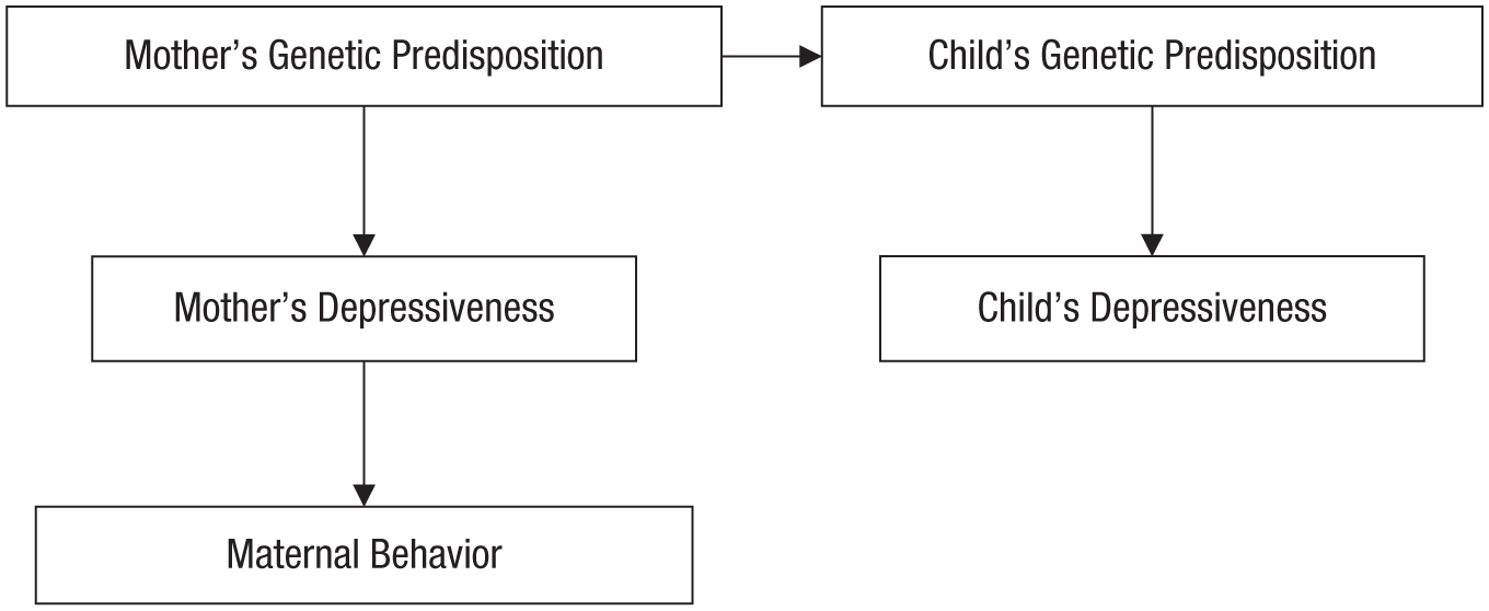
A directed acyclic graph depicting a causal model in which the link between being raised by a cold, distant mother and having depression later in life has a genetic explanation. According to this model, mothers who are genetically prone to depression may pass this genetic vulnerability on to their children, who in turn may experience similar problems later in life. In addition, mothers’ genetic predisposition to depression may result in cold, distant caregiving. In this model, there is no causal effect of mothers’ behavior on their children’s later depressiveness; any observed association between these variables is attributed to genetic confounding.

The knowledge that all traits are to some extent heritable has consequences for the ability to draw causal inferences. As Turkheimer (2000) noted, “It is no longer possible to interpret correlations among biologically related family members as prima facie evidence for sociocultural causal mechanisms” (p. 162). To figure out whether mothers’ displays of affection causally influence their children’s later depressiveness, one must block the back-door path connecting mothers’ behavior to their children’s depressiveness via genetic predispositions.

The genetic back-door path could be blocked in different ways. For example, assuming that Figure 3 depicts the correct causal model, measuring and controlling for mothers’ depressiveness would remove any spurious association.

However, in this case, an alternative to statistical adjustment is available: control by design. For example, the path between maternal and offspring genes could be blocked by sampling only adopted children, in which case there would be no link between the genetic dispositions of mothers and their offspring. ⁸ Another potentially powerful solution makes use of individuals who are matched on a wide range of variables: twins.

Monozygotic twins are of special interest for causal inference, even if a researcher is not interested in genetics at all. They are matched with respect to both their genetic predispositions and a wide range of shared family-background characteristics. Thus, they provide an attractive way to test causal claims. If a certain association is found within monozygotic twin pairs, it cannot be attributed to confounding by genes or shared family background because all these covariates have been controlled for by the design.

For example, Turkheimer and Harden (2014) investigated whether religiosity has a causal effect on delinquency and found a negative correlation when they simply correlated the variables across their whole sample. Although a causal effect might seem plausible—many religions try to encourage ethical behavior and are embedded in supportive social communities—confounders such as family-background characteristics could provide an alternative explanation. Turkheimer and Harden thus analyzed the association between religiosity and delinquency within monozygotic pairs of twins and found that the association disappeared: The more religious twin was not more (or less) likely to become delinquent than his or her twin. This finding challenges the interpretation that there might be a causal effect. If religiosity actually affected delinquency, there should have been an association even after family background and genes were controlled for.

Other “lucky accidents” and specific situations can also enable research designs that control for a wide range of potential confounders. Under ideal conditions, such designs can render additional post hoc statistical control unnecessary. These natural experiments constitute an interesting intermediate case between ordinary observational studies and randomized experiments. Such design-based approaches to causal inference are popular in economics because they often require substantially fewer assumptions than approaches that rely exclusively on third-variable control. Angrist and Pischke (2010) even suggested that design-based approaches to causal inference have spurred a “credibility revolution” in empirical microeconomics. Dunning’s (2012) excellent introduction to natural experiments (including, e.g., regression-discontinuity designs and use of instrumental variables) extensively discusses potential trade-offs in comparison with other research designs.

Learning to Let Go: When Statistical Control Hurts

In certain fields, it has become common practice to include as many covariates as possible—to the point where authors imply or claim that they have additional confidence in their findings because, for example, their study “uses more control variables than previous studies” did (Tiefenbach & Kohlbacher, 2015, p. 85). In many cases, a failure to control for important confounders will indeed undermine the conclusions, but it is not true that simply adding more covariates will always improve the estimate of a causal effect. There are two types of variables that researchers should not control for without taking into account potential negative side effects: colliders and mediators. Whereas confounders causally affect the independent variable of interest, colliders and mediators are causally affected by the independent variable. Hence, they are also referred to as posttreatment variables. A solid rule of thumb is that researchers should not control for such posttreatment variables (Rosenbaum, 1984; Rubin, 1974). In this section, I explain why.

Conditioning on a collider can introduce spurious associations

A collider for a certain pair of variables is any variable that is causally influenced by both of them. Controlling for, or conditioning analysis on, such a variable (or any of its descendants) can introduce a spurious (i.e., noncausal) association between its causes. In DAG terminology, a collider is the variable in the middle of an inverted fork, for example, variable B in A → B ← C. The collider variable normally blocks the path, but when one controls for it, a spurious association between A and C can arise. This might open up a noncausal path between the independent variable and the dependent variable of interest. In recent years, this potential source of bias has been pointed out in a variety of research fields, such as epidemiology (Greenland, 2003), personality psychology (Lee, 2012), and genetics (Munafò, Tilling, Taylor, Evans, & Smith, 2017).

Imagine that we are interested in whether the methodological rigor of a scientific study affects its innovativeness. Such an association could go either way: Methodological rigor might “tie” the hands of researchers, leading to less original research designs; but methodological rigor might also require researchers to come up with creative solutions for addressing methodological problems. For this thought experiment, let us assume that there is actually no causal effect of methodological rigor on innovativeness.

To investigate the association between methodological rigor and innovativeness, we consider all psychological studies that have been published. Say we notice that among these studies, there is a sizable negative association: Studies higher in methodological rigor are less innovative and vice versa. Next, we realize that publication bias might be an issue, so we decide to conduct a follow-up study on all psychological studies that have not been published. ⁹ In this follow-up study, we again find a sizable negative association.

By assessing published and unpublished studies separately, we have stratified our analyses by publication status; in other words, we have conditioned our analyses on publication. However, both methodological rigor and innovativeness are likely to causally affect publication status. In the simplest case, both have a positive effect: With increasing rigor, the likelihood of publication increases; with increasing innovativeness, the likelihood of publication increases. Thus, publication status is a collider (see Fig. 4). Controlling for this collider variable biases the estimate of the effect of methodological rigor on innovativeness and, in this thought experiment, introduces a negative association where no causal effect exists.

Fig. 4.

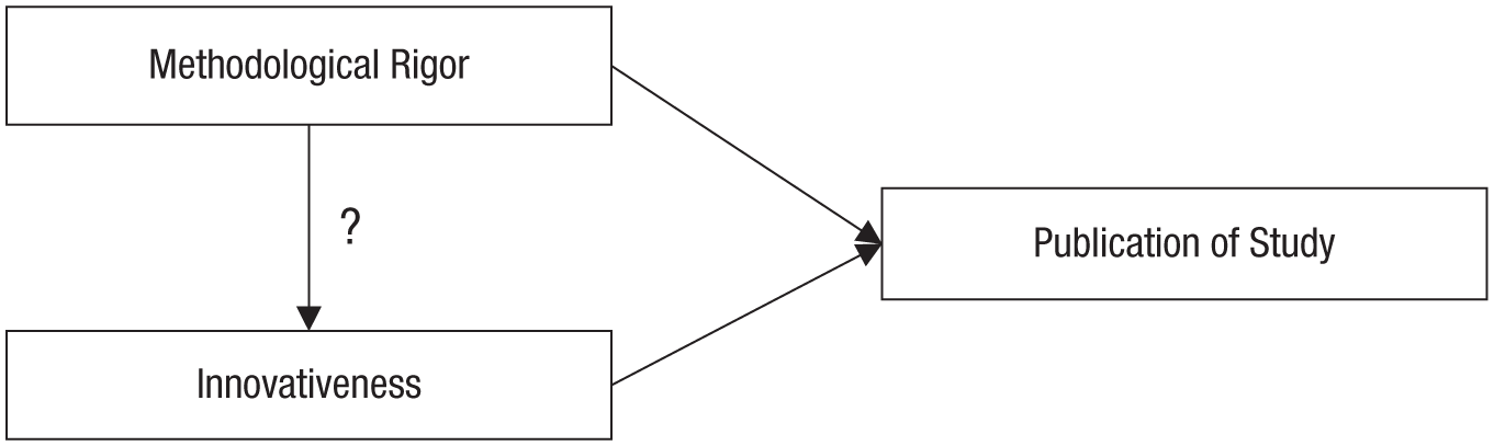
A directed acyclic graph depicting the causal model in the thought experiment on the effect of methodological rigor on the innovativeness of research. According to this model, both methodological rigor and innovativeness affect whether a study will be published or not. Thus, publication status is a collider variable, and controlling for it (e.g., by looking only at published studies) can potentially bias the estimate of the relationship between methodological rigor and innovativeness.

Collider bias seems less intuitive than spurious associations caused by confounders. However, consider what the body of published studies looks like: There are studies that are both rigorous and innovative, but such studies are likely rare if the two characteristics are uncorrelated. There are also studies that met the publication threshold thanks to high methodological rigor (despite low innovativeness) and studies that met the publication threshold thanks to high innovativeness (despite low rigor). Studies that are low in both rigor and innovativeness do not end up in this analysis, as they simply never got published. Thus, looking at all published studies (i.e., conditioning the analysis on publication) results in a negative correlation between innovativeness and rigor, giving the impression of a trade-off: Studies tend to be either rigorous or innovative. Similarly, among the unpublished studies, we observe some studies that are low on both dimensions (but such studies are rare if the characteristics are uncorrelated) as well as studies that are low on only one of the dimensions, but there are not many studies that are high on both dimensions because these ended up getting published more frequently. Again, this results in a negative association between methodological rigor and innovativeness, conditional on nonpublication.

However, in this thought experiment, there is no association between methodological rigor and innovativeness if all studies—published and unpublished—are considered simultaneously without statistical control for publication status. The spurious negative correlation emerges only when the joint outcome of the two variables of interest is controlled for. This observation generalizes to similar situations in which selection into a group is based on multiple desirable features: Group membership is a collider variable, and conditioning analysis on it will introduce or exaggerate trade-offs between desirable features. For example, people might notice that there is a negative correlation between attractiveness and intelligence among their former romantic partners. However, dating somebody is a collider of multiple causes of attraction, and, thus, it would be invalid to conclude that all potential romantic partners are either attractive or intelligent. The partner-selection procedure could have introduced a spurious correlation, because a person is relatively unlikely to date somebody who is low on both dimensions (because of lack of interest) and also relatively unlikely to end up dating somebody who is high on both dimensions (because such people are simply rare). Thus, the spurious correlation gives the impression of a trade-off (dating partners are either attractive or intelligent, but not both).

To return to the thought experiment displayed in Figure 4, the solution to the collider problem seems straightforward. If we realize that publication is a collider, we can decide to run the analysis without controlling for this variable. By extension, we should also not control for descendants of the collider variable. For example, the publication of a study might have a causal effect on whether or not popular media report about the findings. If we look only at studies that have been covered by popular media—that is, if we condition our analysis on this descendant of the collider—we might observe the same spurious negative association between methodological rigor and innovativeness.

Avoiding collider bias requires two steps. First, one must be aware of the collider variable, and second, one must be able to run analyses that are not conditional on the collider (e.g., in our thought experiment, we must include both published and unpublished studies). Outside of thought experiments, one might often be unaware of collider variables or collect data in such a way that collider bias is built in.

Variations on the theme of collider bias

Collider bias that results from the sampling procedure (and not from, e.g., the inclusion of inadequate covariates) has also been labeled endogenous selection bias. Elwert and Winship (2014) provided a succinct summary of the many ways in which endogenous selection bias can arise. In the following, I briefly illustrate this form of collider bias with examples that might be relevant to psychologists.

Nonresponse bias

Nonresponse bias occurs if, for example, a researcher analyzes only completed questionnaires, and the variables of interest are associated with questionnaire completion. Assume that we are interested in the association between grit and intelligence, and our assessment ends up being very burdensome. Both grit and intelligence make it easier for respondents to push through and complete the assessment. Questionnaire completion is thus a collider between grit and intelligence. For example, although there might be no association between grit and intelligence in the population, we might find a spurious negative association if we analyze only completed questionnaires. That is, completers low on intelligence may have compensated with their high levels of grit, completers low on grit may have compensated with their high levels of intelligence, and invited participants who were low on both variables may have been less likely to finish the assessment and thus be underrepresented in the analyzed sample.

Attrition bias

Assume that we are conducting a longitudinal study and are interested in the effects of health problems on work satisfaction. We assessed work satisfaction at a later point in time, which supposedly gives us confidence in the direction of the causal flow. However, over time, respondents inevitably dropped out of the study (e.g., they moved away, could not be found, were no longer willing to participate), and this attrition was likely selective. Some respondents might have left the study because of health problems; others might have dropped out because their workplace was too stressful (see Fig. 5 for a DAG depicting this scenario). Now, assume that we analyze data from only those respondents who remained in our sample.

Fig. 5.

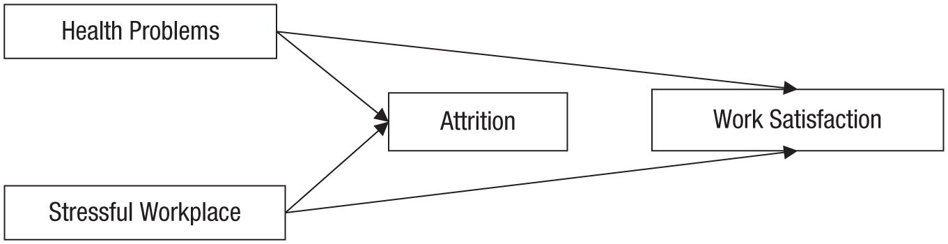
A directed acyclic graph depicting the causal model of the thought experiment on the effect of health problems on work satisfaction. In this model, attrition is causally affected by both health problems and having a stressful workplace. If analyses include only the respondents who remained in the sample, they are conditioned on a collider that potentially induces a spurious association between health problems and a stressful workplace. This association opens a back-door path that potentially introduces a noncausal association between health problems and work satisfaction.

If only the respondents remaining in the panel are included in the analysis, spurious associations between all causes of attrition can arise, and they might open up a back-door path between the variables of interest. In this example, attrition could introduce a spurious association between health problems and a stressful workplace. Both health problems and a stressful workplace likely led to attrition; respondents with health problems might have remained in the study if they had low-stress jobs, and respondents with a stressful workplace might have remained in the study if they were in particularly robust health. Assuming that there is a negative effect of health problems on work satisfaction, the strength of this association would be underestimated if only the final sample is analyzed because the respondents with greater health problems were more likely to work in low-stress workplaces, which are generally more likely to leave individuals satisfied.

Related issues: missingness and representativity

Thoughts about endogenous selection bias quite naturally lead to consideration of certain problems that normally are not framed as concerns for causal inference. One such problem is missing data. Nonresponse and attrition bias lead to missing data, and these missing data must be handled properly if the goal is to draw valid causal conclusions on the basis of observational data. Schafer and Graham (2002) have provided an introduction to the management of missing data for psychologists. Thoemmes and Mohan (2015) used DAGs based on formalizations by Mohan, Pearl, and Tian (2013) to provide visual representations of missing-data scenarios.

Another problem related to endogenous selection bias is nonrepresentativeness of samples (i.e., samples that do not accurately reflect the underlying population about which the researchers want to make statements). For example, if a researcher investigates only college students, endogenous selection bias is introduced between all variables that causally affect whether or not somebody becomes a college student (e.g., socioeconomic status, cognitive abilities, attitudes, parents’ characteristics).

Controlling for mediators: removing the association of interest

Overcontrol bias is another example of statistical control hurting instead of helping: If mediating variables are controlled for, the very processes of interest are controlled away. This point can be illustrated by returning to the example in Figure 1 and additionally assuming that educational attainment has an influence on intelligence in adulthood. Although this might still seem like a grossly oversimplified model of reality, it results in considerably more complex considerations. In addition, let us incorporate a variable labeled U (see Fig. 6). Although it is possible to come up with plausible ideas about what U stands for (i.e., some variable that affects both adult intelligence and income, potentially something unobserved), let us simply leave it unspecified here, as conceptual considerations derived from a DAG do not depend on the concrete variables but depend only on the underlying abstract causal web.

Fig. 6.

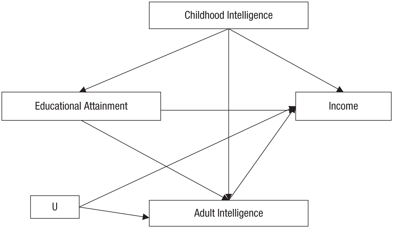
A directed acyclic graph extending the causal model in Figure 1 by adding intelligence in adulthood and an unknown variable labeled U. In this model, intelligence in childhood confounds the association between educational attainment and income, but at the same time, intelligence in adulthood is a mediator of the effect of educational attainment on income. In addition, intelligence in adulthood and income are confounded by U.

Again, childhood intelligence is a confounder that needs to be controlled for. However, the question is whether we should or should not control for intelligence in adulthood. Adult intelligence is a mediator of the effects of educational attainment on income; it is a node on a causal pathway between those variables. If we were able to randomly assign participants to different educational paths, this manipulation would also affect their intelligence, which in turn would affect their income. Controlling for adult intelligence would block this genuinely causal pathway, and we would likely underestimate the positive payoff of getting a college education. If one is interested in the magnitude of a causal effect, one should not control for mediating variables (i.e., the mechanisms driving the effect). By extension, one should not control for any descendant of a mediating variable. Consider, for example, what we should do if we add chess performance in adulthood as an outcome of adult intelligence in our model. Chess performance is a noisy proxy for intelligence, and controlling for it will remove some of the variation in adult intelligence that is caused by the independent variable of interest (i.e., educational attainment). Thus, we should not control for this descendant of the mediating mechanism.

In some cases, researchers might actually be interested in the effect of an independent variable on a dependent variable after accounting for the effect of a mediating variable. This is a common goal of mediation analysis. Both old and newer common approaches to estimating the remaining (direct) effect after accounting for a mediator (e.g., Baron & Kenny, 1986; Hayes, 2009) rely on statistical control of the mediating variable, but such approaches can introduce endogenous selection bias (Elwert & Winship, 2014).

In Figure 6, adult intelligence is a collider with respect to educational attainment and U. As long as adult intelligence is not controlled for, U is unproblematic: It affects the outcome variable (i.e., income), but it does not causally affect the independent variable (i.e., educational attainment); thus, U is not a confounder of the effect of interest and can simply be ignored. However, if adult intelligence is controlled for, a noncausal association between its two causes, U and educational attainment, is introduced (i.e., educational attainment ↔ U). Now, a back-door path, educational attainment ↔ U → income, has been opened, and it potentially introduces a noncausal association. If the goal is to correctly estimate the direct effect of a college degree on income, all back-door paths opened by conditioning the analysis on the mediating variable must be blocked.

Maybe somewhat surprisingly, this problem of mediation analysis also applies to experimental studies unless the mediating variable itself was randomly assigned. Randomized assignment of the independent variable rules out back-door paths between the independent variable and dependent variable, but back-door paths between the mediator and the dependent variable remain unaffected. In such a study, estimating the direct effect by controlling for the mediating variable can lead to biased estimates. In offering recommendations for experimental research programs, Bullock, Green, and Ha (2010) highlighted that uncovering a mediating mechanism might be much harder than most social scientists realize.

Conclusion: Making Causal Inferences on the Basis of Correlational Data Is Very Hard

To summarize, the practice of making causal inferences on the basis of observational data depends crucially on awareness of potential confounders and meaningful statistical control (or noncontrol) that takes into account estimation issues such as nonlinear confounding and measurement error. Back-door paths must be considered before data are collected to make sure that all relevant variables are measured. In addition, variables that should not be controlled for (i.e., colliders and mediators) need to be considered. This might require careful planning before data collection begins because researchers must consider how sample recruitment might result in endogenous selection bias, which threatens the validity of any conclusions drawn.

In reality, researchers may often end up with data that do not contain reliable measures of central confounders—because a back-door path was not considered before the data were collected (or before comments were made by peer reviewers), because somebody else collected the data (e.g., they came from nationally representative panel or survey studies), or because the confounder is some unobservable factor that could not be measured with available methods. In such a situation, thorough consideration of the causal web underlying the variables can lead to the conclusion that the data do not warrant causal claims.

In addition, in a messy psychological reality, causal graphs quickly become substantially more complex than the illustrations included in this article. For example, in certain constellations of variables, controlling for a variable might reduce one type of bias (because the variable is a confounder) but at the same time increase another type of bias (because the variable is a collider on a different path that transmits a spurious association when the collider is controlled for). Such a constellation, which produces what is called butterfly bias, can be easily visualized in a DAG. Quite pragmatically, one can gauge which of the two biases is more problematic and then settle for the lesser evil (Ding & Miratrix, 2015).

In other cases, it can be genuinely unclear whether a given variable is a confounder, collider, or mediator. Strong theories that posit clear directional links between variables might solve such problems, but in some cases, theory might simply indicate that different data are needed. For example, if educational attainment, intelligence, and income are measured at only one point in time, it is unclear whether intelligence should be controlled for or not—the variable certainly captures confounding influences, but at the same time, it also capture parts of the “treatment” of education. Reciprocal effects seem plausible for many psychological variables, and to disentangle causes and effects in such a situation, one needs data with a higher temporal resolution than results from typical psychological designs, which often consist of only a few measurement waves. Again, thoughtful consideration of the underlying causal web might lead to the conclusion that the data at hand are not sufficient and that different sampling designs, such as intensive time series of repeated measures (Borsboom et al., 2012), are needed.

Causal inferences based on observational data require researchers to make very strong assumptions. Researchers who attempt to answer a causal research question with observational data should not only be aware that such an endeavor is challenging, but also understand the assumptions implied by their models and communicate them transparently. In addition, instead of reporting a single model and championing it as “the truth,” researchers should consider multiple potentially plausible sets of assumptions and see how assuming any of these scenarios would affect their conclusions. This practice of robustness checking is already common in some subfields of economics and could also improve inference in psychological research (see, e.g., Duncan, Engel, Claessens, & Dowsett, 2014, for recommendations for developmental research). As a positive side effect, performing and reporting multiple analyses (i.e. conducting a “multiverse analysis”; Steegen, Tuerlinckx, Gelman, & Vanpaemel, 2016) can greatly improve transparency and thus facilitate productive and open debates.

One could argue that—given the complex nature of human behavior—causal modeling of observational data might not be worth the hassle, as it requires a great deal of effort with respect to both theoretical reasoning and data collection and nonetheless results in claims that can often be easily challenged. However, this should not be a reason to give up the endeavor altogether.

Although properly implemented randomized experiments leave researchers with great confidence in internal validity, “their meaning and significance for the target phenomenon are often questionable” (Rozin, 2001, p. 12). That is, randomized experiments allow researchers to be confident about a cause-effect relationship with only very few additional assumptions, but many more assumptions might be needed to convincingly argue that this cause-effect relationship is actually the one of interest. Which method—randomized experiment, natural experiment, or observational study—is suited for drawing a causal inference regarding a specific research question must be decided on a case-by-case basis (see also Cartwright’s, 2007, arguments that there is no gold standard).

It is instructive to consider cases in which most people readily accept causal claims in the absence of randomized experiments. Nowadays, few people doubt the effects of tobacco smoking on lung cancer. But in the 1950s, tobacco lobbyists embraced the idea that a genetic predisposition caused both a tendency to smoke and lung cancer (Mukherjee, 2010, p. 253). In other words, they claimed that there was an unblocked back-door path. This idea was dispelled not by randomized, controlled experiments in humans, but by highly consistent results of observational studies using various controls and different sampling designs, experimental evidence from rodent studies, and demonstration of a plausible mechanism (i.e., inhaled carcinogens correlate with visible malignant changes in the lung, which in turn correlate with lung cancer; see Mukherjee, 2010, for a summary of the history of cancer research).

A plausible mechanism is also what greatly increases scientists’ confidence in the causal effect of human activity on the climate: Human activity, such as industrial processes, increases the atmospheric concentrations of greenhouse gases. Atmospheric greenhouse gases, in turn, warm the Earth’s surface through an uncontroversial mechanism, the greenhouse effect (see Silver, 2012, p. 374, for this line of argument). And a plausible mechanism is also the reason why one does not need randomized controlled trials to conclude that parachute use during free fall reduces mortality (but cf. Smith & Pell, 2003).

Thus, causal inference based on observational data is not a lost cause per se—indeed, in combination with additional knowledge from the relevant domain, highly convincing causal arguments can be made. Further research into psychological mechanisms and processes, which will frequently involve experimental studies, including well-designed surrogate interventions, can strengthen the potential of observational data. Likewise, observational data can be used to ensure the external validity of findings from constrained experimental settings and also hint toward new phenomena that potentially warrant further research. Different research designs are neither mutually interchangeable nor rivals, but can contribute unique information to help answer common research questions. The most convincing causal conclusions will always be supported by multiple designs. As Angrist and Pischke (2010) noted, “In the empirical universe, evidence accumulates across settings and study designs, ultimately producing some kind of consensus” (p. 25).