
Abstract
This Tutorial serves as both an approachable theoretical introduction to mixed-effects modeling and a practical introduction to how to implement mixed-effects models in R. The intended audience is researchers who have some basic statistical knowledge, but little or no experience implementing mixed-effects models in R using their own data. In an attempt to increase the accessibility of this Tutorial, I deliberately avoid using mathematical terminology beyond what a student would learn in a standard graduate-level statistics course, but I reference articles and textbooks that provide more detail for interested readers. This Tutorial includes snippets of R code throughout; the data and R script used to build the models described in the text are available via OSF at https://osf.io/v6qag/, so readers can follow along if they wish. The goal of this practical introduction is to provide researchers with the tools they need to begin implementing mixed-effects models in their own research.
In many areas of experimental psychology, researchers collect data from participants responding to multiple trials. This type of data has traditionally been analyzed using repeated measures analyses of variance (ANOVAs)—statistical analyses that assess whether conditions differ significantly in their means, accounting for the fact that observations within individuals are correlated. Repeated measures ANOVAs have been favored for analyzing this type of data because using other statistical techniques, such as multiple regression, would violate a crucial assumption of many statistical tests: the independence assumption. This assumption states that the observations in a data set must be independent; that is, they cannot be correlated with one another. But take, for example, a reaction time study in which participants respond to the same 100 trials, each of which corresponds to a different item (e.g., a particular word in a psycholinguistics study). Reaction times within a given participant and within an item will certainly be correlated; some participants are faster than others, and some items are responded to more quickly than others. Given that observations are not independent, data in which participants respond to multiple trials must be analyzed with a statistical test that takes the dependencies in the data into account.
For this reason, when analyzing data in which observations are nested within participants, repeated measures ANOVAs are preferable to standard ANOVAs and multiple regression, which both ignore the hierarchical structure of the data. However, repeated measures ANOVAs are far from perfect. Although they can model either participant- or item-level variability (often referred to as F1 and F2 analyses in the ANOVA literature), they cannot simultaneously take both sources of variability into account, so observations within a condition must be collapsed across either items or participants. When the data are aggregated in this way, however, important information about variability within participants or items is lost, which reduces statistical power (see Barr, 2008), that is, the likelihood of detecting an effect if one exists.
Another limitation of ANOVAs is that they deal with missing observations via listwise deletion; this means that if a single observation is missing, the entire case is deleted, and none of the observations from that individual (or item) will be used in the analysis. Depending on the number of complete cases in the data set, this can substantially reduce sample size, which leads to inflated standard error estimates and reduced statistical power (though the estimates will be unbiased if the data are missing completely at random; see Enders, 2010). ANOVAs also assume that the dependent variable is continuous and the independent variables are categorical; experiments in which the outcome is categorical (e.g., accuracy at identifying particular items in a recognition memory task) must be aggregated or analyzed using a different technique, and continuous predictors (e.g., time in a longitudinal study) must be treated categorically (i.e., binned), which reduces statistical power and makes it difficult to model nonlinear relationships between predictors and outcomes (e.g., Liben-Nowell et al., 2019; Royston et al., 2005). A final drawback of ANOVAs is that although they indicate whether an effect is significant, they do not provide information about the magnitude or direction of the effect; that is, they do not provide individual coefficient estimates for each predictor that indicate growth or trajectory.
Mixed-Effects Models Take the Stage
These shortcomings of ANOVAs and multiple regression can be avoided by using linear mixed-effects modeling (also referred to as multilevel modeling or mixed modeling). Mixed-effects modeling allows a researcher to examine the condition of interest while also taking into account variability within and across participants and items simultaneously. It also handles missing data and unbalanced designs quite well; although observations are removed when a value is missing, each observation represents just one of many responses within an individual, so removal of a single observation has a much smaller effect in the mixed-modeling framework than in the ANOVA framework, in which all responses within a participant are considered to be part of the same observation. Participants or items with more missing cases also have weaker influences on parameter estimates (i.e., the parameter estimates are precision weighted), and extreme values are “shrunk” toward the mean (for more details on shrinkage, see Raudenbush & Bryk, 2002; Snijders & Bosker, 2012). Further, continuous predictors do not pose a problem for mixed-effects models (see Baayen, 2010), and the fitted model provides coefficient estimates that indicate the magnitude and direction of the effects of interest. Finally, the mixed-effects regression framework can easily be extended to handle a variety of response variables (e.g., categorical outcomes) via generalized linear mixed-effects models, and operating in this framework makes the transition to Bayesian modeling easier, as reliance on ANOVAs tends to create a fixed mind-set in which statistical testing and categorical “significant versus nonsignificant” thinking are paramount. Mixed-effects modeling is therefore appropriate in many cases in which standard ANOVAs, repeated measures ANOVAs, and multiple regression are not. Thus, it is a more flexible analytic tool.
Disclosures
The data and R script used to generate the models described in this article are available via OSF, at https://osf.io/v6qag/.
Introducing the Data
In this Tutorial, I use examples from my own research area, human speech perception, but the concepts apply to a wide variety of areas within and beyond psychology. For example, participants in a social-psychology experiment might view videos and be asked to evaluate the affect associated with each of them, or participants in a clinical experiment might read a series of narratives and be asked to describe the extent to which each of them generates anxiety. 1 The goal of this Tutorial is to provide a practical introduction to linear mixed-effects modeling and introduce the tools that will enable you to conduct such analyses on your own. This overview is not intended to address every issue you may encounter in your own analyses, but is meant to provide enough information that you have a sense of what to ask if you get stuck. To help you along the way, I provide snippets of R code using dummy data that serve as a running example.
The example data I provide (see https://osf.io/v6qag/), which we will work with later in this Tutorial, come from a within-subjects speech-perception study in which each of 53 participants was presented with 553 isolated words, some in the auditory modality alone (audio-only condition) and some with an accompanying video of the talker (audiovisual condition). Participants listened to and repeated these isolated words aloud while simultaneously performing an unrelated response time task in the tactile modality (classifying the length of pulses that coincided with the presentation of each word as short, medium, or long). The response time data are based on data from a previous experiment of mine (Brown & Strand, 2019; complete data set available at https://osf.io/86zdp/), but the response times themselves have been modified for pedagogical purposes (i.e., to illustrate particular issues that you may encounter when analyzing data with mixed-effects models). The accuracy data have not been modified, but variables have been removed for simplicity.
Previous research has shown that being able to see as well as hear a talker in a noisy environment substantially improves listeners’ ability to identify speech relative to hearing the talker alone (e.g., Erber, 1972). The goals of this dual-task experiment were to determine whether seeing the talker would also affect response times in the secondary task (slower response times were taken as an indication of increased cognitive costs associated with the listening task—“listening effort”) and to replicate the well-known intelligibility benefit from seeing the talker. In what follows, we will use mixed-effects modeling to assess the effect of modality (audio-only vs. audiovisual) on response times and word intelligibility while simultaneously modeling variability both within and across participants and items. We will assume that modality was manipulated within subjects and within items, which means that each participant completed the task in both modalities, and each word was presented in both modalities (but each word occurred in only one modality for each participant).
For all the analyses described below, we will use a dummy-coding (also referred to as treatment-coding) scheme such that the audio-only condition serves as the reference level and is therefore coded as 0, and the audiovisual condition is coded as 1. Thus, in the mixed-effects models, the regression coefficient associated with the intercept represents the estimated mean response time in the audio-only condition (when modality = 0), and the coefficient associated with the effect of modality indicates how the mean response time changes in the audiovisual condition (when modality = 1). We could instead use the audiovisual condition as the reference level, in which case the intercept would represent the estimated mean response time in the audiovisual condition (when modality = 0), and the modality effect would indicate how this estimate changes in the audio-only condition (when modality = 1). Altering the coding scheme, either by changing the reference level or by switching to a different coding scheme altogether (e.g., sum or deviation coding, which involves coding the groups as −0.5 and 0.5 or −1 and 1 so the intercept corresponds to the grand mean) will not change the fit of the model; it will simply change the interpretation of the regression coefficients (but often leads to misinterpretation of interactions, as I discuss below; see Wendorf, 2004, for a description of various coding schemes).
The left side of Table 1 shows the first six lines of the data in the desired format: unaggregated long format. For a helpful tutorial on how to wrangle the data into this format, I recommend Wickham and Grolemund’s (2017) open-access textbook R For Data Science (Chapter 12.3.1) and the tidyverse collection of R packages (Wickham et al., 2019). If you are following along with your own data, ensure that your data are in long format such that each row represents an individual observation (i.e., do not aggregate across either participants or items). Notice that in this half of the table, each of the first six rows corresponds to a different word (
First Six Rows of the Example Data Set in Unaggregated and Aggregated Formats

Note:
Fixed and Random Effects
Mixed-effects models are called “mixed” because they simultaneously model fixed and random effects. Fixed effects represent population-level (i.e., average) effects that should persist across experiments. Condition effects are typically fixed effects because they are expected to operate in predictable ways across various samples of participants and items. Indeed, in our example, modality will be modeled as a fixed effect because we expect that there is an average relationship between modality and response times that will turn up again if we conduct the same experiment with a different sample of participants and items.
Whereas fixed effects model average trends, random effects model the extent to which these trends vary across levels of some grouping factor (e.g., participants or items). Random effects are clusters of dependent data points in which the component observations come from the same higher-level group (e.g., an individual participant or item) and are included in mixed-effects models to account for the fact that the behavior of particular participants or items may differ from the average trend. Given that random effects are discrete units sampled from some population, they are inherently categorical (Winter, 2019). Thus, if you are wondering if an effect should be modeled as fixed or random and it is continuous in nature, be aware that it cannot be modeled as a random effect and therefore must be considered a fixed effect. In our hypothetical experiment, participants and words are modeled as random effects because they are randomly sampled from their respective populations, and we want to account for variability within those populations.
Including random effects for participants and items resolves the nonindependence problem that often plagues multiple regression by accounting for the fact that some participants respond more quickly than others, and some items are responded to more quickly than others. These random deviations from the mean response time are called random intercepts. For example, the model may estimate that the mean response time for some condition is 1,000 ms, but specifying by-participant random intercepts allows the model to estimate each participant’s deviation from this fixed estimate of the mean response time. So if one participant tended to respond particularly quickly, that person’s individual intercept might be shifted down 150 ms (i.e., the estimated intercept would be 850 ms). Similarly, including by-item random intercepts enables the model to estimate each item’s deviation from the fixed intercept, reflecting the fact that some words tend to be responded to more quickly than others. In multiple regression, in contrast, the same regression line (both intercept and slope) is applied to all participants and items, so predictions tend to be less accurate than in mixed-effects regression, and residual error tends to be larger. Thus, in mixed modeling, the fixed-intercept estimate represents the average intercept, and random intercepts allow each participant and item to deviate from this average. 2 These deviations are assumed to follow a normal distribution with a mean of zero and a variance that is estimated by the model.
An additional source of variability that mixed-effects models can account for comes from the fact that a variable that is modeled as a fixed effect may actually have different influences on different participants (or items). In our example, some participants may show very small differences in response times between the audio-only and audiovisual conditions, and others may show large differences. Similarly, some words may be more affected by modality than others. To model this type of variability, we will include random slopes in the model specification. In our hypothetical study, the model may estimate that the effect of modality is 83 ms—meaning that participants were, on average, 83 ms slower in the audiovisual condition than the audio-only condition—but one participant may have been very strongly affected by modality (e.g., a response time difference between modalities of 200 ms), and another may have been only weakly affected by modality (e.g., a response time difference between modalities of 10 ms). These individual deviations from the average modality effect are modeled via random slopes (note that a simple mean difference like the one described here is represented in a regression equation as a slope).
It may be confusing that modality comes up in the context of fixed and random effects, but recall that an effect is considered fixed if it is assumed that the effect would persist in a different sample of participants. In our case, modality is modeled as a fixed effect because we are modeling the common influence of modality on response times across participants and items. However, given that participants represent a random sample from the population of interest, the effect of modality within participants represents a subset of possible ways modality and participants can interact. In other words, modality itself is not a random effect, but the way it interacts with participants is random, and including random slopes for modality allows the model to estimate each participant’s deviation from the overall (fixed) trend. (For more on the distinction between fixed and random effects and a description of when a researcher may actually want to model participants as a fixed effect, see Mirman, 2014).
One question people often have at this point is, if mixed-effects models derive an intercept and slope estimate for each participant, why are these seemingly systematic effects called random effects? The answer is that although an effect might be consistent within a particular individual (e.g., one participant may systematically respond more quickly and be less affected by modality than average), the source of this variability is unknown and is therefore considered random. If you find yourself stumbling over the use of the word random, it may be helpful to instead consider the synonymous terminology by-participant (or -item) varying intercepts (or slopes). However, given that these effects are most commonly referred to as random intercepts and slopes, I use that terminology here.
Visualizing Random Intercepts and Slopes
In this section, I provide plots to help you visualize what happens when one builds on ordinary regression by introducing random intercepts and random slopes. These plots are derived from fake data from four hypothetical participants who each responded to four items (note that random effects really should have at least five or six levels, and having more levels is preferable; e.g., Bolker, 2020). The effect of interest is the influence of word difficulty on response times (where 0 represents “very easy” by some collection of criteria, such as the frequency with which the word occurs in the language and the number of similar-sounding words, and 10 represents “very difficult”). First, consider a model with no random effects (i.e., fixed-effects-only regression; Fig. 1). More difficult words tend to elicit slower response times, but because there are no random effects, the model estimates are the same for every participant; that is, although you can tell which points in the plot correspond to each participant because I have represented data from each participant with a different shape, the model does not have access to this information. Further, given that this model predicts just one regression line that applies to all observations, the residual error (represented by vertical lines connecting every point to the regression line) is relatively large.

Fixed-effects-only regression line depicting the relationship between word difficulty and response time. The plotted points represent individual response times for each word for each participant, and the vertical lines represent the deviation of each point from the line of best fit (i.e., residual error). Note that although you can discern the nested nature of the data from this plot because each participant’s data are represented by a different shape, the model does not take such dependencies in the data into account. For visualization purposes, data from the four participants for each word have been jittered horizontally to avoid overlap.
Next, consider a model that includes random intercepts for participants. In Figure 2, each dashed gray line depicts model predictions for a single participant, and the solid black line depicts the estimates for the average (fixed) effects. This model takes into account the fact that some participants tend to have slower response times than others. Here, the overall effect of word difficulty on response times is still apparent, but this model does a better job predicting response times for a given participant because it allows for each participant to have a different intercept (representing the predicted response time for a word with a 0 on the difficulty scale). In this example, the relationship between word difficulty and response time is equally strong for all participants (i.e., the slope is fixed); random intercepts simply shift each participant’s regression line up or down depending on that individual’s deviation from the mean (see Winter, 2019, p. 237, for another way of visualizing random intercepts, via a histogram of each individual’s deviation from the population intercept). Notice that the residual error, indicated by the vertical lines, is substantially smaller in the random-intercepts model relative to the fixed-effects-only model. Indeed, the residual standard deviation in the original model is 410 ms, but it is reduced to 275 ms in the random-intercepts model (these values are obtained via the

Mixed-effects regression lines depicting the relationship between word difficulty and response time, generated from a model including by-participant random intercepts but no random slopes. Each dashed gray line represents model predictions for a single participant, and the solid black line represents the fixed-effects estimates for the intercept and slope. The plotted points represent individual response times for each word for each participant, and the vertical lines represent the deviation of each point from the participant’s individual regression line. Notice that including random intercepts reduces residual error relative to the error in the fixed-effects-only model (Fig. 1). For visualization purposes, data from the four participants for each word have been jittered horizontally to avoid overlap.
Figure 3 shows how the model changes when by-participant random slopes are included; this model allows for the relationship between word difficulty and response time to vary across participants. Here, participants differ not only in how quickly they respond when word difficulty is 0 (random intercepts), but also in the extent to which they are affected by changes in word difficulty (random slopes). Although the general trend that difficult words are responded to more slowly is still apparent, the strength of this relationship varies across participants. The result is that the residual error is even smaller because each regression line is tailored to the individual; indeed, the residual standard deviation has decreased from 275 ms in the random-intercepts model to 75 ms in the random-slopes model. Note that for simplicity, these plots do not take item-level variability into account. (See Barr et al., 2013, for a helpful visualization depicting the simultaneous influences of participant and item random effects.)
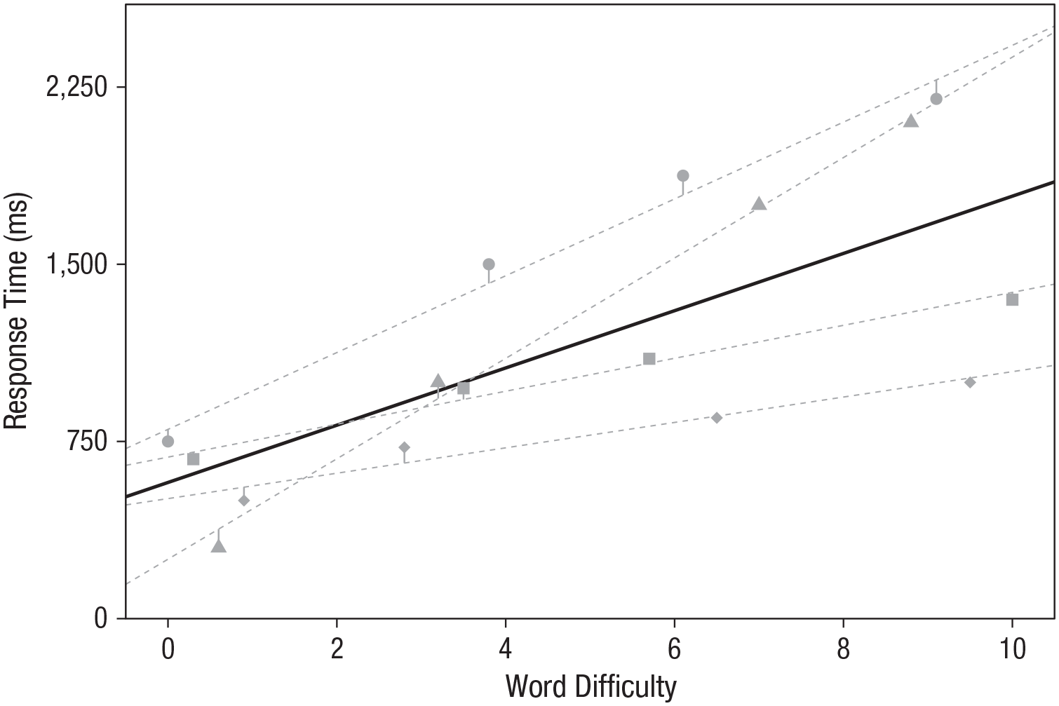
Mixed-effects regression lines depicting the relationship between word difficulty and response time, generated from a model including by-participant random intercepts as well as by-participant random slopes for word difficulty. Each dashed gray line represents model predictions for a single participant, and the solid black line represents the fixed-effects estimates for the intercept and slope. The plotted points represent individual response times for each word for each participant, and the vertical lines represent the deviation of each point from the participant’s individual regression line. Notice that including random slopes reduces residual error relative to the error in both the random-intercepts model and the fixed-effects-only model (Figs. 1 and 2). For visualization purposes, data from the four participants for each word have been jittered horizontally to avoid overlap.
Correlations Among Random Effects
The discussion of mixed-effects models thus far has focused on fixed effects, random intercepts, and random slopes, but the models estimate additional parameters that are often overlooked: correlations among random effects. For example, when you specify that a model should include by-participant random intercepts and slopes for modality, the model will also estimate the correlations among those random intercepts and slopes. Although experimental psychology typically focuses on fixed effects, correlations among random effects can provide useful information about individual differences in condition effects.
Suppose, for example, that in our hypothetical dual-task experiment, the correlation between the by-participant random intercepts and slopes was negative (e.g., r = −.17). This would suggest that individuals who have higher intercepts (i.e., slower response times in the audio-only condition) tend to have lower slopes. Interpreting what “lower” means in the context of our experiment also requires knowledge of the direction of the modality effect. If the modality effect is positive, then “lower slopes” means slopes that are less positive (i.e., closer to zero), and the correlation therefore suggests that individuals with slower response times are less affected by the modality manipulation. If, however, the modality effect is negative, then “lower slopes” means slopes that are more negative, which suggests that individuals with slower response times tend to be more affected by the condition manipulation.
If the modality effect is 83 ms, a negative correlation between by-participant random intercepts and slopes would indicate that individuals who had slower response times in the audio-only condition tended to show a less pronounced slowing in the audiovisual condition. One interpretation of this correlation is that people who respond more slowly are completing the task more carefully, and this slow, deliberate responding washes out the condition effect in those individuals. Although this correlation is not of particular interest in this experiment, there are situations in which correlations among random effects are key to the research question. For example, a researcher conducting a longitudinal study might be interested in whether students’ baseline mathematical abilities are related to the trajectory of their improvement over the course of a training program, so the correlation between by-participant random intercepts and slopes for the training effect would be of particular interest.
Another reason for examining correlations among random effects is that they can be informative about possible ceiling or floor effects. Consider the intelligibility effect I described when I introduced the data: Seeing the talker improves speech intelligibility. A negative correlation between by-participant random intercepts and slopes for modality in this case would indicate that individuals with higher intercepts (i.e., better speech identification in the audio-only condition) had shallower slopes (i.e., benefited less from seeing the talker)—a correlation that would also emerge if the speech-identification task was too easy. That is, if participants could attain a high level of performance without seeing the talker, then seeing the talker would have little effect on performance; this would result in a negative correlation between by-participant random intercepts and slopes, but only because ceiling effects prevented the modality effect from emerging in some individuals (see Winter, 2019, p. 239, for another example of random-effects correlations that may indicate the presence of ceiling effects). Thus, even if your research question primarily concerns fixed effects, examining random effects and their correlations will help you understand your data more deeply.
Which Random Effects Can You Include?
Before we move on to implementation in R, it is important to note one other issue regarding random-effects structures in mixed-effects modeling: deciding which random slopes are justified by your design. Consider again the example in which we modeled response times to words as a function of their difficulty. Word difficulty was manipulated within subjects, but because the words differed on an intrinsic property—namely, their difficulty—word difficulty was a between-items variable. Given that by-item random slopes account for variability across items in the extent to which they are affected by the predictor of interest, we cannot model the effect of word difficulty on a particular item because each word has only one level of difficulty; that is, we cannot include by-item random slopes. 3 In contrast, if the predictor of interest was a within-items variable (as in our running example in which all words appeared in both the audio-only and the audiovisual conditions), we could include by-item random slopes for that predictor in our model, which would account for the fact that different words may be differently affected by the predictor. Put simply, by-participant and by-item slopes are justified only for within-subjects and within-items designs, respectively. Thus, our random-effects structure in the word-difficulty example can include random intercepts for both participants and items, as well as by-participant random slopes for word difficulty, but cannot include by-item random slopes for word difficulty.
Because including by-item random slopes for word difficulty would not be justified in this example, the random-effects structure including random intercepts for both participants and items, as well as by-participant random slopes for word difficulty, would represent the maximal random-effects structure justified by the design (see Barr et al., 2013; Matuschek et al., 2017). In cases in which by-participant and by-item random slopes are justified, mixed-effects models can incorporate the simultaneous influences of both participant and item random slopes (but note that just because you can include a random effect does not necessarily mean that it would be advisable to do so. I discuss this further in the Model Building and Convergence Issues section).
Examples and Implementation in R
Now that you have a conceptual understanding of what mixed-effects models are and why they are useful, let us consider how to implement them in R. First, you will need to install R (R Core Team, 2020) and then RStudio (RStudio Team, 2020), a programming environment that allows you to write R code, run it, and view graphs and data frames all in one place. I suggest working in RStudio rather than R (though this is not a rule, and some people code in the R console without RStudio). Base R (the set of tools that is built into R) has a host of functions, but to create mixed-effects models you will need to install a specific package called lme4 (Bates et al., 2020). Packages, also referred to as libraries, are sets of functions that work together and are not already built into Base R. To install lme4, run the following line of code (you should run this line of code only if you have not already installed the package):

Once the package is installed, it is always on your computer, and you will not need to run that line of code again. Whenever you want to create mixed-effects models, you will need to load the installed package, which will give you access to all the functions you need (you need to rerun this line of code every time you start a new R session). The following line of code will load the lme4 package:

In this section, I assume rudimentary knowledge of R. If you are new to R, I recommend installing and loading the swirl package (Kross et al., 2020), which serves as an introduction to R that can be completed in R itself.
Analyzing data with a continuous outcome (response time)
Now we can start building some models. For these examples, which I conducted in R Version 4.0.3 with lme4 Version 1.1-26, I used the hypothetical data set introduced earlier to assess whether seeing the talker affects response times to a secondary task and word intelligibility. I used a dummy-coding scheme with the audio-only condition as the reference level. To follow along, go to https://osf.io/v6qag/ and navigate to the R Markdown 4 file called “intro_to_lmer.Rmd.”
Model building and convergence issues
The basic syntax for mixed-effects modeling for an experiment with one independent variable and random intercepts but no random slopes for (crossed) 5 participants and items is

The portions in the interior sets of parentheses are the random effects, and the portions not in these parentheses are the fixed effects. The vertical lines within the random-effects portions of the code are called pipes, and they indicate that within each set of parentheses, the effects to the left of the pipe vary by the grouping factor to the right of the pipe. Thus, in this example, the intercept (indicated by the
The model thus far includes random intercepts but no random slopes. However, my experience in speech-perception research leads me to expect that both participants and words might differ in the extent to which they are affected by the modality manipulation. We will therefore fit a model that includes both by-participant and by-item random slopes for modality. Failing to include random slopes would amount to assuming that all participants and words respond to the modality effect in exactly the same way, which is an unreasonable assumption to make. Although the model including by-participant and by-item random intercepts and slopes reflects the maximal random-effects structure justified by the design, the decision to include by-participant and by-item random slopes is also theoretically justified. Theoretical motivation should always be considered, as blind maximization can lead to nonconverging models and a loss of statistical power (Matuschek et al., 2017). Notice how the basic syntax for the model changes when we include by-participant and by-item varying slopes in the random-effects structure:

Here, the portions in parentheses indicate that both the intercept (indicated by the
The model above includes only one predictor, but if a model includes multiple predictors the researcher may decide which of the predictors can vary by participant or item; in other words, any fixed effect to the left of the interior parentheses can be included to the left of the pipe (inside the interior parentheses), provided that including it is justified given the design of the experiment. For example, if we wanted to include a second predictor that varied within both participants and items, but there was no theoretical motivation for including by-item random slopes for the second predictor—or, alternatively, if the second predictor varied between items, so including the by-item random slope would not be justified given the experimental design—the syntax would look like this:

In the example we will be working with, the full model (i.e., the model including the fixed effects of interest and all theoretically motivated random effects) is specified as follows:

Here, we are predicting response times (
If you run this line of code in the R script, you may notice that you get a warning message saying that the model failed to converge. Linear mixed-effects models can be computationally complex, especially when they have rich random-effects structures, and failure to converge basically means that a good fit for the data could not be found within a reasonable number of iterations of attempting to estimate model parameters. It is important never to report the results of a nonconverging model, as the convergence warnings are an indication that the model has not been reliably estimated and therefore cannot be trusted.
When a model fails to converge, you as the researcher have several options, and this is a situation potentially introducing researcher degrees of freedom—the numerous seemingly innocuous choices made during the research process that enable researchers to find “‘statistically significant’ evidence consistent with any hypothesis” (Simmons et al., 2011, p. 1359). As a general rule, you should consider which random effects are theoretically important to include in your model beforehand, using knowledge of your particular domain and previous research (e.g., ask yourself the question, “Does it make sense for modality to vary by participants or by items?”), and remove random effects only if all other ways of addressing convergence issues have been unsuccessful. If you must remove a random effect, this decision should be documented and reported in your published manuscripts and/or accompanying code.
The first step you should take to address convergence issues is to consider your data set and how your model relates to it, and to ensure that your model has not been misspecified (e.g., have you included by-item random slopes for a predictor that does not actually vary within items?). It is also possible that the convergence warnings stem from imbalanced data: If you have some participants or items with only a few observations, the model may encounter difficulty estimating random slopes, and those participants or items may need to be removed to enable model convergence. Although attempting to resolve convergence issues can feel like a hassle, keep in mind that these warnings serve as a friendly reminder to think deeply about your data and not model with your eyes closed. Assuming you have done this, the next step is to add control parameters to your model, so that you can tinker with the nuts and bolts of estimation. There are many control parameters, and depending on the source of the convergence issues, some may be more appropriate or useful than others. The one I recommend starting with is adjusting the optimizer (i.e., the method by which the model finds an optimal solution). The model specification below is identical to the one above, with the exception that it includes a control parameter that explicitly specifies the optimizer:

This model converges, but how did I know which optimizer to choose? And what if the model had not successfully converged with that optimizer? When it comes to selecting an optimizer, I highly recommend the
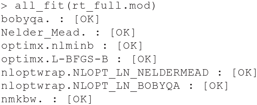
This output indicates that none of the optimizers tested led to convergence warnings or singular fits, both of which are indicative of problems with estimation. Thus, any of these optimizers should produce reliable parameter estimates.
In this example, our model converged when we changed the optimizer, but this will not always be the case, and you may sometimes need to address convergence issues in another way.
8
One option is to force the correlations among random effects to be zero. Recall that in addition to estimating fixed and random effects, mixed-effects models estimate correlations among random effects. If you are willing to accept that a correlation may be zero,
9
this will reduce the computational complexity of the model and may allow the model to converge on parameter estimates. Note, however, that it is advisable to conduct likelihood-ratio tests (described in detail in the next subsection) on nested models differing in the presence of the correlation parameter—or examine the confidence interval around the correlation—to determine whether elimination is warranted. To remove a correlation between two random effects in R, simply put a

Other ways to resolve convergence warnings include increasing the number of iterations before the model “gives up” on finding a solution (e.g.,
Finally, it may be that a model fails to converge simply because the random-effects structure is too complex (Bates, Kliegl, et al., 2015). In this case, one can selectively remove random effects based on model selection techniques (Matuschek et al., 2017). It is important to reiterate, however, that simplification of the random-effects structure should only be done as a last resort, and these decisions should be documented—the random-effects structure should be theoretically motivated, so it is best to try to maintain that structure unless all other methods of addressing convergence issues are unsuccessful.
Likelihood-ratio tests
Now that we have a model to work with, how do we determine if modality actually affected response times? This is typically done by comparing a model including the effect of interest (e.g., modality) with a model lacking that effect (i.e., a nested model) using a likelihood-ratio test. 10 This test is used to compare two nested models by calculating likelihoods for the two models using a technique called maximum likelihood estimation and then statistically comparing those likelihoods. If you obtain a small p value from the likelihood-ratio test, this indicates that the full model provides a better fit for the data.
When we run a likelihood-ratio test for our example, we are basically asking, does a model that includes information about the modality in which words are presented fit the data better than a model that does not include that information? Here is how you do this in R, first by building the reduced model that lacks the fixed effect for modality but is otherwise identical to the full model (including any control parameters used), and then by conducting the test via the
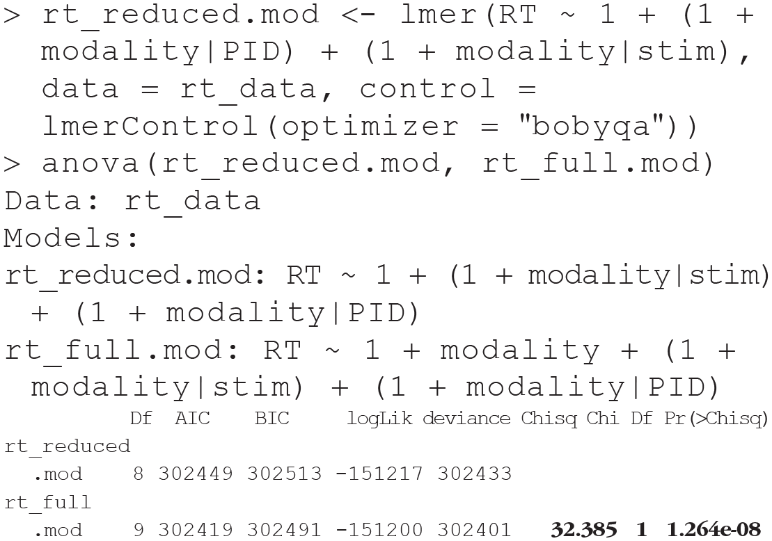
The small p value in the
Given that the full model includes only one condition effect (modality), conducting the test is relatively straightforward. However, performing likelihood-ratio tests can quickly become a tedious task for complex models with many fixed effects. This is because these tests must be conducted on nested models, so in order to test a particular effect, a reduced model (sometimes referred to as a null model) lacking that effect needs to be built for comparison. Another issue with this approach is that although the reduced models are built solely for the purpose of comparison with the full model, it can be quite tempting to examine those intermediate models and consider them plausible candidates for the “best model” (i.e., perform stepwise regression without knowing it). For example, suppose you build a full model with two fixed effects—modality and background-noise level—and a reduced model to test whether the effect of modality is significant. In doing so, you may notice that noise level is significant in the reduced model but not in the full model and convince yourself that a model without modality is actually more appropriate, even though you had not considered this possibility before examining the models. This is a questionable research practice (John et al., 2012) known as hypothesizing after the results are known (HARKing) and should be avoided because, as Kerr (1998) put it, HARKing transforms Type I error (false positives) into theory.
Luckily, the afex package has another handy function that allows you to avoid this practice altogether. The

Interpreting fixed and random effects
The likelihood-ratio test comparing our full and reduced models indicated that the modality effect was significant, but it did not tell us about the direction or magnitude of the effect. So how do we assess whether the audiovisual condition resulted in slower or faster response times? And how do we gain insight into the variability across participants and items that we asked the model to estimate? To answer these questions, we need to examine the model output via the

Recall that we used a dummy-coding scheme with the audio-only condition as the reference level; the intercept therefore represents the estimated mean response time in the audio-only condition, and the modality effect represents the adjustment to the intercept in the audiovisual condition. Thus, response times in the audio-only condition averaged an estimated 1,044 ms, and response times were an estimated 83 ms slower in the audiovisual condition.
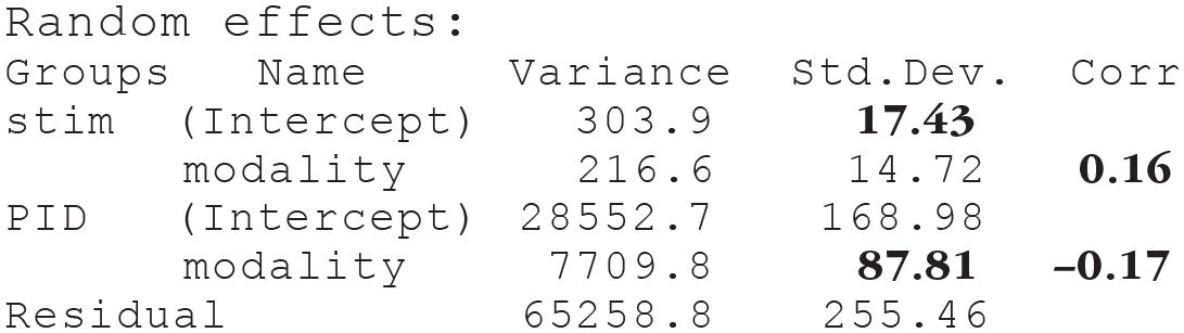
Now let us focus on the random-effects portion of the output:
The

This output indicates that the estimated intercept for the word “bag” is 1,043 ms, and the estimated slope is 86 ms; these values are very similar to the estimates for the fixed intercept (1,044 ms) and slope (83 ms). The participant part of the output indicates that Participant 303 had an estimated intercept of 883 ms and an estimated slope of 58 ms, indicating that this person responded much more quickly than average and was less affected by modality than average. Notice that even though we are looking at estimates for only four items and participants, it is clear that there is more intercept and slope variability across participants than across items. The standard deviations are consistent with this observation. Specifically, the standard deviations for the by-participant random intercepts (169 ms) and slopes (88 ms) are much larger than those for the by-item random intercepts (17 ms) and slopes (15 ms). This is not surprising—in my experience, participants tend to vary more than items—but it is useful to know that participants vary considerably in their response times because this could have important consequences for power calculations and could uncover avenues for individual differences research (e.g., why do people vary so much in the way the modality manipulation affects their response times?) and follow-up studies (e.g., do the results hold when one controls for individual differences in simple reaction time?).
Although the focus of our hypothetical study is on fixed effects, random-effects estimates can be interesting and informative in their own right, and in some cases provide insight into the key research question. For example, Idemaru and colleagues (2020) recently concluded that loudness is a more informative cue than pitch in predicting whether an utterance is perceived as respectful or not respectful. This claim was supported both by greater variation in pitch than loudness slopes across participants (i.e., participants responded more consistently to loudness cues) and by the fact that the direction of the loudness effect was negative for every single participant (this is an example of the
The last piece of information in the random-effects output concerns correlations among random effects. The
Finally, it is important to note that it is possible for a model to encounter estimation issues (i.e., produce unreliable parameter estimates) without any warning messages appearing in aggressive red text in your R console, and the random-effects portion of the output contains some clues that may help you identify when this happens. One clue comes from the random-effects correlations, which are set to −1.00 or 1.00 by default when they cannot be estimated, and another comes from the variance estimates, which are set to 0 when they cannot be estimated (i.e., the variance and correlation parameters are set to their boundary values when they cannot be estimated; Bates, Mächler, et al., 2015). Although random-effects correlations of −1.00 or 1.00 are often accompanied by “singular fit” warning messages, this is not always the case, so it is crucial to examine the random-effects portion of the model output to ensure that estimation went smoothly.
Reporting results in a manuscript
There are no explicit rules for reporting findings from model comparisons and the associated parameter estimates from the preferred model (Meteyard & Davies, 2020). How results are reported depends on the number and nature of model comparisons, the journal submission guidelines, and author and reviewer preferences. That said, I typically report the χ2 value from the likelihood-ratio test, the degrees of freedom of the test, and the associated p value, as well as the coefficient estimates, t values, and standard errors associated with the parameters of interest from the selected model. To report the findings described in the example above, you could write,
A likelihood-ratio test indicated that the model including modality provided a better fit for the data than a model without it, χ2(1) = 32.39, p < .001. Examination of the summary output for the full model indicated that response times were on average an estimated 83 ms slower in the audiovisual relative to the audio-only condition(
As long as you report your results transparently and include details of the model specification and any simplifications you made to the random-effects structure in your manuscript or accompanying code, the particular convention you follow is up to you (and, of course, making your data and code publicly available reduces the impact of the reporting convention you adopt). Finally, you should be sure to cite R as well as the specific packages you used to conduct your analyses, including the versions you used, both to facilitate reproducibility of your results (indeed, it is not uncommon for a model that once converged to no longer converge with an lme4 update) and to give credit to the package developers who have put a lot of work into making your analyses possible.
Interpreting interactions
The data set we have been working with throughout this Tutorial contains just one condition effect. Although this simplicity is convenient for learning about mixed-effects models, many experiments test multiple conditions and the interactions among them. Interpreting interactions is tricky, and doing so accurately depends critically on knowledge of the coding scheme used for categorical predictors. R’s default (and usually my own) is to use dummy coding, which leads to misinterpretation of interactions and lower-order effects if sum coding is assumed to be the default. Therefore, for this section, I continue to use dummy-coded predictors. The example I provide uses the same data set we have been working with, but contains one additional categorical predictor representing the difficulty of the background-noise level. Participants identified speech in audio-only (coded 0) and audiovisual (coded 1) conditions in both an easy (coded 0) and a hard (coded 1) level of background noise. The goal of this analysis is to assess whether the effect of modality on response time depends on (i.e., interacts with) the level of the background noise (i.e., the signal-to-noise ratio, or SNR). On the basis of previous research, we expect that response times will be slower in the audiovisual condition (as in the analyses above), but that this slowing will be more pronounced in easy listening conditions because the cognitive costs associated with simultaneously processing auditory and visual information are amplified in conditions in which seeing the talker is unnecessary to attain a high level of performance (see Brown & Strand, 2019).
There are a few ways to specify an interaction in R that produce identical results. One way is to use an asterisk

Another way to specify an interaction is to use a colon rather than an asterisk

Here is the abbreviated model output:

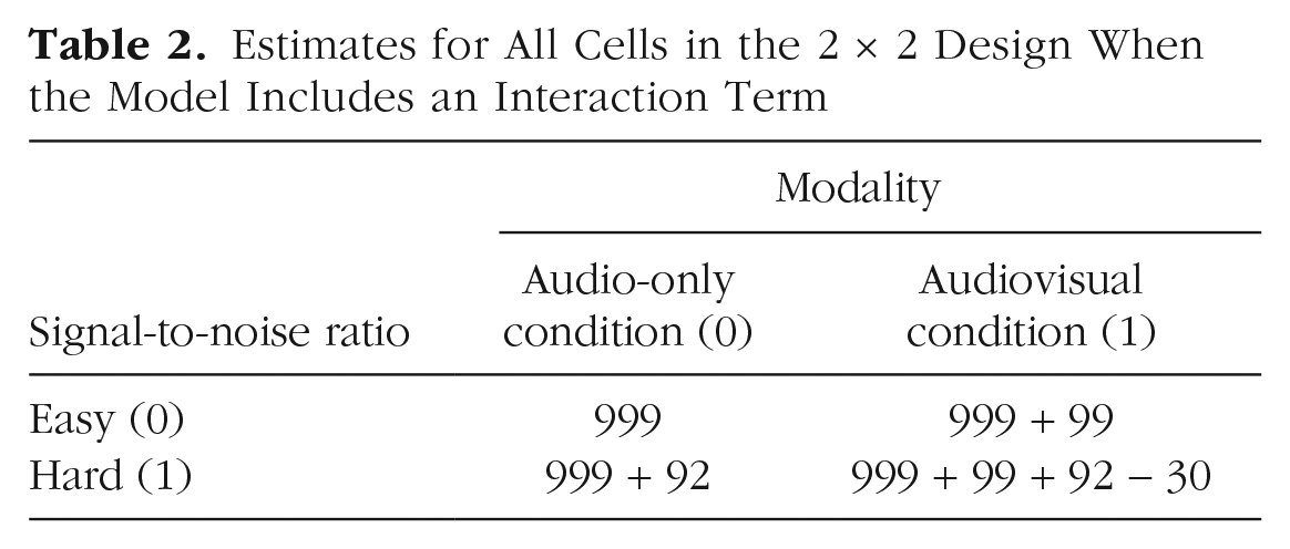
Recall that the intercept represents the estimated response time when all other predictors are set to 0. The intercept of 999 ms therefore represents the estimated mean response time in the audio-only modality (modality = 0) in the easy listening condition (SNR = 0). If you are having difficulty understanding why this is the case, it may be helpful to plug in 0 for both modality and SNR in the following regression equation. Notice that the intercept is the only term that does not drop out:

To interpret the remaining three coefficients, it is important to note that when an interaction is included in a model, it no longer makes sense to interpret the predictors that make up the interaction in isolation. This means that the coefficient for the modality term should not be interpreted as the average modality effect if SNR is held constant (this would be the interpretation if we had not included an interaction in the model), because the presence of the interaction tells us that the modality effect changes depending on the SNR. Instead, the coefficient for the modality term should be interpreted as the estimated change in response time from the audio-only to the audiovisual condition when all other predictors are set to 0. Thus, the modality effect indicates that response times are on average 99 ms slower in the audiovisual relative to the audio-only condition in the easy listening condition (SNR = 0). Think of it this way: When the SNR dummy code is set to 0 (easy), the SNR and interaction terms drop out of the model, and we are left with a 99-ms adjustment to the intercept when we move from the audio-only to the audiovisual condition. However, when the SNR dummy code is set to 1 (hard), those terms do not drop out of the model, and it is no longer accurate to say that the modality effect is 99 ms (again, plugging 0s and 1s into the regression equation above may help you here).
Similarly, the SNR effect indicates that response times are on average 92 ms slower in the hard relative to the easy listening condition, but this applies only when the modality dummy code is set to 0 (representing the audio-only condition). The modality and SNR effects I have just described are called simple effects, but are often misinterpreted as main effects. Simple effects represent the effect of a predictor on an outcome at a particular level of another predictor, whereas main effects represent the average effect of a predictor on an outcome across levels of another predictor. Thus, when an interaction is present and you have used a coding scheme centered on 0 (e.g., sum coding), lower-order effects are considered main effects, but if you have used a dummy-coding scheme, they are simple effects. Keep this common misinterpretation in mind any time you use dummy coding.
Just as the modality and SNR effects can be thought of as adjustments to the intercept in particular conditions (e.g., estimates are shifted up 99 ms in the audiovisual relative to the audio-only condition, but only in the easy listening condition), the interaction term can be thought of as an adjustment to the modality or SNR slope when both predictors are set to 1 (note that interactions adjust coefficient estimates only for a single cell of the design because the interaction term drops out when one or both of the predictors are set to 0). In this example, the coefficient for the modality term indicates that the modality effect is 99 ms when the SNR is easy, but the presence of an interaction tells us that the effect of modality differs depending on the level of the background noise; that is, the modality slope needs to be adjusted when the SNR is hard. Specifically, the negative interaction term indicates that the modality slope is 30 ms lower (less steep) when the SNR is hard, which is consistent with the hypothesis I described above: Seeing the talker slows response times, but it does so to a greater extent when the listening conditions are easy, presumably because the visual signal is distracting and unnecessary when the auditory signal is highly intelligible. Note that interactions are symmetric in that if the modality slope varies by SNR, then the SNR slope varies by modality. You can therefore also interpret the interaction term as an adjustment to the SNR slope: The 92-ms SNR effect is 30 ms weaker in the audiovisual condition. If you are struggling to interpret interactions with dummy-coded predictors, I recommend making a table containing the coefficient estimate for each of the cells in the design by plugging all combinations of 0s and 1s into the regression equation (Table 2); this can help you visualize the role of each individual coefficient estimate in generating cell-wise predictions (see also Winter, 2019).
Estimates for All Cells in the 2 × 2 Design When the Model Includes an Interaction Term
Analyzing data with a binary outcome (identification accuracy)
Now you should have a general understanding about how to build and interpret models in which the outcome is continuous (e.g., response time), but what if you wanted to test for an effect of modality on accuracy at identifying words, when accuracy for each trial is scored as 0 or 1? These values are discrete and bounded by 0 and 1, so you need to use generalized linear mixed-effects models; if we instead modeled this discrete outcome assuming a continuous outcome, the model would generate impossible predictions (e.g., a predicted probability of −0.2 or 1.3). The R code for building these kinds of models is almost exactly the same as that described above, except rather than using the
Put simply, the logit link function first transforms probabilities, which are bounded by 0 and 1, into odds, which are bounded by 0 and infinity (a probability of 0 corresponds to odds of 0, and a probability of 1 corresponds to odds of infinity). However, this scale still has a lower bound of 0, so the link function takes the natural logarithm of the odds (the logarithm of 0 is negative infinity, so the lower bound of the scale is extended from 0 to negative infinity), which results in the continuous and unbounded log-odds scale. Using this function means that any predictions generated from the model will also be on a log-odds scale, which is not particularly informative, but luckily, these predictions can be exponentiated to put them back on an odds scale, and the odds can then be converted into probabilities (see Jaeger, 2008, for a tutorial on using logit mixed models).
Here is the code to build the full model:

This code is very similar to that for the response time analysis, but it contains a few key differences. First, the dependent variable is
This model converged, but remember that you should always examine the random-effects portion of the output to ensure that estimation went smoothly:

Not only did we not encounter any convergence or singularity warnings, but the variance estimates and estimated correlations among random effects seem reasonable (i.e., the variance estimates are not exactly zero, and the correlations are not −1.00 or 1.00). It is slightly unusual that in this data set there is more variability across items than across participants in both intercepts and slopes, but this may simply reflect the fact that the speech-identification task was relatively easy for most participants, which resulted in little variability. 12
Next, we will build a reduced model lacking modality as a fixed effect so we can conduct a likelihood-ratio test:

It is important to note that although both the full and reduced models converged with this random-effects structure and no control parameters, it is certainly possible (and indeed not uncommon) for the full model to converge but the reduced model to encounter convergence issues. In this case, you should find a random-effects structure and combination of control parameters that enable both models to converge (e.g., via the
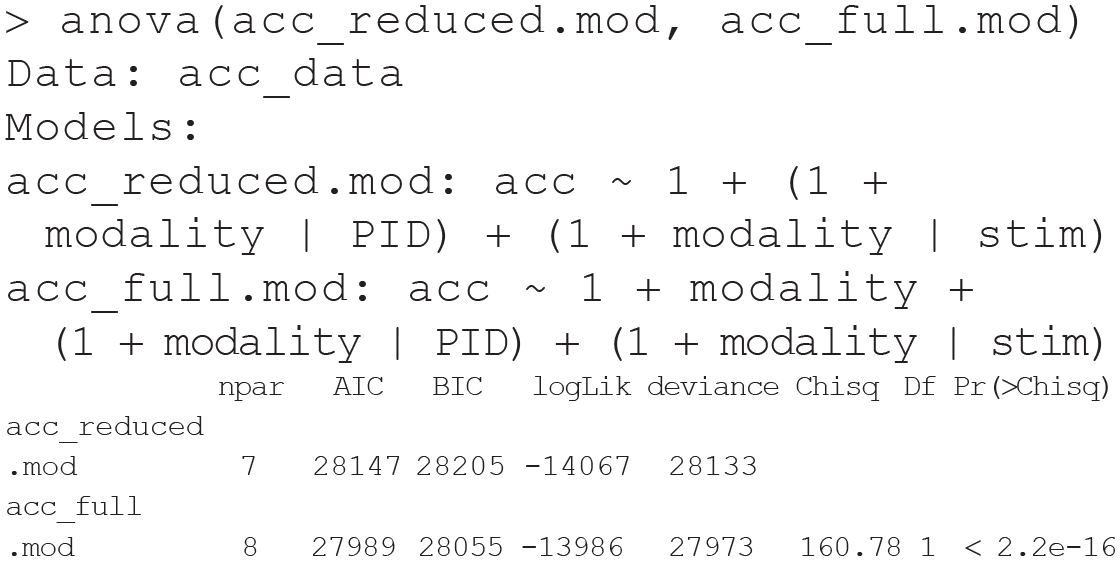
The small p value indicates that the full model provides a better fit for the data than the reduced model, and thus that modality has a significant effect on spoken-word identification accuracy.
Conclusions
Mixed-effects modeling is becoming an increasingly popular method of analyzing data from experiments in which each participant responds to multiple items—and for good reason. The beauty of mixed-effects models is that they can simultaneously model participant and item variability while being far more flexible and powerful than other commonly used statistical techniques: They handle missing observations well, they can seamlessly include continuous predictors, they provide estimates for average (as well as by-participant and by-item) effects of predictors on the outcome, and they can be easily extended to model categorical outcomes.
However, as Uncle Ben once said to Spider-Man, with great power comes great responsibility (Lee & Ditko, 1962). These models can be easily implemented in R without cost, but it is important that researchers ensure that this powerful tool is used correctly. Indeed, although more and more researchers are implementing mixed-effects models, there is a concerning lack of standards guiding implementation and reporting of these models (Meteyard & Davies, 2020). Many analytic decisions must be made when using this statistical technique. Consider, for example, the number of options available to the researcher if a model fails to converge. This results in a massive number of “forking paths” (Gelman & Loken, 2014) that the researcher may embark upon to obtain statistically significant results. Given the considerable number of choices a researcher may make during data analysis (i.e., researcher degrees of freedom; Simmons et al., 2011), it is important that these models be used carefully and reported transparently (see Meteyard & Davies, 2020, for an example of how models and results should be reported).
The goal of this article is to serve as an accessible, broad overview of mixed-effects modeling for researchers with minimal experience with this type of modeling. I have focused on what mixed-effects models are, what they offer over other analytic techniques, and how to implement them in R. Table 3 lists helpful links, as well as additional resources for readers interested in more in-depth descriptions of particular topics.
Helpful Links and Additional Resources

Footnotes
Acknowledgements
I am grateful to Michael Strube for providing detailed feedback on an earlier draft of the manuscript and to Julia Strand and Kristin Van Engen for providing helpful comments and suggestions throughout the writing process.
Transparency
Action Editor: Mijke Rhemtulla
Editor: Daniel J. Simons
Author Contributions
V. A. Brown is the sole author of this article and is responsible for its content. She devised the idea for the article, wrote the article in its entirety, wrote the accompanying R script, and generated the dummy data on which the models are based.