Persons as Effect Sizes

Abstract

Traditional indices of effect size are designed to answer questions about average group differences, associations between variables, and relative risk. For many researchers, an additional, important question is, “How many people in my study behaved or responded in a manner consistent with theoretical expectation?” We show how the answer to this question can be computed and reported as a straightforward percentage for a wide variety of study designs. This percentage essentially treats persons as an effect size, and it can easily be understood by scientists, professionals, and laypersons alike. For instance, imagine that in addition to d or η², a researcher reports that 80% of participants matched theoretical expectation. No statistical training is required to understand the basic meaning of this percentage. By analyzing recently published studies, we show how computing this percentage can reveal novel patterns within data that provide insights for extending and developing the theory under investigation.

The American Statistical Association’s Symposium on Statistical Inference and subsequent summary publication “Moving to a World Beyond ‘p < 0.05’” (Wasserstein, Schirm, & Lazar, 2019a) serve as recent indicators of the decline of null-hypothesis significance testing (NHST) in the social and life sciences. In its place, scholars and statisticians have developed alternative methods for drawing inferences in regard to population parameters, such as the estimation (Cumming, 2014), a priori (Trafimow, 2019), and statistical-sameness (Hubbard, 2016) approaches, among others (see Wasserstein, Schirm, & Lazar, 2019b). Efforts to reduce scientists’ reliance on NHST began to gain traction in the 1990s, most notably with the published findings of the American Psychological Association’s task force on significance testing (Wilkinson & Task Force on Statistical Inference, American Psychological Association, Science Directorate, 1999). Simultaneously, interest in effect sizes also grew. Whereas NHST is used to draw inferences to population parameters from sample statistics, effect sizes are used to convey the magnitude of a given result, usually in terms of group differences or associations between variables. Consequently, effect sizes are often considered to be more relevant than NHST for judging the theoretical, practical, or clinical importance of a given study. Since the 1990s, numerous articles and book chapters on effect sizes have been published, and the number of available indices has grown to accommodate different types of variables, research designs, and statistical analyses. Kirk (1996), for instance, presented over two dozen effect-size indices, which he classified into measures of group differences, association, and relative risk (ratios). Huberty (2002), Rosnow and Rosenthal (2003), and Ferguson (2009a) followed suit, using similar classification schemes in their extensive summaries of effect sizes.

In this article, we bring together a number of ideas and methods, published over the past 70 or more years, for treating persons as effect sizes. Instead of conveying magnitudes regarding group differences or associations between variables, these person-centered effect sizes answer the general question, “How many people in the study behaved or responded in a manner consistent with theoretical expectation?” With the introduction of his nonparametric dominance statistics, Cliff (1993) argued that this is the type of question many researchers have in mind when designing and executing their studies. Grissom (1994) similarly argued that clinical psychologists are interested in answering a parallel question, namely, “How many people show superior outcomes undergoing one form of therapy compared with another?” The methods used to answer these questions draw on well-known nonparametric procedures that are easy to compute and understand and easily generalized to a wide variety of research designs and types of variables. Using open-source data from several studies, three published recently in Psychological Science, we followed Kirk’s (1996) classification scheme to demonstrate how these person-centered effect sizes can be derived for hypotheses regarding group differences (both within and between groups), associations, and relative risk.

Within-Person Differences

The question “How many people behaved in a manner consistent with theoretical expectation?” can be asked in the context of both within- and between-persons study designs, in which measures of central tendency are often compared. With respect to the former, consider the recent study by E. H. Siegel, Wormwood, Quigley, and Barrett (2018), in which the impact of suppressed affective expressions on the perception of neutral faces was examined. Using a technique called continuous flash suppression, Siegel and colleagues showed 45 participants a neutral face in full contrast to the dominant eye and an affective face in low contrast to the nondominant eye. The affective faces were smiling, neutral, or scowling and were labeled as the positive, neutral, and negative levels, respectively, of a repeated measures factor. Each participant viewed 180 pairs of faces and rated the neutral image shown to the dominant eye on a scale from 1 (scowling) to 5 (smiling). Consistent with theoretical expectation, mean affective ratings—the dependent variable—revealed that participants perceived neutral faces as more smiling when those faces were paired with suppressed positive faces and as more scowling when they were paired with suppressed negative faces. The omnibus repeated measures analysis of variance was statistically significant, F(2, 43) = 9.72, p < .001, as were all pairwise differences between the three levels (positive, neutral, and negative) of the independent variable (ps < .05). With regard to effect size, Siegel and colleagues reported η² equal to .32 and a Bayes factor equal to 62.9. The former value indicates a large effect according to Cohen’s (1988) conventions or a moderate effect according to Ferguson’s (2009a) conventions, and the latter value was interpreted by Siegel and colleagues as indicating “very strong evidence” (p. 499) in favor of their hypothesis.

We return now to the person-centered effect-size question: How many of the 45 participants in E. H. Siegel et al.’s (2018) study showed consistent decreases in their ratings across the three affective conditions? In other words, how many participants’ mean ratings matched the expected ordinal pattern: positive > neutral > negative? Examination of the results, which are freely available on OSF (http://osf.io/by9t3/), revealed that only 11 of the 45 participants, or 24.44%, matched this pattern. In this article, we refer generically to the percentage of participants whose responses matched expectation as the percent correct classifications (PCC ), and it can be regarded as a person-centered effect size. The top panel of Figure 1 shows the mean affective ratings for the 11 participants who matched expectation, and the middle panel shows the ratings for the five people whose pattern of mean responses were exactly the opposite of expectation. The bottom panel of Figure 1 shows the ratings for the remaining 29 participants, who did not match the expected ordinal pattern completely. ¹

Fig. 1.

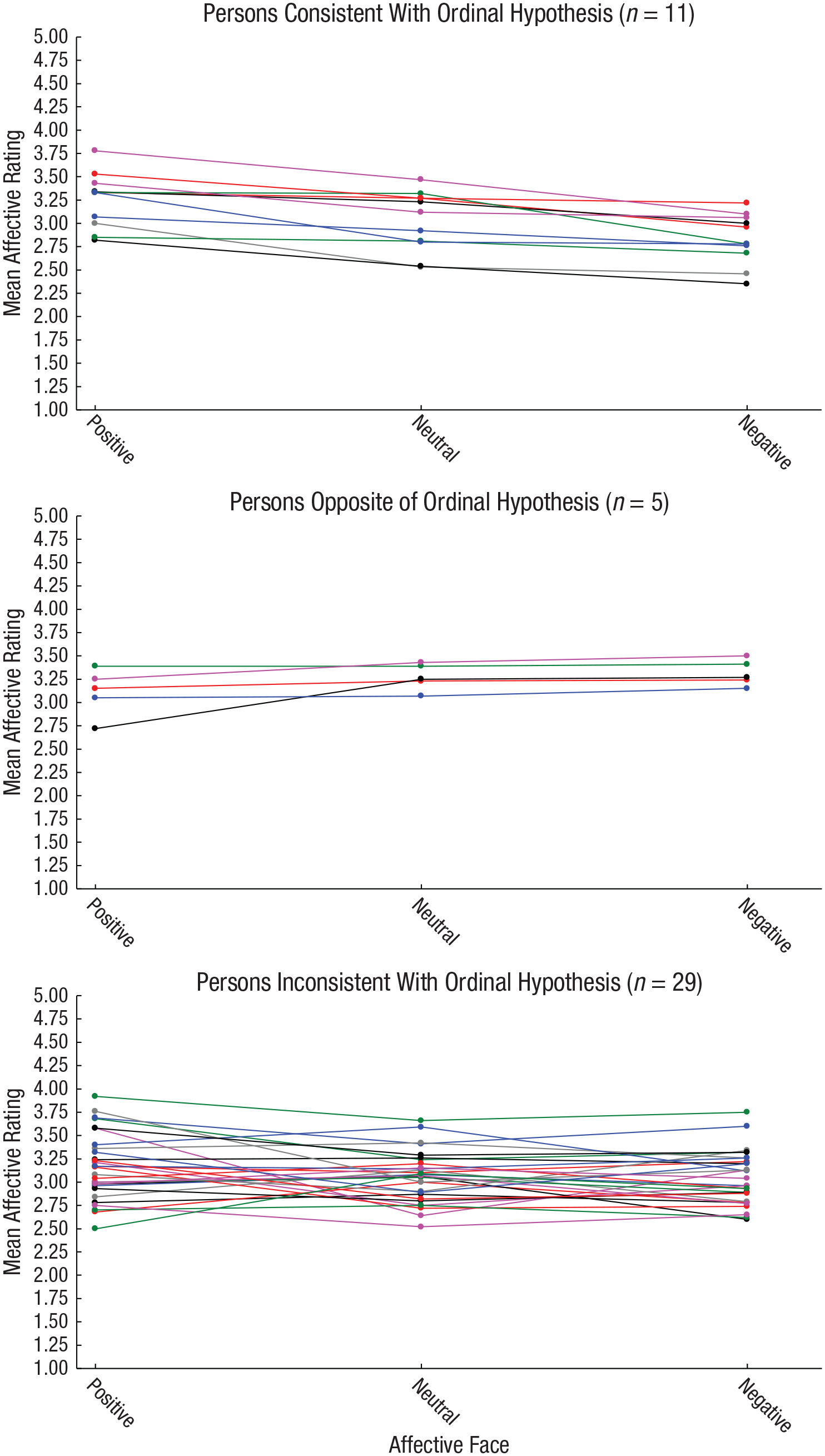
Results from E. H. Siegel, Wormwood, Quigley, and Barrett (2018): mean affective ratings of the positive, neutral, and negative face images for three groups of participants defined by their ordinal patterns.

The magnitude of the person-centered effect size, the PCC, is unimpressive, as a majority of participants (75.56%) rated the three affective stimuli in ways that contradicted the hypothesis. In contrast, the η² and Bayes-factor values are impressively high, indicating at least a moderate effect size using standard conventions and strong evidence in support of E. H. Siegel et al.’s (2018) hypothesis, respectively. At first glance, this inconsistency between the person-centered and aggregate effect sizes may seem perplexing or perhaps discouraging; however, as Fisher, Medaglia, and Jeronimus (2018) recently discussed, the ecological fallacy is a real and constant threat to drawing valid conclusions. Statistical inferences drawn from groups of individuals may not accurately describe the individuals themselves (see also Lamiell, 2013; Molenaar, 2004). This same reasoning applies to effect sizes, which means the η² and Bayes-factor values do not present a complete picture of the results—the person-centered effect sizes are also needed.

Moreover, pairwise PCCs suggest one way to strengthen and advance this line of research. The PCC was highest for the comparison of the negative and positive conditions; 71.11% of the participants’ mean ratings matched the expected pattern (positive > negative). This effect size exceeded those for the positive-neutral (PCC = 57.78%) and negative-neutral (PCC = 55.56%) comparisons. Because causes operate at the level of the individual, future research may yield more impressive PCCs by increasing the positivity and negativity of the affective expressions in the images presented to the nondominant eyes of the participants. A second way to advance this line of research would entail conducting similar ordinal analyses on individual responses to each of the unique pairs of images. The analyses we have presented were conducted on responses that were aggregated across trials of varying pairs of images, as were the analyses in the original study. By conducting more finely tuned analyses on individual responses, the efficacy of each image pair can be evaluated, much as a sample of data can be analyzed for outliers or influential cases. Finally, a third way of advancing this line of research is suggested by Figure 1: The five contrary participants—missed entirely by the analysis of variance—could be examined for a quality that may operate as a moderator variable. In other words, there may be some common and theoretically meaningful quality that contributed to these individuals’ opposite pattern of mean ratings.

It is important to emphasize that all of these suggestions, as well as those in the examples we present later, must be considered as applying to future studies, ideally under the guide of theory. Simply seeking to increase a PCC is no better than obsessively focusing on reducing the magnitude of a p value, and such an outlook also puts the researcher at grave risk of generating biased results. Caution must particularly be exercised when ad hoc analyses are conducted within a given study, such as when researchers attempt to control for posttreatment variables or assess the impact of influential cases identified by posttreatment criteria (see Montgomery, Nyhan, & Torres, 2018).

Between-Group Differences

For between-participants designs, the simplest way to compute the person-centered PCC index is to take the idea of comparing groups and apply it to individuals. Consider, for example, the recent study by Sawaoka and Monin (2018, Study 1; data available at https://osf.io/qtsx2/) in which participants viewed an offensive media post and then read fictitious comments that expressed moral outrage at the post. Participants were divided into nonviral and viral groups; the nonviral group read 2 comments, and the viral group read 10. Participants were then asked to evaluate one of the commenters (selected by the authors) for the following characteristics: “in the wrong,” “a bully,” “praiseworthy,” and “a good person” (response scale from 1 to 7). The four items were keyed so that the scale was in the same direction for all of them, and responses were averaged to form the primary dependent variable for the study; high scores indicated a negative evaluation. Sawaoka and Monin theorized that the commenter evaluated in the viral, 10-comment condition would be seen as someone seeking social validation rather than as someone expressing authentic moral outrage. Consequently, they predicted that the evaluations would be more negative in the viral condition compared with the nonviral condition. The mean magnitudes and results from their analysis of variance supported this prediction, F(1, 377) = 8.51, p = .004, d = 0.29.

A person-centered PCC effect size can be computed by comparing pairs of individuals from the two groups on the dependent variable. Specifically, the evaluation rating of each person in the viral group (n = 198) can be compared with the evaluation rating of each person in the nonviral group (n = 192), for a total of 38,016 comparisons. Given Sawaoka and Monin’s (2018) hypothesis, a comparison is counted as a correct classification if the rating provided by the person in the viral group is greater than the rating provided by the person in the nonviral group (i.e., viral > nonviral). This procedure is analogous to the Mann-Whitney U test (see Grissom, 1994; Ruscio, 2008), except that ties are treated as incorrect classifications. Results for the 38,016 comparisons revealed that just over half (20,753) of the pairs of individual ratings met expectation, indicating that the two groups of individuals were not easily distinguishable (PCC = 54.59%). In other words, across all possible comparisons of two participants from the different groups, the evaluative rating in the viral condition was higher than the evaluative rating in the nonviral condition only a slight majority of the time.

Sawaoka and Monin (2018) conducted five extended replication studies testing their hypothesis. All of the results were statistically significant, and the mean ratings were consistent with expectation. Effect sizes were reported as Cohen’s d values that ranged from 0.14 to 0.35 in magnitude (see Table 1). Sawaoka and Monin interpreted these values as indicating medium effects. We computed the person-centered PCC effect sizes for the additional five studies, and the results are reported in Table 1. As can be seen, the PCC values ranged from 45.79% to 56.40%. When two groups are compared, a PCC equal to 50% might be expected by chance. Given this benchmark, the results for all six studies are not very impressive. Strikingly, the largest d value, in Study 5, was paired with the smallest PCC index. The reason for this discrepancy is that Sawaoka and Monin created the primary dependent variable in this study from only two rated items, “in the wrong” and “a bully.” The resulting histograms for the viral and nonviral groups were positively skewed, and their high degree of overlap resulted in the low PCC. Parametric statistical analysis and Cohen’s d, both based on means and standard deviations, are not appropriate for such data.

Table 1.

Sample Sizes, Cohen’s ds, and Percent Correct Classification (PCC) for Sawaoka and Monin’s (2018) Six Viral-Outrage Studies

Study	N	Ordinal prediction (viral > nonviral)
		d	PCC
1	390	0.29	54.59
2	587	0.29	56.40
3	590	0.21	53.60
4a	799	0.25	50.87
4b	769	0.14	51.14
5	179	0.35	45.79

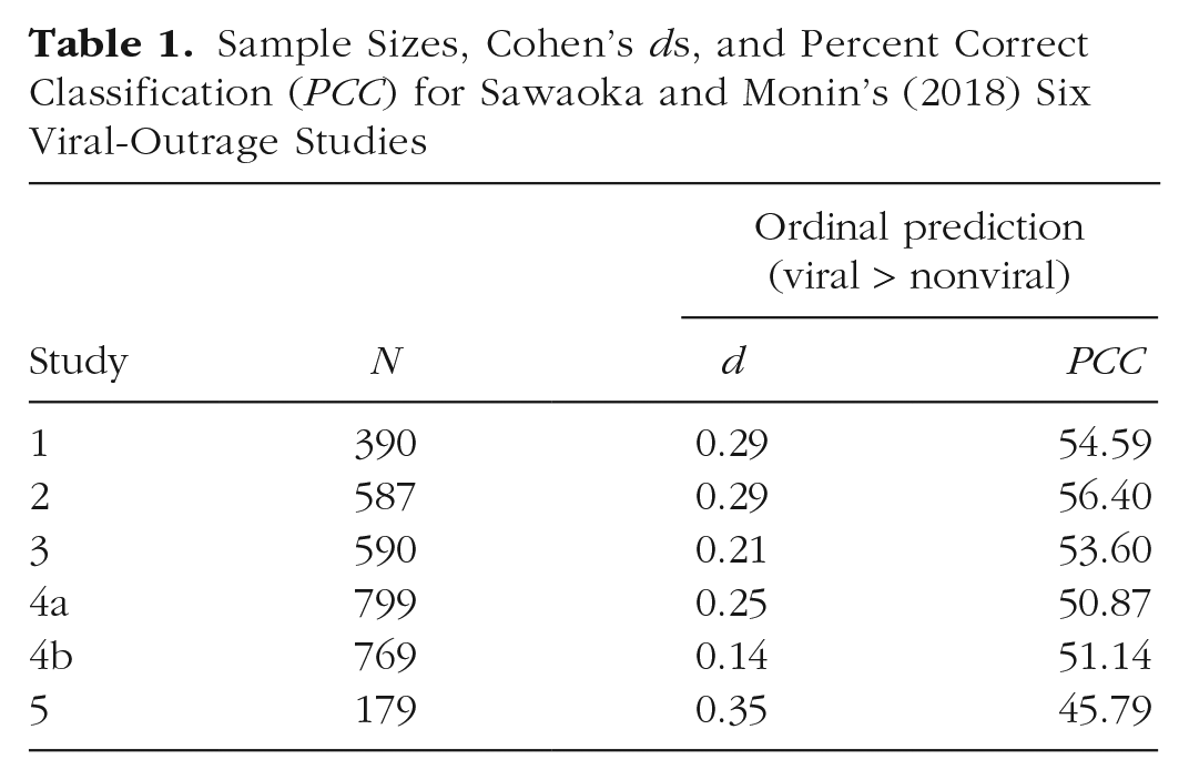
Sawaoka and Monin (2018, p. 1666) argued that the effect sizes could likely be increased by requiring participants to read more than 10 posts in the viral condition. The person-centered effect sizes suggest that such efforts are warranted as a way to advance and strengthen this line of research, to potentially provide more convincing evidence for the viral-outrage phenomenon. Perhaps a more important implication of the PCC indices in Table 1 is that the dependent variable should be scrutinized more carefully. After two items were dropped from the composite that formed the dependent variable in Study 5, the PCC dropped below 50%. Sawaoka and Monin reported Cronbach’s alpha values greater than .80 for the items that were averaged to create the dependent variable, but the items may have tapped into sufficiently different qualities to warrant caution against their aggregation.

Associations Between Variables

Correlation and regression analyses that examine linear relationships between and among variables have long been a staple of scientific research. Consider the recent study by Geniole et al. (2019; data available at https://osf.io/3jhr7/), in which they examined the impact of testosterone, personality, and genes on aggression in males. Two groups of men received a nasal gel containing either 11 mg of testosterone or a placebo. The men also completed a self-report questionnaire that assessed risk for testosterone-induced aggression (personality risk), provided a saliva sample for genetic assessment (cytosine-adenine-guanine, CAG, repeats in exon 1 of the androgen receptor gene), and participated in a competitive online game against a confederate as an assessment of behavioral aggression. Geniole and colleagues examined the relationship among these variables using a form of regression that is robust to influential cases. Specifically, they regressed the behavioral-aggression scores onto group membership (placebo vs. testosterone), personality risk, and CAG repeat length (i.e., number of repeats), as well as their interactions. The two largest statistical effects to emerge from the regression analysis were the main effect of personality-risk score, b = 1.515, t(300) = 2.603, p = .010, d = 0.301, and the effect of the three-way interaction, b = −2.681, t(300) = −2.667, p = .008, d = −0.308. Higher risk scores were predictive of greater behavioral aggression, and a breakdown of the interaction showed that the effect of testosterone was greatest for those individuals with high risk scores (+1 SD) and low values of CAG repeat length (−1 SD), b = 8.691, t(300) = 4.420, p < .001, d = 0.510.

The behavioral-aggression dependent variable ranged in value from 0 to 53.33 and was calculated as the number of times the participant attempted to steal points from the confederate divided by the number of times the participant was provoked in the game. The personality-risk (range: −1.72–2.22) and CAG-repeat-length (range: 10–30) independent variables were similarly constituted as real or whole numbers. Consequently, these three variables must be binned in some manner to derive person-centered effect sizes like those described in the previous examples. A median split of each variable may raise red flags for researchers familiar with the problems inherent in dichotomizing variables, particularly those associated with changes in Type I error rates (Maxwell & Delaney, 1993; Vargha, Rudas, Delaney, & Maxwell, 1996). The goal here, however, is purely descriptive, to answer the question, “How many men in Geniole et al.’s (2019) study can be classified correctly on the basis of the predictions and regression results?” The most important potential problem for dichotomizing or binning in this context, then, is information loss, which can be addressed by attending to the variables’ distributions. As can be seen in Figure 2, for instance, the behavioral-aggression dependent variable was radically skewed (z_skew = 10.75). A notable fact not revealed by the regression analyses is that 52 of the 308 men (17%) scored zero on this variable, which means they did not attempt to steal a single point from their opponent in the online competition. No other value for the dependent variable, recorded to two decimals of precision, was observed for more than six men (see Fig. 2).

Fig. 2.

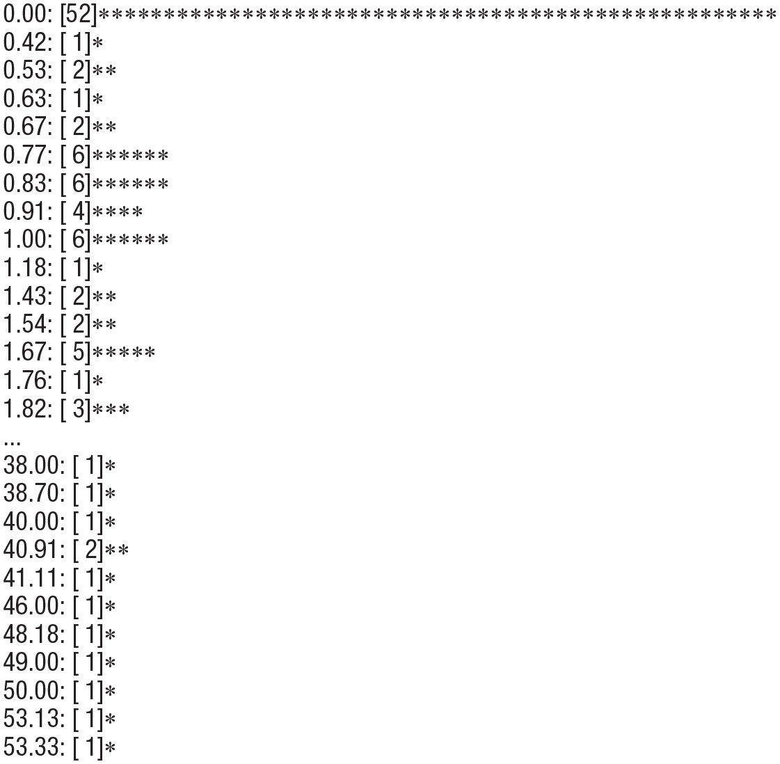
Partial list of frequencies for the behavioral-aggression dependent variable in Geniole et al. (2019). Each asterisk represents one person, and frequencies are reported in brackets.

Are these 52 men qualitatively, rather than quantitatively, different from their cohort? Taking this to be a real possibility, we binned them into their own group, and the remaining 256 men were then divided into two additional groups based on a median split of their responses. The binned distribution is shown in Figure 3.

Fig. 3.

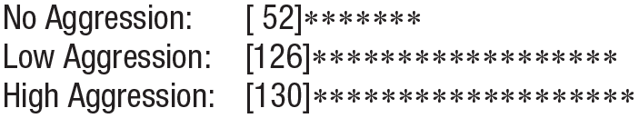
Frequency histogram for the binned behavioral-aggression variable in Geniole et al. (2019). Each asterisk represents approximately seven people, and actual frequencies are reported in brackets.

The top predictor variable, personality risk, followed an approximate normal distribution with modest positive skew (z_skew = 2.37, z_kurtosis = 1.90) and was therefore dichotomized at the median. We then crossed the two binned variables and classified the aggression scores as correct or incorrect using a naive Bayesian classifier (Sauer, 2018). Figure 4a shows the results. Overall, only 48.70% of the men were classified correctly. The conditional proportions shown in the figure reveal that, consistent with the regression results, men with relatively high-risk personality scores were more likely to be aggressive compared with those with low-risk scores. Interestingly, the 52 men who did not attempt to steal a single point from their opponents in the online game—who showed no behavioral aggression—were equally distributed across the two personality types and therefore classified ambiguously. When these men were excluded from the analysis, the PCC increased to 58.59% (150/256), a more impressive although still modest effect size if one uses 50% as a baseline for classifying two groups.

Fig. 4.

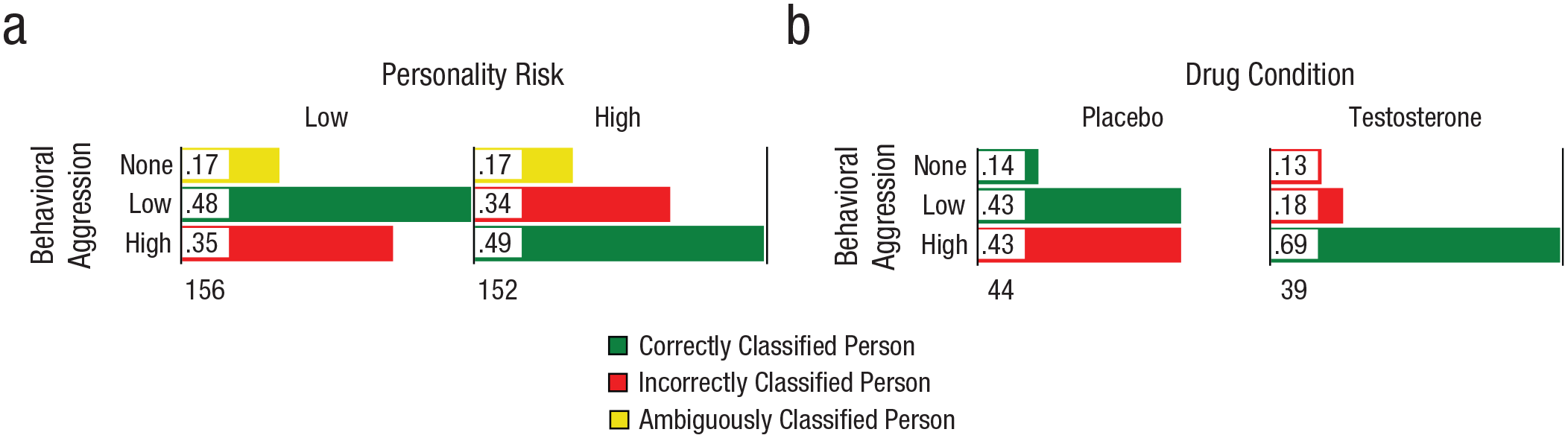
Results of applying a Bayesian classifier to the data for participants in Geniole et al.’s (2019) study. The graphs in (a) show the results for classification of all 308 men based on binned behavioral aggression crossed with binned personality risk. The graphs in (b) show the results for classification based on binned behavioral aggression crossed with drug condition. Only men with high personality-risk scores and low values of cytosine-adenine-guanine repeat length (n = 83) were included in the latter analysis. Conditional proportions are reported in the bars, and column totals are reported below the histograms.

To break down the three-way interaction, which yielded the largest Cohen’s d effect size, Geniole and colleagues (2019) conducted conditional regression analyses for combinations of low (−1 SD) and high (+1 SD) scores on the personality-risk and CAG-length variables. Results revealed that the statistical effect of drug group was largest for men with low CAG length and high personality risk, d = 0.510. Moreover, the d values for the remaining three combinations of low and high values were all below 0.050 in absolute magnitude. The impact of testosterone on behavioral aggression was therefore greatest for men with relatively high-aggression-risk personalities and low values of CAG repeat length.

We computed the person-centered effect size by binning (dichotomizing) the personality-risk and CAG-length variables according to median splits and then crossing the bins. The men in the low-CAG-length/high-personality-risk crossed bin (n = 83) were then analyzed. Figure 4b shows the classification results and conditional proportions. The PCC index was 62.65%, and results indicated that an impressively high percentage of men in the testosterone condition (69%) were also above the median (ignoring scores of zero) for the behavioral-aggression measure. Among men in the placebo group, the conditional proportions were equal (.43) for those above and below the median. The conditional proportions for those men who did not attempt to steal a single point from their opponents (n = 11) were nearly equal for the placebo (.14) and testosterone (.13) groups.

The person-centered effect sizes for Geniole et al.’s (2019) study thus offer additional information regarding the impact of testosterone on behavioral aggression. They also reveal patterns in the data missed by traditional analyses and suggest that one possible route for advancing this line of research is to pay special attention to men who show no signs of aggression. These men may not be strictly quantitatively different from other men in terms of aggressiveness in a competitive game. Therefore, treating the behavioral-aggression score as strictly continuous in correlation or multiple regression analyses may fail to capture important and theoretically relevant individual differences.

Risk Assessment

Testosterone levels were assessed by Geniole et al. (2019) after all experimental tasks were completed, providing data for ensuring that men assigned to the drug group possessed higher levels of the hormone than those who received a placebo. We used the testosterone levels to separate the men (n = 307 because of one missing value) into two groups according to a median split. This dichotomous variable was then crossed with the group variable (drug vs. placebo), and the individual observations were categorized using a naive Bayesian classifier. As can be seen in Figure 5, 92.51% of the men were classified correctly and in a manner consistent with expectation. The conditional percentages were also extremely impressive. Ninety-two percent of the men who received placebo were below the median testosterone value, whereas 93% of the men who received testosterone were above the median.

Fig. 5.

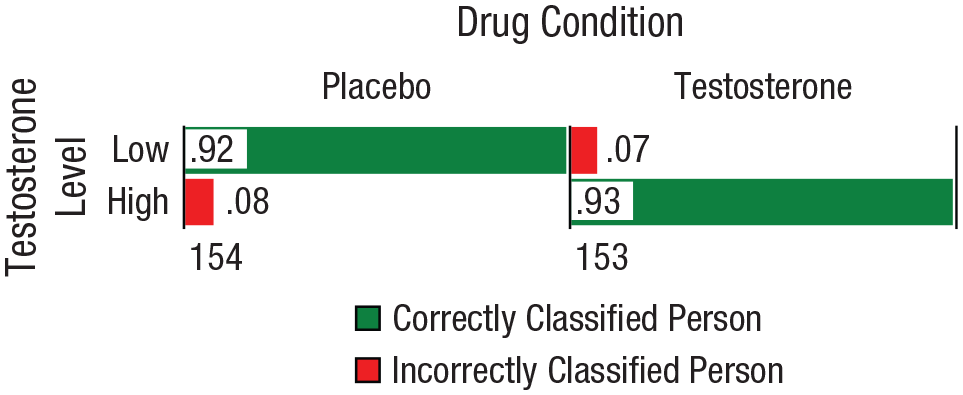
Results of applying a Bayesian classifier to the testosterone data from participants in Geniole et al.’s (2019) study. The graphs show the results for classification of 307 men based on drug condition and binned testosterone level (median split) following the experimental procedure. Conditional proportions are reported in the bars, and column totals are reported below the histograms.

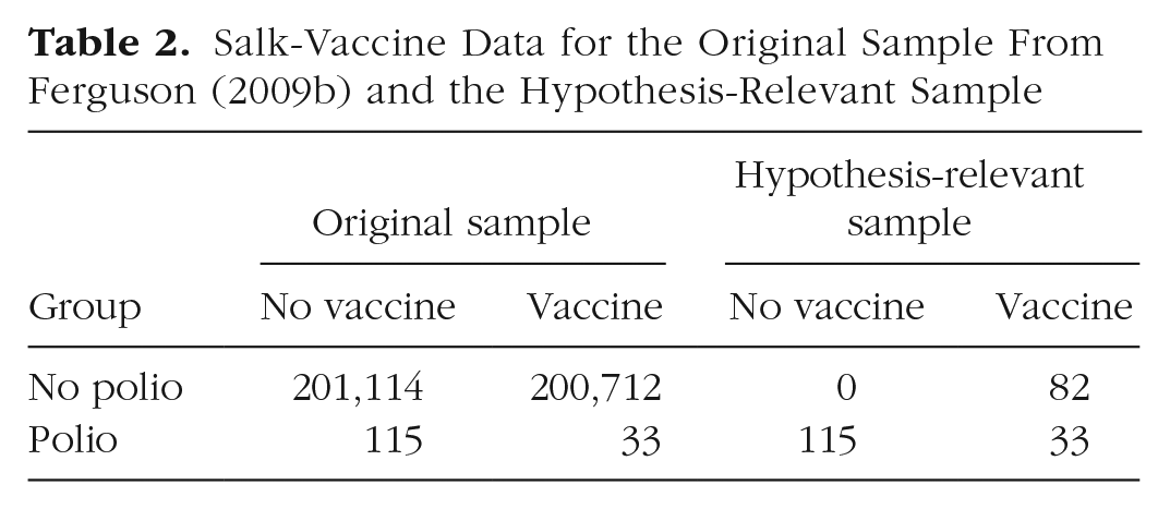
For Geniole et al.’s (2019) study, the men were randomly assigned to the two drug groups with equal frequency. Similarly, a median split of the measured testosterone levels created two groups with nearly equal sample sizes. In nonexperimental studies, particularly epidemiological research, different groups may differ radically in sample size, which leads to difficulties in interpreting effect sizes. To provide an example of these challenges, Ferguson (2009b) reprinted data on the Salk vaccine that Rosnow and Rosenthal (2003) had used to argue that even small correlations can be interpreted as providing convincing evidence for an effect. After all, the Salk vaccine is known to be effective, yet in the original sample, the correlation between receiving or not receiving the vaccine and the incidence of polio (see Table 2) was surprisingly small, r = .011. Similarly, as shown in Figure 6, the PCC for this sample is only 49.96%—essentially a 50/50 split—though the conditional proportions for children with polio are smaller among those who received the vaccine (.00016) compared with those who did not receive the vaccine (.00057).

Table 2.

Salk-Vaccine Data for the Original Sample From Ferguson (2009b) and the Hypothesis-Relevant Sample

Group	Original sample		Hypothesis-relevant sample
	No vaccine	Vaccine	No vaccine	Vaccine
No polio	201,114	200,712	0	82
Polio	115	33	115	33

Fig. 6.

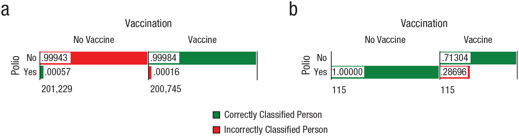
Polio incidence among individuals who did and did not receive the Salk vaccine (Ferguson, 2009b). Results are shown for (a) all 401,974 children in the original sample and (b) only children considered hypothesis relevant (n = 230). Conditional proportions are reported in the bars, and column totals are reported below the histograms.

Ferguson (2009b) argued, however, that most of the original-sample data in Table 2 are not strictly hypothesis relevant because of the “cast the net wide” (p. 132) sampling methods used. He considered the original hypothesis to be “The Salk vaccine is effective in preventing polio in individuals who are exposed to the polio virus” (p. 132). He then used the proportion of children in the unvaccinated group who contracted polio (115/201,229 = 5.71 × 10⁻⁴) as a base rate for the vaccinated group. Accordingly, 115 of the 200,745 vaccinated children (5.71 ×10⁻⁴ × 200,745, rounded to a whole number) were expected to contract polio if the vaccine were completely ineffective. Ferguson considered this group of children as hypothesis relevant, and as shown in Table 2, only 33 contracted polio, which means that 82 of the expected 115 did not contract polio. Ferguson also considered the 115 unvaccinated children who contracted polio as relevant to testing the stated hypothesis, and these children are also included in the hypothesis-relevant sample in Table 2. The 201,114 unvaccinated children who did not contract polio were considered irrelevant. The correlation for the hypothesis-relevant sample was sizable (r = .74) and consistent with the high odds ratio (3.48) for the original sample. The PCC from the Bayesian classifier (85.65%) and the conditional proportion of children in the hypothesis-relevant sample who received the vaccine and did not contract polio (see Fig. 6b) was similarly impressive.

Another example is provided by recent studies addressing the effectiveness of statins in reducing rates of mortality due to coronary heart disease (Thompson & Temple, 2004). Table 3 shows data reported by Diamond and Ravnskov (2015). In these data, statins are associated with a reduction in mortality; however, the magnitude of the effect is debatable. The odds-ratio and absolute-risk-reduction values are 1.26 and 1.1%, respectively, whereas the relative risk reduction is notably higher at 19%. Figure 7a shows the proportions that contribute to these conflicting effect sizes; the resulting PCC index is only 50.59%.

Table 3.

Statin and Mortality Data for the Original Sample From Diamond and Ravnskov (2015) and the Hypothesis-Relevant Sample

Group	Original sample		Hypothesis-relevant sample
	Placebo	Statin	Placebo	Statin
Living	1,959	1,985	0	23
Deceased	119	96	119	96

Fig. 7.

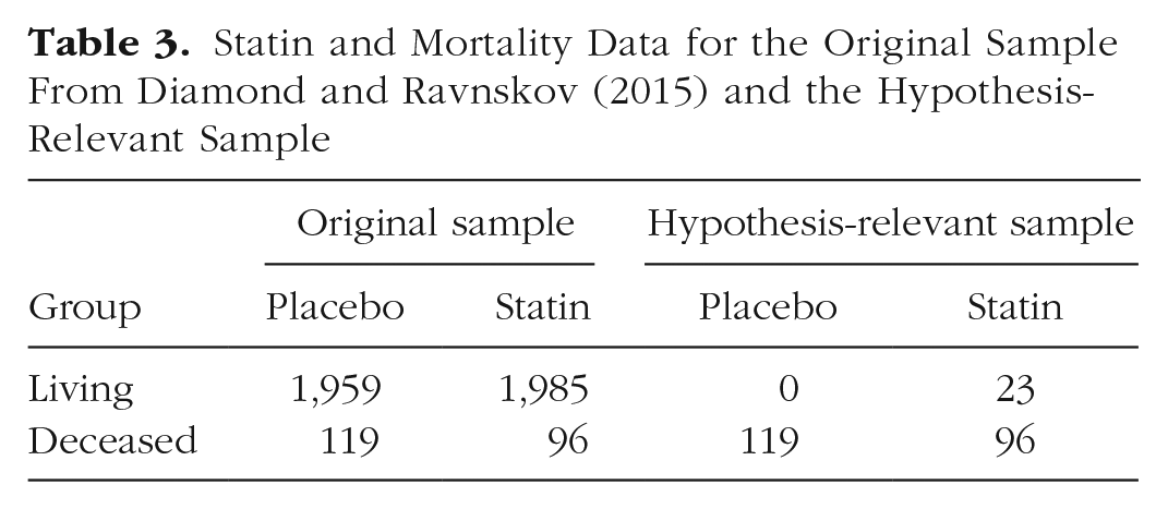
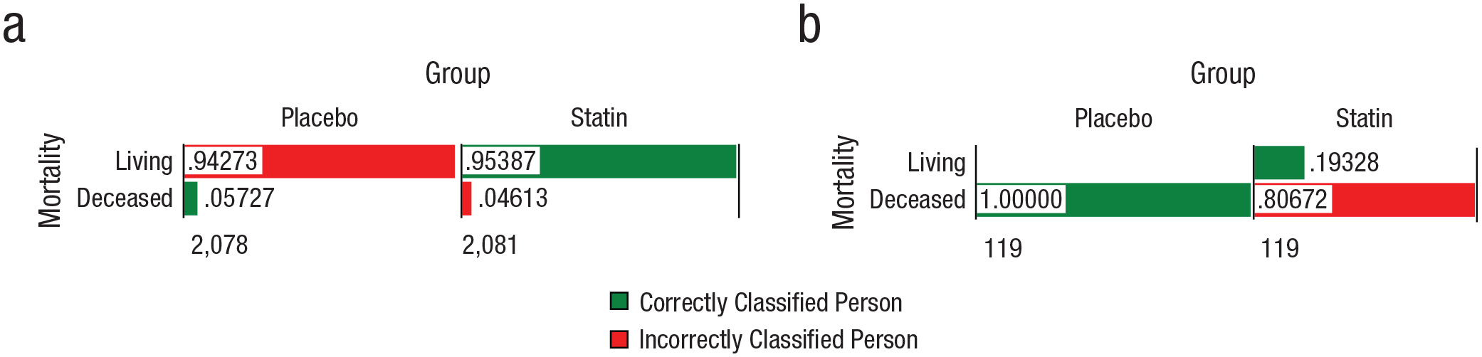
Mortality risk of individuals who received statin treatment or who received placebo (Diamond & Ravnskov, 2015). Results are shown for (a) all 4,159 participants and (b) only hypothesis-relevant participants (n = 238). Conditional proportions are reported in the bars, and column totals are reported below the histograms.

Following Ferguson’s (2009b) reasoning, we computed the hypothesis-relevant frequencies by first determining a base rate using participants who did not take statins and who were deceased at the time of the follow-up (viz., 119/2,078 = .0573). We then applied this base rate to the number of participants who took statins (.0573 × 2,081) and rounded the result to a whole number (119). If statins were ineffective, 119 individuals would be expected to be deceased at the follow-up time. In fact, 96 individuals who took statins were recorded as deceased at the time of the follow-up, which means that 23 hypothesis-relevant individuals were still living. Table 3 reports all of the hypothesis-relevant observations, and a comparison of the two panels of Figure 7 shows a modest increase in the PCC; specifically, the PCC increased from 50.59% in the original sample to 59.66% in the hypothesis-relevant sample. Furthermore, only 19.33% of the hypothesis-relevant individuals in the statin group survived. These results are clearly not as impressive as the results for the Salk vaccine.

Although the PCC offers a unique and apparently conservative metric for judging the effectiveness of an administered drug, the figures are of greatest value. Figures 5, 6, and 7 offer the complete context for traditional effect sizes, such as odds ratios and absolute- and relative-risk-reduction indices, and this context may then reduce errors in their interpretation (see Hoffrage, Lindsey, Hertwig, & Gigerenzer, 2000). For laypersons, pictures are often more effective than numerical or verbal descriptions in conveying the risk associated with a given treatment. Edwards, Elwyn, and Mulley (2002), in fact, recommended using pictures to facilitate communication between professionals and laypersons, and they suggested that “simple bar charts may be preferred over other ‘representations’ (faces, stick figures, etc.)” (p. 830). The cliché that a picture is worth a thousand words seems to apply here.

Conclusion

There are a number of distinct benefits to using the techniques described in this article for treating persons as effect sizes. First, they provide a common metric for conveying the theoretical, practical, or clinical importance of results from various study designs and types of data. The studies discussed employed a mixture of experimental and correlational methods for both discrete and continuous data. Despite this diversity, each set of findings could be described in terms of the number of persons who matched or failed to match expectation.

Second, and perhaps more important, this common metric is one that can be understood by scientists, professionals, and laypersons alike. Although effect-size metrics such as d, r, and η² are more commonly reported by researchers today than 20 years ago, their practical, clinical, or theoretical meanings are often left undiscussed (Ferguson, 2009b; Funder & Ozer, 2019). Instead, their values are routinely labeled as small, medium, or large using common conventions that are divorced from the specific theoretical and methodological contexts of the studies for which they are reported. This state of affairs may reflect a certain inadequacy of many effect-size indices in providing researchers with meaningful statistics (McGraw & Wong, 1992). Person-centered effect sizes, by comparison, may be more easily translated into practically or clinically relevant terms. Policy makers or clinical psychologists studying the efficacy of therapy, for instance, would likely find a statistic like the PCC index to be especially meaningful and useful. Theoretical relevance can likewise be buttressed by person-centered effect sizes; for example, reporting that 80% of the persons in a given study were classified in accordance with expectation provides a commonsense way of conveying the explanatory strength of a theory.

Third, as we showed with each example, computing person-centered effect sizes can reveal patterns in the data that were missed by traditional statistical analyses and effect sizes. Using high-powered computers and incredibly sophisticated statistical models, it is easy to lose touch with one’s data and with the persons in one’s study. The methods presented here encourage the researcher to reconnect with data in a fundamental and theoretically informative manner. Even the process of binning variables forces the researcher to think more carefully about scaling and measurement, as well as distributional assumptions. Doing so paves the way for what is essentially an information gain that goes beyond the PCC indices themselves. Important lessons are learned, and specific avenues for building upon and improving lines of research are opened. In brief, the researcher moves from a mind-set of analyzing data to one of understanding data.

Fourth, person-centered effect sizes are firmly rooted in nonparametric methods that have been developed and investigated alongside parametric methods over the years (S. Siegel, 1956). The ordinal procedure we applied to E. H. Siegel et al.’s (2018) study of affective expressions is an offshoot of the Wilcoxon signed-rank test for dependent observations, and the between-groups comparison method applied to Sawaoka and Monin’s (2018) viral-outrage study is akin to the Mann-Whitney U test (see Ruscio, 2008). In both instances, ties were treated as incorrect classifications, and no attempts were made to derive p values. The graphing procedures used in the remaining examples essentially heeded Tukey’s (1977) well-known call for presenting results in visually compelling ways. The colored and aligned histograms also incorporated results from naive Bayesian classifiers, in accordance with the rising popularity of such methods (see Wasserstein et al., 2019a). Although not strictly identical to traditional nonparametric techniques, then, the PCC index and the procedures demonstrated here are highly familiar to individuals tutored in statistical methods.

Limitations and Further Considerations

The original metrics for the outcome variables in E. H. Siegel et al.’s (2018) affective-suppression study, Sawaoka and Monin’s (2018) viral-outrage study, and Geniole et al.’s (2019) male-aggression study were essentially ignored in computing the person-centered effect sizes. For example, a participant in the affective-suppression study had only to show a decrease in ratings from the positive to the negative condition to be counted as correctly classified for purposes of computing the pairwise PCC index. The magnitude of this decrease was not relevant, nor was the scaling of the ratings themselves. For these types of comparisons, then, the PCC is an effect size that incorporates the underlying ordinal question, “Is one score higher or lower than another?” If one is wedded to a strict parametric analysis or to describing group differences or relationships between variables in the aggregate, this question may be too restrictive, and other indices of effect size, such as Cohen’s d, η², and r_pb, must instead be used (Kirk, 1996; Ruscio, 2008).

With this limitation in mind, there are nonetheless two ways in which magnitudes can be taken into consideration with these person-centered effect sizes. First, traditional statistics can be used in a purely descriptive fashion in conjunction with the PCC index. In E. H. Siegel et al.’s (2018) study on affective suppression, for instance, the 45 participants were separated into three groups: those who fit the expected ordinal pattern (PCC = 24.44%), those whose responses were exactly opposite of expectation, and those who failed to fit the ordinal pattern in some way. Individual magnitudes of change in the ratings across pairs of conditions (positive, neutral, negative) could be computed, examined, and discussed, and basic descriptive statistics such as minimum and maximum values, medians, and standard deviations could be reported for each of the three groups of participants. Second, magnitude can also play a role in the computation of the PCC index itself by using an imprecision value when determining whether a person is classified correctly. Again considering Siegel et al.’s study, a difference of 0.10 on the 5-point rating scale, for example, could be set as the imprecision value. Any participant with an absolute difference in mean ratings less than or equal to 0.10 between pairs of conditions would be counted as incorrectly classified. In this way, small magnitudes that are not theoretically or practically meaningful can be differentiated from larger magnitudes, much as the minimally important difference criterion (Harris & Quade, 1992) for effect sizes is used in power computations, but in this case applied to individuals. Grice, Craig, and Abramson (2015) used such an imprecision value in their study of honeybees’ feeding behavior. Of course, just as is the case in setting the minimally important difference in an effect-size computation, the onus is on the researcher to determine, explain, and defend any imprecision value used to correctly classify observations for the PCC index.

Loss of original variable metrics is also a concern when binning continuous variables, as was done for Geniole et al.’s (2019) study on male aggression. It should be noted that the goal in computing person-centered effect sizes is to engage the data in novel ways and to describe the results of a study in a meaningful or sensible manner (see Funder & Ozer, 2019). In making a decision to bin a variable, “it is the simplicity of the presentation or the facilitation of communication of results, rather than the simplicity of data analysis, that is the guiding principle” (Vargha et al., 1996, p. 280). Nonetheless, as in analyses of median-split (dichotomized) variables, individuals with scores close to the cut points are treated as essentially the same as those with scores close to the variable’s extremes. Such binning may result in the loss of important information (viz., magnitude differences between persons), as has been discussed in cautionary work regarding dichotomization of variables in the computation of the binomial effect-size display (Hsu, 2004). This valid concern should compel researchers to pay close attention to variables’ distribution and to display them when possible. Blindly conducting a simple median split of the behavioral-aggression scores in Geniole et al.’s study in order to compute a binomial effect-size display or PCC , for instance, would have ignored the fact that a relatively large proportion of men scored zero on the measure. This distinctive feature of the data was evident in the histogram and was subsequently taken into account in the analysis. Dividing the behavioral-aggression scores into three groups also showed that the computation of the PCC is not restricted to dichotomous groups. Any quantitative variable can be binned into different numbers of groups, so that researchers can examine more complex patterns and assess the impact of differing cut points. Multiple bins might also correspond to theoretically or practically meaningful groups, such as people with minimal, mild, moderate, and severe depression, as identified by scores on a depression scale.

Employing different binning strategies and setting imprecision values in a study will rightly raise important concerns about investigator bias. A researcher who analyzes a sample of data with several sets of bins, for instance, and then reports only the result yielding the highest and most impressive PCC index is engaging in behavior that is fundamentally no different from p-hacking (Simmons, Nelson, & Simonshohn, 2011). The reported result will not likely lead to a valid interpretation of the findings, nor will it likely be replicated in future studies. One must therefore keep in mind that the methods discussed in this article are part of a larger process of collecting, analyzing, and interpreting data in which “researchers have many decisions to make: Should more data be collected? Should some observations be excluded? Which conditions should be combined and which ones compared? Which control variables should be considered? Should specific measures be combined or transformed or both?” (Simmons et al., 2011, p. 1359). These decisions must be made and reported with complete transparency, and the results of all analyses must be presented in the final published report or in supplementary material in accord with the principles of OSF. Perhaps ideally, methods for computing PCC indices for a given study, including decisions regarding binning or imprecision values, can be preregistered as part of the study design and planned statistical analyses as a means for controlling investigator bias (van ’t Veer & Giner-Sorolla, 2016).

Finally, we presented person-centered effect sizes to answer the general question, “How many people in my study behaved or responded in a manner consistent with theoretical expectation?” The goal was to describe the samples, not to draw inferences about the populations from which they were nonrandomly drawn. More generally, the goal of this article was to show how person-centered effect sizes can be computed and interpreted across a range of study designs. Nonetheless, the question of generalizing beyond a given sample can be considered in the realm of effect sizes. Ruscio (2008), for instance, has shown that a person-centered effect size referred to as A yields unbiased estimates of population parameters and stable standard errors across normal and nonnormal distributions. A is similar to the PCC index computed for Sawaoka and Monin’s (2018) study, in which each person in the viral condition was compared with every other person in the nonviral condition. With A, however, ties are not treated as strict misclassifications (Delaney & Vargha, 2002). ²

Cota (2017) showed that with two- and three-group between-participants designs and binned dependent variables, sample estimates of the PCC were unbiased with sample sizes of at least 100. Similarly, Valentine, Buchanan, Scofield, and Beauchamp (2019) showed that for a repeated measures design, such as in E. H. Siegel et al.’s (2018) study, the PCC index yielded stable estimates with large sample sizes. It is important to point out, however, that simulation studies of effect sizes routinely entail random sampling, which is a condition rarely met in practice. Most researchers work with convenience samples, and Sauer (2018) has shown that under such circumstances, the robustness of the PCC for a given study may be assessed using a randomization test. Investigating and elucidating the inferential properties of any statistic is clearly a complex and sophisticated process, and further work on person-centered effect sizes (e.g., see Ruscio & Mullen, 2012), such as the PCC, is needed. Such work will lead to a greater understanding of these effect sizes, which will then improve their efficacy as tools for identifying and explaining patterns within samples of observations.