Sage Journals: Discover world-class research

Abstract

Many statistical scenarios initially involve several candidate models that describe the data-generating process. Analysis often proceeds by first selecting the best model according to some criterion and then learning about the parameters of this selected model. Crucially, however, in this approach the parameter estimates are conditioned on the selected model, and any uncertainty about the model-selection process is ignored. An alternative is to learn the parameters for all candidate models and then combine the estimates according to the posterior probabilities of the associated models. This approach is known as Bayesian model averaging (BMA). BMA has several important advantages over all-or-none selection methods, but has been used only sparingly in the social sciences. In this conceptual introduction, we explain the principles of BMA, describe its advantages over all-or-none model selection, and showcase its utility in three examples: analysis of covariance, meta-analysis, and network analysis.

Keywords

model comparison Bayesian analyses ANCOVA meta-analysis network analysis uncertainty Bayesian model averaging open materials

Imagine waiting at a railway station for a train that is supposed to take you to an important meeting. The train is running a few minutes late, and you start to deliberate about whether or not to use an alternative mode of transportation. In your deliberation, you contemplate the different scenarios that could have transpired to cause the delay. There may have been a serious accident, which means your train will be delayed by several hours. Or perhaps your train has been delayed by a hailstorm and is likely to arrive in the next half hour or so. Alternatively, your train could have been stuck behind a slightly slower freight train, which means that it could arrive at any moment. In your mind, each scenario i corresponds to a model of the world H_i that is associated with a different distribution of estimated delay t, denoted p(t|H_i). You do not know the true scenario, H′, but you do not really care about it either; in your hurry, all that is relevant for your decision to continue waiting or to take action is the (distribution of the) delay p(t) unconditional on any particular model H_i.

In probabilistic terms, p(t) is referred to as the Bayesian-model-averaging (BMA) estimate (see, e.g., Jeffreys, 1939, p. 296, or Jevons, 1874, p. 292). Rather than first selecting the single most plausible scenario $\hat{H}$ and then using p(t| $\hat{H}$ ) for all decisions and conclusions, BMA provides an assessment of the delay t that takes into account all scenarios simultaneously. This is accomplished by computing a weighted average, with weights that indicate the plausibility of each scenario. For instance, although it is in principle possible that the railway company has decided to start major construction work today, thus causing a delay of weeks, most likely you would have learned about this sooner. Therefore, the prior model plausibility p(H_i) (before you observe anything) of this scenario is low, and its implied long delay contributes only little to p(t). More formally, the BMA estimate is obtained through the equation $p (t) = \sum_{i} p (t H_{i}) p (H_{i})$ . The BMA estimate is adjusted as new information becomes available; for instance, your beliefs will be updated by railway-station announcements, time passing without the train arriving, and the increasingly agitated faces of your fellow travelers. This information can be referred to collectively as “data,” and the BMA estimate becomes $p (t data) = \sum_{i} p (t H_{i}, data) p (H_{i} data)$ . Thus, your observations influence not only the predicted time for each scenario, but also the probability of the scenarios themselves. The resulting distribution p(t|data) represents your beliefs about the delay, after having made observations, while simultaneously taking all models into account.

The model-averaged estimate of the delay time, p(t|data), respects the uncertainty about the possible scenarios that might explain the delay. This formulation provides a more nuanced and prudent estimate than if you had simply assumed the most plausible scenario to be true. For instance, suppose that p(H_accident) = .15, p(H_hailstorm) = .25, and p(H_{freight train}) = .60. You could base your estimate of the delay time solely on the most probable scenario, H_{freight train}, but this would open you up to a substantial probability (.15 + .25 = .40) of mistaking the scenario and its corresponding delay.

Despite the intuitive application of BMA in examples from daily life, it is severely underutilized in the social-sciences literature (for noteworthy exceptions, see Gronau et al., 2017; Kaplan & Lee, 2018; for recommendations and guidelines, see Appelbaum et al., 2018), even though it is regularly employed in other disciplines (see Fragoso, Bertoli, & Louzada, 2018, for a review; see Steel, in press, for a survey on BMA in economics). This mismatch suggests that researchers in the social sciences remain unaware of the advantages of adopting Bayesian statistics (Vandekerckhove, Rouder, & Kruschke, 2018) or do not have access to easy-to-use software that implements BMA and other Bayesian methods. With this introductory article, we hope to increase awareness of the principles behind BMA and of the availability of tools that make BMA straightforward to apply. We start out by explaining the key concepts involved. Subsequently, we demonstrate the use of BMA in three concrete examples (analysis of covariance, or ANCOVA; meta-analysis; and network analysis) to showcase the distinct advantages that BMA has over the select-a-single-model approach.

Bayesian Model Averaging and Its Advantages

In this section, we provide an informal exposition of BMA. The appendix provides more exact definitions of the relevant concepts, but these are not required to understand the examples and discussion here. Box 1 provides a quick reference of the informal definitions we introduce in this section.

Box 1.

Glossary of Terms Used in Bayesian Model Averaging

Prior distribution: Initial beliefs about the relative plausibility of parameter values, before the data have been seen.

Likelihood: The probabilistic prediction assigned to the observed data under a specific parameter value.

Posterior distribution: Updated beliefs about the relative plausibility of parameter values, after the data have been seen.

Model: The data-generating process that is hypothesized to account for a phenomenon of interest. Prior and posterior model probability: Initial and updated beliefs about the plausibility of a model, respectively.

Prior and posterior model odds: The ratio of the prior model probabilities of two models and the ratio of the posterior model probabilities of two models, respectively.

Bayes factor: The change from prior to posterior model odds brought about by the data; equivalently, how much more likely the observed data are under one model versus another.

Bayesian model average: A parameter estimate (or a prediction of new observations) obtained by averaging the estimates (or predictions) of the different models under consideration, each weighted by its model probability.

Posterior inclusion probability: The model-averaged probability of including a certain predictor in the model, given the observations; an indicator of how relevant a predictor is across all possible models.

Inclusion Bayes factor: The change from prior to posterior inclusion odds, which are defined analogously to the prior and posterior model odds.

In a statistical analysis, one is typically interested in inference or prediction of some unknown quantity θ. Bayes rule prescribes how observed data update prior beliefs for θ (i.e., p(θ)) to posterior beliefs (i.e., p(θ|data)). However, just as in the introductory example, it is often the case that there exist multiple hypotheses or models H_i that describe the relationship between θ and the data. Bayes rule can be used once more for models,¹ to compute the posterior model probability (PMP), that is, p(H_i|data), which describes the plausibility of H_i after the data are observed. The PMP can be used to identify the most plausible model, given the data, an activity referred to as model selection (Burnham & Anderson, 2004).

When a single model dominates the distribution of PMP, it is sensible to use this particular model as one’s best guess of the true situation. One may then compute, for example, the probability of θ in light of the data, given this dominating model. Often however, there is remaining uncertainty not only about parameters, but also about the underlying true model. In this case, a Bayesian analysis allows one to take into account not only uncertainty about the parameters given a particular model, but also uncertainty across all models combined. This is done via BMA, in which one takes the combined distribution of a parameter, weighted by the PMP of all candidate models (Draper, 1995; Jeffreys, 1939; Jevons, 1874; Madigan, Raftery, York, Bradshaw, & Almond, 1994).

The intuition underlying BMA is illustrated by the BMA pandemonium in Figure 1.² This cartoon illustrates the following BMA concepts. Each candidate model is represented by a single demon; together, this legion of demons represents the collection of possible models. Each demon shouts its beliefs about parameters, which reflect how the corresponding model assumes that parameters are distributed. The demons’ sizes reflect the model probabilities, that is, how plausible each model is before one has observed any data. A priori, the models are deemed equally likely; that is, the demons are all the same size. Once the models are presented with observations—as the demons are presented their sustenance—the probabilities of the models change; models consistent with the data become more probable (i.e., the associated demons grow in size), whereas models that are relatively inconsistent with the data become less probable (i.e., the associated demons shrink). From a Bayesian perspective, no demon ever completely vanishes,³ and thus no demon completely dominates the pandemonium, just as no model is ever without a doubt the “true” model.

Fig. 1.

A pandemonium interpretation of Bayesian model averaging. Each model is represented by a demon, which shouts its beliefs about its model parameters. In the top panel, the demons’ sizes, and hence shouting volume, are given by the model prior. In the middle panel, the demons are confronted with data; they grow if they predicted the data relatively well and shrink if they predicted the data relatively poorly. The bottom panel shows the demons’ sizes after they gorge on the data. In making the final inference about the parameters of interest, it is prudent to be informed by all the demons (weighted by their importance), not just the demon that is largest. Concept by the authors, artwork by Viktor Beekman; available under a CC-BY license at BayesianSpectacles.org/library/.

Each demon shouts its own prediction (such as a train delay), which represents one’s beliefs about parameters conditioned on that demon. If one demon completely dominates the posterior model distribution (i.e., one demon is much larger than any of the others, after having seen the data), it shouts much louder than any of the alternatives. The average prediction is therefore dominated by this demon’s claim, in which case it would be appropriate to select this single demon for inference. In practice, however, much uncertainty usually remains in the posterior model distribution; this uncertainty is reflected by the presence of many demons that are roughly equally small. In this situation, the optimal prediction is obtained by averaging over the demons’ cacophony, rather than listening only to the arbitrarily slightly largest demon.

BMA fundamentally starts with uncertainty across models, and then Bayesian updating of beliefs is applied according to observations. Compared with single-model selection, the BMA framework offers a number of advantages:

BMA reduces the overconfidence (i.e., underestimated uncertainty) that emerges when model uncertainty is ignored. If one proceeds with a single selected model $\hat{H}$ , one has essentially made the claim that p( $\hat{H}$ |data) = 1. Naturally, this never occurs except in simulations. Analyses based on BMA respect the uncertainty about the models.

BMA results in optimal predictions under several loss functions, such as the logarithmic or the squared error loss (Hoeting, Madigan, Raftery, & Volinsky, 1999). This may seem counterintuitive; after all, surely the optimal predictions come from using the true model instead of a weighted average. However, as the previous point indicates, there is no way to consistently identify the correct model. The error that this induces is mitigated by BMA.

BMA avoids the all-or-nothing mentality that is associated with classical hypothesis testing, in which a model is either accepted or rejected wholesale. In contrast, BMA retains all model uncertainty until the final inference stage, which may or may not feature a discrete decision.

Procedures based on the selection of a single best model may yield sudden changes in estimates when the observation of new data, or the repetition of an experiment, leads to the selection of a different best model. Even the addition of a single observation can cause a sudden discrete shift in the estimates. BMA instead gracefully updates estimates as the data accumulate, and the resulting model weights are continually adjusted. This way, the variance of parameter estimates across experiments is reduced, at the cost of assigning nonzero probability to some “wrong” models. A related problem with selecting a single best model is that the observation of new data may require the resuscitation of a model that was previously rejected, which seems incoherent.

BMA is relatively robust to model misspecification. If one does select a single model, then one had better be sure of being correct. With BMA, a range of rival models contribute to estimates and predictions, and chances are that one of the models in the set is at least approximately correct.

BMA is particularly useful when the goal is prediction or parameter estimation but multiple competing models remain viable a posteriori. In this context, the models are a nuisance factor; they are not of direct interest, but nonetheless they influence prediction and estimation. Given the posterior beliefs about the candidate models, BMA eliminates this nuisance factor to produce the best predictions or parameter estimates. BMA is less useful when a single model dominates all others, or when the goal is to quantify evidence for a set of candidate models. For instance, each candidate model may represent a different theory of a physical process, and one may wish to identify the model that receives the most support. In this setting, the models are not a nuisance factor; they are the focus of the analysis. It should furthermore be noted that when BMA is used to produce model-averaged point estimates, the results may not be representative for any of the competing models; for instance, suppose that model A has most posterior mass near 0 and model B has most posterior mass near 1; the BMA point estimate may be near 0.5, a value that is unlikely under either model. However, the fault here is not with BMA, but with the attempt to summarize a multimodal posterior distribution by a single point. Note that, in terms of quadratic loss, the point estimate remains the optimal choice (Zellner & Siow, 1980, pp. 600–601).

The main challenge of BMA, and one that is often glossed over, is arguably that the results depend on the prior probabilities that are assigned to the candidate models. The common choice is to assume that all candidate models are equally likely a priori, but different approaches are possible and will affect the results. For instance, one may decide to assign less prior weight to models with many parameters than to models with few parameters (Consonni, Fouskakis, Liseo, & Ntzoufras, 2018; Wilson, Iversen, Clyde, Schmidler, & Schildkraut, 2010). As is usually the case in Bayesian inference, one may specify different prior model probabilities and examine the degree to which the BMA results are qualitatively robust to changes in the prior.

Next, we provide three examples of how BMA can be used advantageously in statistical scenarios relevant for psychology: ANCOVA designs, meta-analysis, and network analysis. These examples are intended as illustrations of how BMA can be used to provide the researcher with more robust and nuanced results. The specific modeling choices that are used, such as the prior distributions on model parameters, are shown for completeness but may safely be ignored by readers who are primarily interested in the key concepts. For more background information on the specific analyses, we refer to the work cited in connection with each of the examples.

Disclosures

All materials used for the analyses in this article are available on the Open Science Framework, at https://osf.io/dbsuz/.

Example 1: Bayesian Model Averaging for ANCOVA Designs

ANCOVA is one of the canonical statistical analysis techniques in psychology. It also demonstrates nicely an important application of BMA. In regression frameworks such as ANCOVA, models are constructed by selecting predictors from an existing set of variables. If a predictor can be either included or excluded, then for a set of k predictors, there are 2^k possible models. This means that a moderately large set of predictors will spawn a very large model space that is unlikely to be dominated by any single model. How, then, should one evaluate the support that the data provide for the importance of any specific predictor? In BMA, the answer is to compute for each predictor an inclusion probability. This inclusion probability is the sum of the PMPs over models that included this particular predictor.

Here we illustrate such a BMA approach to ANCOVA (Rouder, Engelhardt, McCabe, & Morey, 2016; Rouder, Morey, Speckman, & Province, 2012; Rouder, Morey, Verhagen, Swagman, & Wagenmakers, 2017), using data from Shen, Yang, Zhang, and Zhang (2018).⁴ Shen et al. investigated the effect of expressive writing on Test Anxiety Scale (TAS) scores. Each of 75 high-school students was assigned randomly to either an expressive-writing condition or a control condition. For 30 days, the students engaged daily in expressive writing about positive emotions (the expressive-writing group) or were asked to write down their daily events (the control group). The TAS was administered before and after the intervention. In total, the data set contains four variables of interest: gender, group (treatment condition), the TAS score on the pretest, and the dependent variable, the TAS score on the posttest. The condition means for the pretest and posttest are shown in Figure 2. The ANCOVA analyses used the default prior distributions (i.e., the Jeffrey-Zellner-Siow prior setup for the fixed effects with a scale parameter of 0.5; Clyde, Ghosh, & Littman, 2011; Jeffreys, 1939; Rouder, 2012; Zellner & Siow, 1980).

Fig. 2.

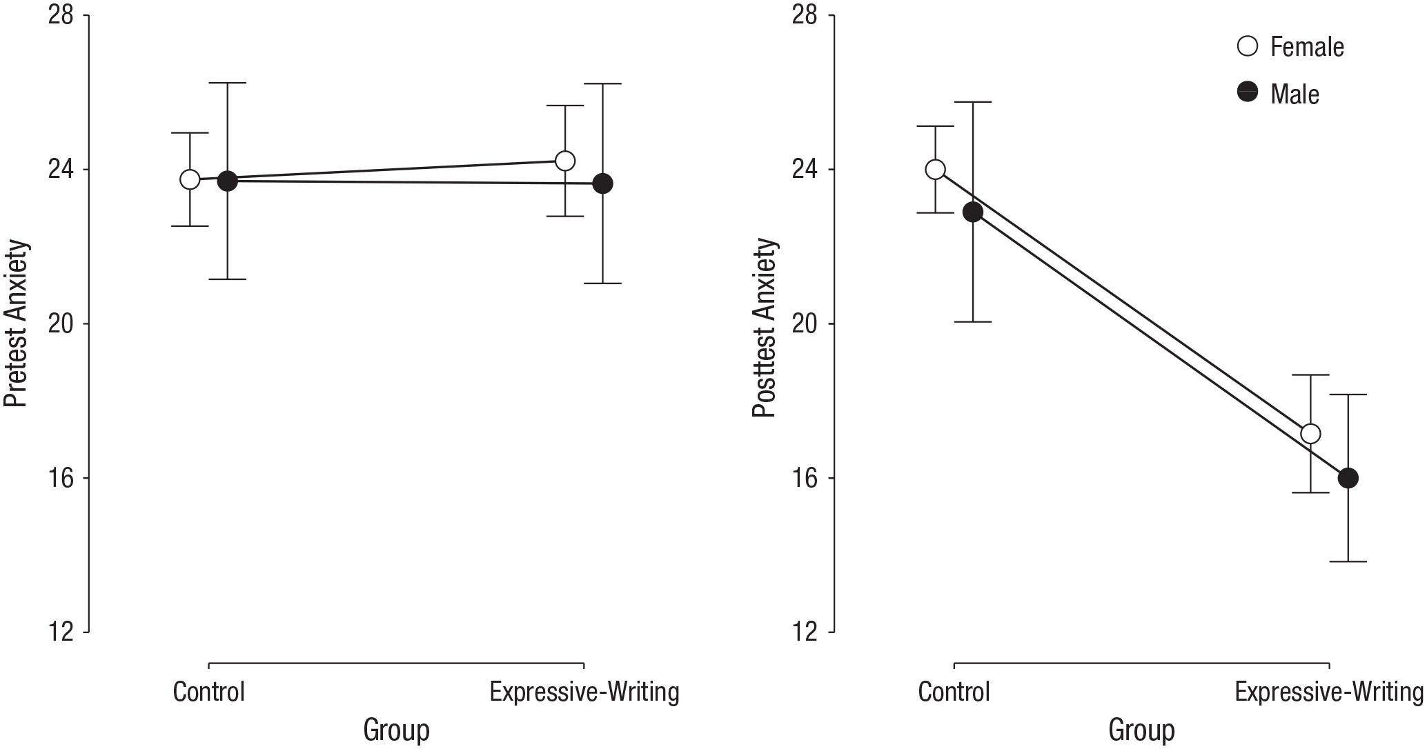
Mean Test Anxiety Scale scores on the pretest (left panel) and posttest (right panel) in Shen, Yang, Zhang, and Zhang’s (2018) data. Results are shown separately for males and females in the control group and the expressive-writing group. A lower score indicates that a student was less anxious about taking tests. Error bars signify 95% credible intervals.

The different models to test correspond to the inclusion of any number of these predictors, as well as the interaction effect between group and gender; these are all compared with the null model. This results in 10 models (9 alternatives + 1 null), whose PMPs, p(H|data), are listed in Table 1. This table also displays Bayes factors (BFs), which are the natural Bayesian way of quantifying the result of model comparison. Mathematically, BF₁₀ is the ratio of the probability of the data under H₁ over the the probability of the data under H₀; that is, BF₁₀ = p(data|H₁)/p(data|H₀). Intuitively, the Bayes factor describes how much more likely the data are under one model compared with another. For instance, a BF₁₀ of 5 means that the data are 5 times more probable under the alternative model, H₁, compared with the null model, H₀. Table 1 shows the values of BF_tj, which is the Bayes factor that compares the most likely model after the data are seen, H_t, with the jth model, H_j.

Table 1.

Model Comparison for the Bayesian Analysis of Covariance on the Data of Shen, Yang, Zhang, and Zhang (2018)

Model	p(H)	p(H\|data)	BF_tj
Pretest + gender + group	.1	.445	1.000
Pretest + group	.1	.395	1.125
Pretest + gender + group + Gender * Group	.1	.160	2.781
Group	.1	2.439 × 10⁻⁷	1.823 × 10⁶
Gender + group	.1	1.201 × 10⁻⁷	3.702 × 10⁶
Gender + group + Gender * Group	.1	4.126 × 10⁻⁸	1.078 × 10⁷
Pretest	.1	8.795 × 10⁻¹⁷	5.056 × 10¹⁵
Pretest + gender	.1	4.150 × 10⁻¹⁷	1.072 × 10¹⁶
Null model	.1	3.412 × 10⁻¹⁷	1.303 × 10¹⁶
Gender	.1	1.392 × 10⁻¹⁷	3.195 × 10¹⁶

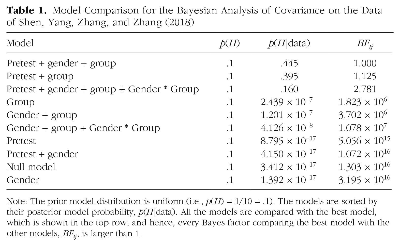
Note: The prior model distribution is uniform (i.e., p(H) = 1/10 = .1). The models are sorted by their posterior model probability, p(H|data). All the models are compared with the best model, which is shown in the top row, and hence, every Bayes factor comparing the best model with the other models, BFtj, is larger than 1.

Table 1 reveals that the top three models are much better supported by the data than the other models, as they have much higher evidence. Also, the Bayes factors of the top model compared with the second and third models are relatively low, whereas the Bayes factors of the top model compared with the remaining models are enormous. Among these top three models, however, there is no clear winner. Specifically, there is substantial uncertainty about whether adding gender and the interaction between gender and group explains the data better.

In this example, we have a limited number of predictors, and hence a limited number of different models. As the table shows, it is possible to exhaustively enumerate all models and their probabilities, which allows a fully informed and nuanced interpretation of this analysis. However, for data sets with more predictors, such a table becomes much too large to interpret. In that case, one can summarize the results using the Bayesian model average, in particular, the inclusion probabilities of the individual predictors. We have done so for the current example in Table 2. Both pretest and group definitely improve the predictive performance of the model; their posterior inclusion probabilities are approximately 1, and the Bayes factors of models with these predictors versus models without these predictors (also shown in Table 2) are huge. However, there is a lot of uncertainty about whether to include gender and the interaction between gender and group. In stark contrast, the model with the highest posterior probability includes the predictor pretest, group, and gender. The correct conclusion is therefore that pretest score and condition explain posttest score, but that the data are not informative enough to draw conclusions about gender and the interaction between gender and group.⁵

Table 2.

Inclusion Probabilities and Bayes Factors for the Predictors in the Bayesian Analysis of Covariance on the Data of Shen, Yang, Zhang, and Zhang (2018)

Effect	p(incl)	p(incl\|data)	BF _inclusion
Pretest	.500	1.000	2.483 × 10⁶
Group	.600	1.000	6.005 × 10¹⁵
Gender	.600	.611	1.047
Gender * Group	.200	.164	0.783

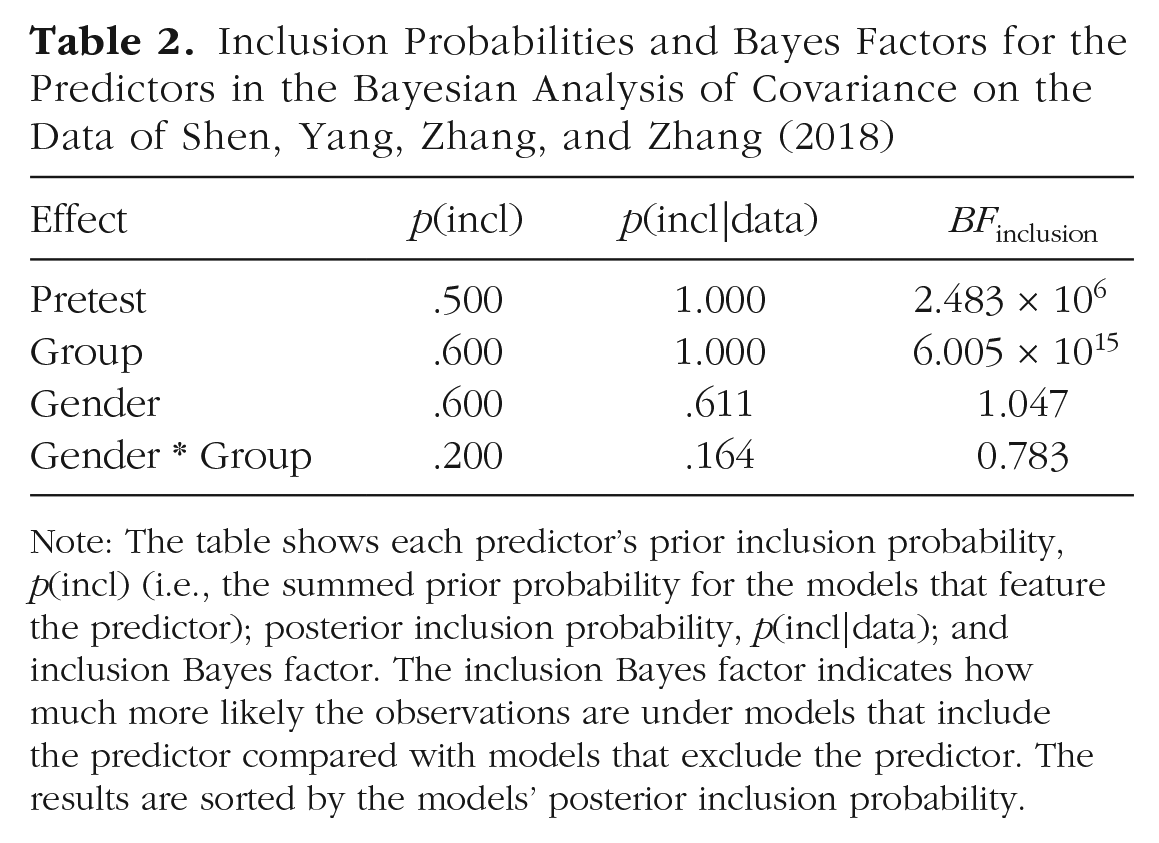
Note: The table shows each predictor’s prior inclusion probability, p(incl) (i.e., the summed prior probability for the models that feature the predictor); posterior inclusion probability, p(incl|data); and inclusion Bayes factor. The inclusion Bayes factor indicates how much more likely the observations are under models that include the predictor compared with models that exclude the predictor. The results are sorted by the models’ posterior inclusion probability.

Example 2: Bayesian Model Averaging in Meta-Analysis

Meta-analysis is the joint analysis of multiple studies on the same topic. As meta-analysis effectively combines the samples from all the studies, its statistical power usually is much greater than that of the individual studies, which makes it easier to detect an effect (δ ≠ 0) and estimate its size (Cooper, Hedges, & Valentine, 2009; Schmidt, 1992). However, the way in which different studies should be combined is often not immediately obvious. A common dilemma in meta-analysis is whether the study replications share a particular effect size (i.e., the between-study variance is zero, τ = 0), or whether there exists between-study effect-size heterogeneity (i.e., τ ≠ 0; Gronau et al., 2017). Instead of assuming one or the other, the researcher may perform meta-analysis using BMA. In this case, the analysis yields an estimate of the group mean effect size, regardless of one dominant model; the researcher computes the PMP of each model and subsequently the weighted average of the effect size across the models. The four candidate models are as follows:

H₀ (fixed effect): δ = 0, τ = 0;

H₁ (fixed effect): δ ≠ 0, τ = 0;

H₀ (random effect): δ = 0, τ ≠ 0; and

H₁ (random effect): δ ≠ 0, τ ≠ 0.

As an example, we consider a meta-analysis of the facial feedback hypothesis (e.g., Strack, Martin, & Stepper, 1988), which states that people’s affective responses may be guided in part by their facial expressions. Specifically, Strack et al. (1988) argued that people judge cartoons to be more amusing when they hold a pen between their teeth (which induces a smile) than when they hold a pen with their lips (which induces a pout). The original study found a rating difference of 0.82 on a 10-point Likert scale, which was interpreted as support for the hypothesis. In a recent replication project, researchers at 17 independent labs attempted to replicate the effect using a preregistered study protocol (Wagenmakers et al., 2016). Here we analyze these studies using a BMA meta-analysis (e.g., Gronau et al., 2017; Scheibehenne, Gronau, Jamil, & Wagenmakers, 2017; for an R implementation, see the metaBMA package—Heck, Gronau, & Wagenmakers, 2019). For the between-study effect-size heterogeneity (τ) we use an inverse-gamma(1.0, 0.15) prior distribution, which captures a reasonable range of possible heterogeneities (see Gronau et al., 2017, for a more detailed motivation for this prior). For the effect size (δ) itself, we consider two different possible priors. The first has become a default choice in psychology and is a zero-centered Cauchy( $1 / 2 \sqrt{2}$ ) distribution (Morey & Rouder, 2015). The second is the Oosterwijk prior, which is an informed prior that was elicited from Suzanne Oosterwijk, a social psychologist at the University of Amsterdam (Gronau et al., 2017; Gronau, Ly, & Wagenmakers, 2020). It is implemented as a t distribution with location 0.350, scale 0.102, and 3 degrees of freedom. Compared with the default prior, this distribution places more mass on small-to-medium effects.

In Figure 3, we show the model-comparison results for each of the 17 individual replications, as well as the overall results for the different models used in the meta-analysis. Each panel shows the distribution of the estimated effect size, as well as the Bayes factors that compare the null model with the alternative. Regardless of the specific prior distribution (which we do not discuss in detail here), the evidence in favor of the null hypothesis is compelling. That is, the data are approximately 15 times more likely under the absence of a facial feedback effect given the default prior and approximately 55 times more likely under the absence of a facial feedback effect given the informed prior. The PMPs are shown in Table 3. Regardless of the effect-size prior (i.e., default or informed), the models that include an effect are relatively implausible.

Table 3.

Posterior Model Probabilities for the Meta-Analysis of the 17 Facial Feedback Studies in Wagenmakers et al.’s (2016) Registered Replication Report

Model	p(H)	p(H\|data)
Model	p(H)	Default prior	Informed prior
H₀ (fixed effect): δ = 0, τ = 0	.25	.802	.841
H₁ (fixed effect): δ ≠ 0, τ = 0	.25	.054	.015
H₀ (random effect): δ = 0, τ ≠ 0	.25	.135	.141
H₁ (random effect): δ ≠ 0, τ ≠ 0	.25	.009	.003

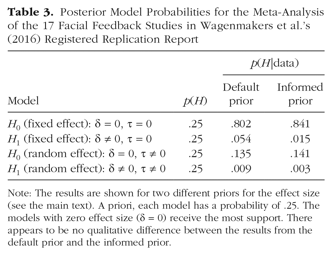
Note: The results are shown for two different priors for the effect size (see the main text). A priori, each model has a probability of .25. The models with zero effect size (δ = 0) receive the most support. There appears to be no qualitative difference between the results from the default prior and the informed prior.

Fig. 3.

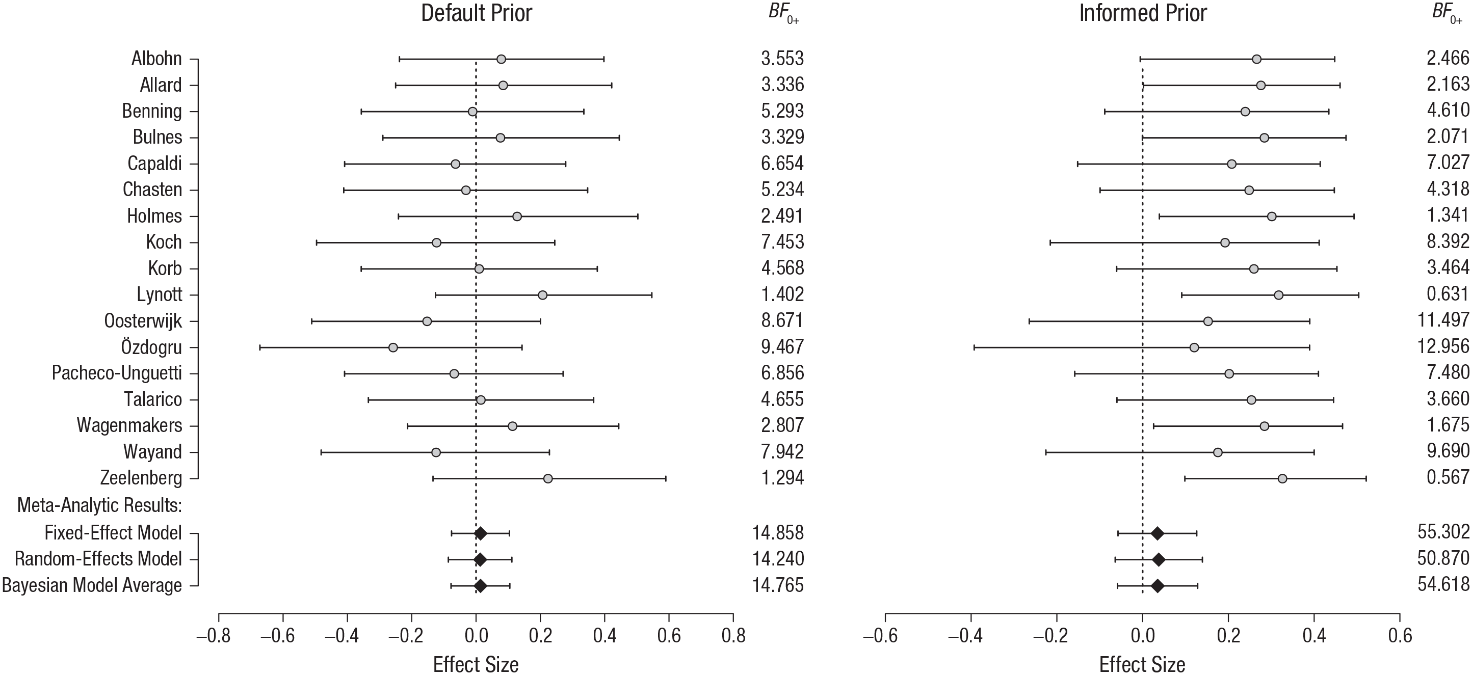
Results of the 17 facial feedback studies in the Registered Replication Report by Wagenmakers et al. (2016). Results are shown for two different prior distributions: a default prior and an informed prior (see the main text). Shown are the 95% highest-density intervals (horizontal bars) and the medians (circles) of the posterior distributions of effect sizes, given δ ≠ 0. In addition, the Bayes factors, BF₀₊, indicate the strength of evidence for the null hypothesis, H₀, relative to the alternative, H₁, that is, how much more likely the data are under the absence than under the presence of an effect. For instance, the Zeelenberg experiment yielded a BF₀₊ of 1.294 under the default prior, indicating only a smidgen of evidence for the absence of an effect. The bottom three rows indicate the estimated effect size obtained via the meta-analysis models with a fixed effect and with random effects, and the Bayesian model average of the two. The figure shows that most individual studies provided only weak evidence for the absence of an effect. Bayesian-model-averaged meta-analysis averages over both the models with zero effect size and those with nonzero effect size and provides much more compelling evidence than the individual studies do.

If we were to predict the outcome of a new experiment testing the facial feedback hypothesis, we would need to average the predictions of all four of these models, weighted by these posterior probabilities. Because the null models are clearly more probable than the alternative models, the resulting BMA prediction would be that there is little effect.

Example 3: Bayesian Model Averaging in Network Analysis

Network analysis is an increasingly important tool in psychometrics (Epskamp, Rhemtulla, & Borsboom, 2017; Marsman et al., 2018; van der Maas, Kan, Marsman, & Stevenson, 2017), as well as in cognitive neuroscience (Petersen & Sporns, 2015; Smith et al., 2011). In such analyses, the interactions among a large number of variables are modeled as a network; the weight of each connection is typically given by the partial correlation between its variables (and set to zero if there is no interaction according to the network). Even though network analysis is becoming increasingly popular, it also brings a number of interesting new challenges, such as how to present its results in an interpretable way and how to properly deal with uncertainty in network estimation. In this section, we demonstrate how BMA addresses both of these issues.

In the context of network analysis, a model H represents a particular configuration of present/absent connections between variables (the presence or absence of a connection is similar to the presence or absence of a predictor in the ANCOVA example). As we noted earlier, in regression models, the number of models is 2^k for k predictors, which makes it difficult to enumerate all candidate models. This problem is much worse in network analysis, in which the number of models grows as 2^k(k−1)/2, for k network variables. Needless to say, it is impossible to exhaustively enumerate all models even for small k.⁶

In realistic applications, it is exceedingly unlikely that one model completely dominates the posterior model distribution. Instead, many models (that perhaps differ pairwise by only a few connections) will be roughly equally probable. BMA is well suited to obtain an appropriate estimate of which connections are present and which are not, and what the weights of these connections are (Hinne, Janssen, Heskes, & van Gerven, 2015; Penny et al., 2010). We demonstrate what BMA can offer to network analysis using a data set containing answers to the Big Five personality inventory (Goldberg, 1999; Revelle, Wilt, & Rosenthal, 2010), which measures personality features relating to openness to experience, conscientiousness, extraversion, agreeableness and neuroticism. In the corresponding network, a connection represents conditional depencence between the personality traits, and the weight of this connection represents the partial correlation between the traits.

The BDgraph R package is used for BMA network analysis (Mohammadi & Dobra, 2017). We use a uniform prior on the network structure and a G-Wishart(d,D) prior distribution on the partial correlations. This distribution allows one to learn connection weights only for those connections that are present in H_i. Its arguments are the degrees of freedom, d, which we set to 3, and the scale matrix, D, which represents the expected partial-correlation structure. Here, we set D to the p × p identity matrix, which represents that a priori we have no reason to believe that any connection has a particular nonzero weight. This amounts to a vague and proper prior (Moghaddam, Khan, Murphy, & Marlin, 2009; Roverato, 2002).

Note that it becomes impractical to visualize the BMA distribution for every connection in a network. We therefore summarize the BMA distribution by its expectation. Although information is lost, this approach allows us to succinctly summarize the distributions over networks and corresponding weights.

Table 4 lists the probabilities of the data under the 10 most likely models. As expected, the differences among the top models are negligible. For instance, the data are only 1.31 times more likely under the top model compared with the 2nd-best model, and only 1.79 times more likely under the top model compared with the 10th-best model. This shows that there is strong uncertainty about which model best describes the data. Typical network analyses neglect this information and indicate only what is the most likely model, but clearly, summarizing the analysis by selecting only the most likely model does not do justice to the uncertainty that these data imply. In terms of the BMA pandemonium analogy of Figure 1, the demon representing the top model increased substantially in size (relative to its minuscule size in the prior) after feasting on the observations. However, its PMP is still only .00558, a tiny fraction compared with the total mass of all the demons (which is 1, by definition). This once more illustrates the imprudence of selecting a single most probable model, which is warranted only when the demon’s PMP approaches 1.

Table 4.

Bayesian Model Comparison for the Top-10 Network Structures in Example 3

Model rank	p(H\|data)	BF_tj
1	5.58 × 10⁻³	1.00
2	4.23 × 10⁻³	1.31
3	4.17 × 10⁻³	1.34
4	4.08 × 10⁻³	1.37
5	3.58 × 10⁻³	1.56
6	3.51 × 10⁻³	1.59
7	3.49 × 10⁻³	1.60
8	3.43 × 10⁻³	1.62
9	3.31 × 10⁻³	1.68
10	3.11 × 10⁻³	1.79

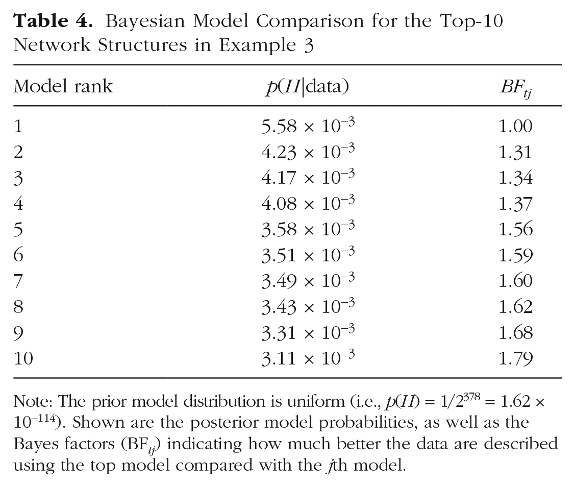
Note: The prior model distribution is uniform (i.e., p(H) = 1/2³⁷⁸ = 1.62 × 10⁻¹¹⁴). Shown are the posterior model probabilities, as well as the Bayes factors (BF _tj ) indicating how much better the data are described using the top model compared with the jth model.

Figure 4a shows a BMA approach to network analysis. The top row shows the most likely network structure and the corresponding partial correlations. As discussed earlier, however, there is a lot of uncertainty about the details of the model structure. The bottom row of this panel shows the expectation of the network structure according to BMA. This expectation provides the inclusion probability of each connection, that is, the probability of that connection being in the true model. At first glance, the structure looks similar to that of the best model, but a closer look reveals that there are many connections for which confidence is low. In addition, in several cases, the BMA expectation is very different from the most likely model. For example, the connection between item O5 (“Will not probe deeply into a subject”) and item A3 (“Knowing how to comfort others”) is included in the most likely model, but averaging this connection over all possible models results in an inclusion probability of only .02.

Fig. 4.

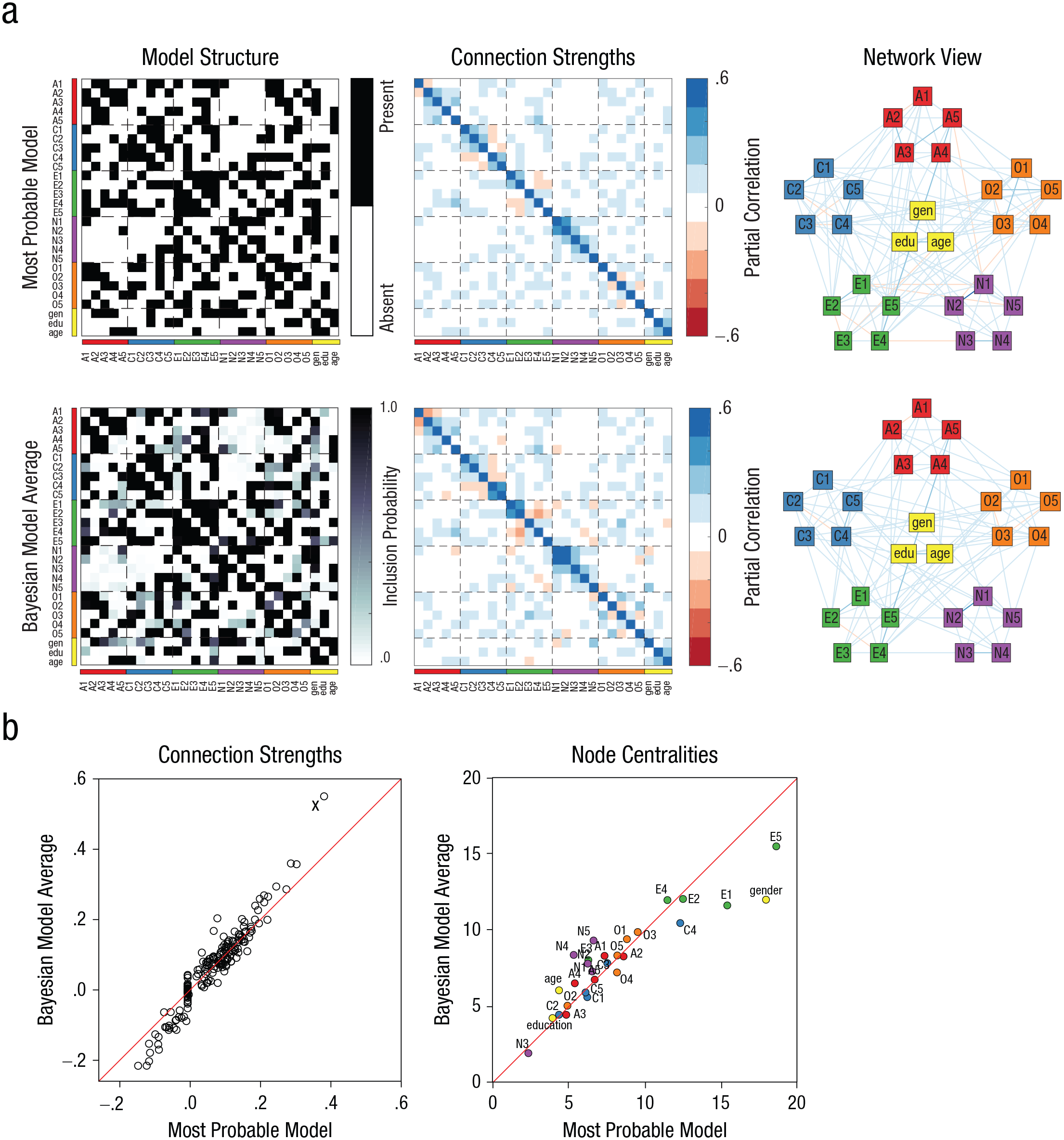
A comparison of network-analysis results obtained with model selection versus Bayesian model averaging (BMA) applied to the Big Five personality data set (Revelle, Wilt, & Rosenthal, 2010). The diagrams in (a) show a matrix indicating the variables connected (left), a matrix indicating the partial correlation for each connection (middle), and a network visualization of these partial correlations (right) for the maximum a posteriori estimated network (top row) and the BMA estimate (bottom row). The abbreviations for the variables in the models refer to specific items in the inventory, gender (“gen”), education (“edu”), and age. The scatterplots in (b) compare the strengths of all connections and betweenness centrality of all nodes for the BMA estimates and the most probable model. (The red lines indicate equality of the BMA estimates and the maximum a posteriori estimates.) A number of connections are estimated differently in the two approaches; the scatterplot on the left shows that the connection labeled “X” (the connection between item N1, “getting angry easily,” and item N2, “getting irritated easily”) has a partial correlation of .38 in the selected model and a partial correlation of .55 in the BMA estimate, and the scatterplot on the right shows that the centrality of gender and items E1 (“don’t talk a lot”) and E5 (“take charge”) is estimated differently by the two approaches.

The connection weights that correspond to a particular network structure can be seen as the parameters of a network model. There will be one set of these parameters that corresponds to the most likely model, but a more nuanced and accurate picture is obtained if one estimates the partial correlations while taking into account all other possible model structures as well—in other words, if one computes the Bayesian model average of the connection weights. These partial correlations can differ substantially from those in the most likely model (see Fig. 4b). For example, the connection between item N1 (“getting angry easily”) and item N2 (“getting irritated easily”) has a weight of .38 in the most likely model, but is estimated as .55 when the average is taken across all models. In other cases, partial correlations obtained with BMA are lower than those in the most likely model, because in many models those connections are absent. For instance, the connection between item O4 (“spend time reflecting on things”) and item N3 (“have frequent mood swings”) has a partial correlation of .09 in the most likely model, but only .01 in the BMA model.

These simple examples demonstrate the danger of selecting the best model as opposed to averaging across models in network analysis. The errors that model selection can induce propagate into subsequent analyses. For instance, it is commonplace in network analysis to compute centrality measures of the nodes in the network (Freeman, 1978; Opsahl, Agneessens, & Skvoretz, 2010). These measures represent the relative importance of the variables and the information flow on the network (Borgatti, 2005). Centrality can also be used to identify specific symptoms that may be the target of clinical treatment (Fried, Epskamp, Nesse, Tuerlinckx, & Borsboom, 2016; but see Dablander & Hinne, 2019). Of course, computing these indices using only the most likely model results in a ranking of the nodes that ignores any uncertainty about the network structure. Instead, one can compute the centrality score of each node for each model and weigh each score by the PMP of the corresponding model. This is the Bayesian model average of a derived quantity (the centrality measure), which is a deterministic function of the estimated parameters. Figure 4b shows the comparison of centrality measures computed on the most likely model versus those computed using BMA. Once again, a number of variables have different estimates if the Bayesian model ensemble is used instead of a single model. For example, the importance of the variables gender, E1 (“don’t talk a lot”), and E5 (“take charge”) is overestimated by the model-selection approach.

Limitations of Bayesian Model Averaging

BMA is particularly useful when researchers are interested in a particular parameter but do not know exactly how this parameter relates to the observations. In other words, they are uncertain about the underlying model. Consider the example from our introduction again; you are interested in the estimated arrival time of your train, not so much in the particulars of each considered scenario. Just as researchers are used to being explicit about the uncertainty of their parameter estimates—for example, by making predictions according to the posterior distribution rather than a point estimate—they should also be clear that they are rarely totally confident about which model best accounts for their data. Uncertainty about the model must also be taken into account, and the Bayesian framework defines an obvious and elegant way to do so. The resulting summary is the Bayesian-model-average estimate.

Of course, BMA is not without limitations. Given infinite data, Bayesian inference will identify one single model to be the true model. When this occurs, BMA provides parameter estimates according to this model only. This is desirable if the true data-generating model is one of the considered models (Vehtari & Ojanen, 2012; Vehtari, Simpson, Yao, & Gelman, 2019). If this is not the case, however, BMA will not identify the correct model. This occurs, for example, when one averages the predictions of discrete models, such as network structures (see the last example); this average is not predicted by any model (as the individual models predict only binary structures). However, it still has a clear and useful interpretation: It provides the inclusion probabilities of individual connections, which are similar to the inclusion probabilities of predictors in the generalized linear model. Furthermore, one can argue that model selection and averaging are not necessarily about identifying the true model, but rather are about identifying the model in which one should have the strongest belief, given one’s assumptions. The latter belief is conditioned on the data as well as the collection of models considered. (For a more in-depth discussion of this issue, we refer interested readers to Gronau & Wagenmakers, 2019a, 2019b.)

Although the BMA estimate of a parameter gives a more nuanced answer to a research question than model selection does, it is not a panacea. For instance, the BMA estimate of a partial correlation in network analysis is only a point estimate, summarizing the entire distribution of this parameter. That distribution likely consists of a spike at zero (for those models in which the corresponding connection is absent, and the partial correlation consequently is zero), and a bell curve centered around a nonzero value. The BMA summary does not reflect this, and hence may be misleading. The solution to this is to avoid point estimates whenever possible and work with the model-wise mixture distribution of the parameter instead, but of course this is often impractical.

A practical limitation of BMA is that, being Bayesian, the approach requires the specification of prior distributions both on parameters of each model and on the distribution of models themselves. Identifying appropriate prior distributions is not always straightforward, and even uniform or vague priors may have substantial influence on the outcome. This is essentially a critique of the Bayesian framework in general, and we refer readers to, for example, Wagenmakers et al. (2018) for more discussion on this topic. When one is in doubt, robustness checks can verify that conclusions do not depend on arbitrary choices of priors (van Doorn et al., 2019). Note that multimodel inference is also advocated in the frequentist framework, as it can reduce the bias due to placing too much confidence in a single model and provides more robust results (see, e.g., Burnham & Anderson, 2002, 2004; Claeskens & Hjort, 2008).

Finally, BMA can be computationally challenging, as enumerating candidate models quickly becomes intractable. Fortunately, for particular models such as the ones we have discussed here, approximate solutions, such as Markov chain Monte Carlo or adaptive sampling, are available.

Concluding Comments

BMA is the natural Bayesian way of dealing with uncertainty about both models and their respective parameters. It follows directly from the application of Bayes rule and provides several fundamental advantages compared with selecting the single most probable model.

We have outlined these advantages and provided three practical application examples. Of course, BMA is not limited to these scenarios and can be applied whenever there is model uncertainty. Other examples of BMA applications include the estimation of effect size (Haldane, 1932), linear regression (Clyde, Ghosh, & Littman, 2011), assessment of the replicability of effects (Iverson, Wagenmakers, & Lee, 2010), prediction in time-series analysis (Vosseler & Weber, 2018), analysis of the causal structure in a brain network (Penny et al., 2010), structural equation modeling (Kaplan & Lee, 2016), factor analysis (Dunson, 2006), and correcting for publication bias using the precision-effect test and precision-effect estimate with standard errors (Carter & McCullough, 2018). In general, BMA reduces overconfidence, results in optimal predictions (under mild conditions), avoids threshold-based all-or-nothing decision making, and is relatively robust against model misspecification.

We hope that this short example-driven introduction inspires researchers to consider the use of BMA in their statistical analyses. BMA gives due attention to uncertainty when competing models are compared, and this ultimately results in better predictions.

Supplemental Material

HinneOpenPracticesDisclosure – Supplemental material for A Conceptual Introduction to Bayesian Model Averaging

Supplemental material, HinneOpenPracticesDisclosure for A Conceptual Introduction to Bayesian Model Averaging by Max Hinne, Quentin F. Gronau, Don van den Bergh and Eric-Jan Wagenmakers in Advances in Methods and Practices in Psychological Science

Footnotes

Appendix: Bayesian Background

Bayesian statistics is increasingly gaining traction in psychological science (Andrews & Baguley, 2013; Hoijtink & Chow, 2017; Vandekerckhove et al., 2018), but as it is not yet mainstream, we provide a reference of key concepts and their mathematical definitions. Although these formal descriptions may safely be skipped for our main arguments, they provide the foundations of Bayesian statistics and are useful for understanding the statistical nuances of Bayesian model averaging.

Initial beliefs about a parameter of interest, say, the train delay t in the scenario with which we opened this article, are denoted by the prior distribution, p(t). Bayes rule is used to update these beliefs in light of data:

(1)

p ( t | data ) = p ( data | t ) p ( t ) p ( data ) .

Equation 1 provides the posterior distribution of t. In this equation, the role of the model, H, is often left implicit. To entertain multiple models however, one should explicitly condition the prior distribution on these and write instead

(2)

p ( t | data , H ) = p ( data | t , H ) p ( t | H ) p ( data | H ) .

Equation 2 formalizes that both prior beliefs about t and how t leads to observations depend on H. The marginal likelihood p(data|H) is the probability of the data under a given model. This can also be viewed as the probability of the data given the model, integrated across all possible parameter values, as follows:

(3)

p ( data | H ) = ∫ p ( data | t , H ) p ( t | H ) d t .

The Bayesian model average provides the posterior distribution (or the predictive distribution if one is predicting rather than estimating parameters) over t, regardless of any specific model. For instance, one might predict the current train delay on the basis of a number of scenarios and one’s observations. This is implemented by integrating out H:

(4)

p ( t | data ) = ∑ i p ( t | data , H i ) p ( H i | data ) .

In Equation 4, the estimates (predictions) of each model, p(t|data, H_i), are weighted by the posterior model probability, p(H_i|data), of the model. This term is obtained by once again applying Bayes rule, but at the level of models instead of parameters:

(5)

p ( H | data ) = p ( data | H ) p ( H ) ∑ i p ( data | H i ) p ( H i ) .

Note that what is called the model likelihood in the model posterior (Equation 5) is referred to as the marginal likelihood in the parameter posterior (Equation 2).

With these preliminaries, one arrives at an intuitive way of comparing two different models: One simply computes the ratio of the posterior model probability of the alternative model, H₁, relative to the posterior model probability of the null model, H₀. This gives

(6)

p ( H 1 | data ) p ( H 0 | data ) ︸ posterior model odds = p ( data | H 1 ) p ( data | H 0 ) ︸ Bayes factor × p ( H 1 ) p ( H 0 ) . ︸ prior model odds

The first term on the right-hand side of Equation 6 is the Bayes factor, often written as BF₁₀. It represents the update in beliefs about the comparison between H₁ and H₀ as a result of observations. Because it is often assumed that models are equally likely a priori—that is, p(H₁) = p(H₀)—the prior odds are 1 and the posterior odds are fully determined by the Bayes factor. The Bayes factor has an intuitive interpretation: It indicates how much more plausible the data are under H₁ compared with under H₀. Several authors have provided heuristics for the interpretation of the magnitude of Bayes factors (Jeffreys, 1939; Kass & Raftery, 1995).

If a large number of models are compared, listing all the pairwise Bayes factors becomes unwieldy. Furthermore, some of these models may be very similar to each other; for example, they may differ only in one of many predictors included in a linear model. In these situations, it is useful to compute a term’s posterior inclusion probability, which is simply the sum of the probabilities of the models that contain this term. To describe this probability thoroughly, let γ_i = 1 indicate that predictor x_i is included in a model, and let γ_i = 0 indicate the opposite case. Furthermore, let H ^ be the set of all models, so that with H ∈ H ^ : γ_i = 1, one selects the set of all models that contain predictor x_i. The posterior inclusion probability is then defined as

(7)

p ( γ i = 1 | data ) = ∑ H ∈ H ^ : γ i = 1 p ( H | data ) .

This probability is the sum of probabilities of all models that contain γ_i, which means it can also be interpreted as a Bayesian-model-average estimate of the presence of, as in this example, a predictor x_i. If one wants to draw conclusions about whether a predictor should be included, one computes the inclusion Bayes factor:

(8)

B F inclusion = ∑ H ∈ H ^ : γ i = 1 p ( data H ) ∑ H ∈ H ^ : γ i = 0 p ( data H ) ,

which indicates how much more likely the data are when the predictor is included, compared with when it is not included, regardless of specific model selections.

For more details on the application of Bayesian statistics in psychological science, we refer readers to, for example, Etz and Vandekerckhove (2018) and Wagenmakers et al. (2018).

Transparency

Action Editor: Frederick L. Oswald

Editor: Daniel J. Simons

ORCID iDs

Max Hinne

Eric-Jan Wagenmakers

Notes

References

Andrews

Baguley

(2013). Prior approval: The growth of Bayesian methods in psychology. British Journal of Mathematical and Statistical Psychology, 66, 1–7.

Appelbaum

Cooper

Kline

Mayo-Wilson

Nezu

Rao

(2018). Journal article reporting standards for quantitative research in psychology: The APA Publications and Communications Board task force report. American Psychologist, 73, 3–25.

Borgatti

S. P.

(2005). Centrality and network flow. Social Networks, 27, 55–71.

Burnham

K. P.

Anderson

D. R.

(2002). Model selection and multimodel inference: A practical information-theoretic approach (2nd ed.). New York, NY: Springer-Verlag.

Burnham

K. P.

Anderson

D. R.

(2004). Multimodel inference: Understanding AIC and BIC in model selection. Sociological Methods & Research, 33, 261–304.

Carter

E. C.

McCullough

M. E.

(2018). A simple, principled approach to combining evidence from meta-analysis and high-quality replications. Advances in Methods and Practices in Psychological Science, 1, 174–185.

Claeskens

Hjort

N. L.

(2008). Model selection and model averaging. Cambridge, England: Cambridge University Press.

Clyde

M. A.

Ghosh

Littman

M. L.

(2011). Bayesian adaptive sampling for variable selection and model averaging. Journal of Computational and Graphical Statistics, 20, 80–101.

Consonni

Fouskakis

Liseo

Ntzoufras

(2018). Prior distributions for objective Bayesian analysis. Bayesian Analysis, 13, 627–679.

10.

Cooper

Hedges

Valentine

(2009). The handbook of research synthesis and meta-analysis. New York, NY: Russell Sage Foundation.

11.

Dablander

Hinne

(2019). Node centrality measures are a poor substitute for causal inference. Scientific Reports, 9, Article 6846. doi:10.1038/s41598-019-43033-9

12.

Draper

(1995). Assessment and propagation of model uncertainty. Journal of the Royal Statistical Society: Series B (Methodological), 57, 45–97.

13.

Dunson

D. B.

(2006). Efficient Bayesian model averaging in factor analysis. Retrieved from ftp://webster.stat.duke.edu/pub/WorkingPapers/06-03.pdf

14.

Epskamp

Rhemtulla

Borsboom

(2017). Generalized network psychometrics: Combining network and latent variable models. Psychometrika, 82, 904–927.

15.

Etz

Vandekerckhove

(2018). Introduction to Bayesian inference for psychology. Psychonomic Bulletin & Review, 25, 5–34.

16.

Fragoso

T. M.

Bertoli

Louzada

(2018). Bayesian model averaging: A systematic review and conceptual classification. International Statistical Review, 86, 1–28.

17.

Freeman

L. C.

(1978). Centrality in social networks conceptual clarification. Social Networks, 1, 215–239.

18.

Fried

E. I.

Epskamp

Nesse

R. M.

Tuerlinckx

Borsboom

(2016). What are ‘good’ depression symptoms? Comparing the centrality of DSM and non-DSM symptoms of depression in a network analysis. Journal of Affective Disorders, 189, 314–320.

19.

Goldberg

L. R.

(1999). A broad-bandwidth, public-domain, personality inventory measuring the lower-level facets of several Five-Factor models. In Mervielde

Deary

I. J.

De Fruyt

Ostenfdorf

(Eds.), Personality psychology in Europe (Vol. 7, pp. 7–28). Tilburg, The Netherlands: Tilburg University Press.

20.

Gronau

Q. F.

Wagenmakers

E.-J.

(2020). Informed Bayesian t-tests. The American Statistician, 74, 137–143. doi:10.1080/00031305.2018.1562983

21.

Gronau

Q. F.

van Erp

Heck

D. W.

Cesario

Jonas

K. J.

Wagenmakers

E.-J.

(2017). A Bayesian model-averaged meta-analysis of the power pose effect with informed and default priors: The case of felt power. Comprehensive Results in Social Psychology, 2, 123–138.

22.

Gronau

Q. F.

Wagenmakers

E.-J.

(2019a). Limitations of Bayesian leave-one-out cross-validation for model selection. Computational Brain & Behavior, 2, 1–11.

23.

Gronau

Q. F.

Wagenmakers

E.-J.

(2019b). Rejoinder: More limitations of Bayesian leave-one-out cross-validation. Computational Brain & Behavior, 2, 35–47.

24.

Haldane

J. B.

(1932). The causes of evolution. Oxford, England: Macmillan.

25.

Heck

D. W.

Gronau

Q. F.

Wagenmakers

E.-J.

(2019). metaBMA: Bayesian model averaging for random and fixed effects meta-analysis (Version 0.6.2) [Computer software]. Retrieved from https://CRAN.R-project.org/package=metaBMA

26.

Hinne

Janssen

R. J.

Heskes

van Gerven

M. A. J.

(2015). Bayesian estimation of conditional independence graphs improves functional connectivity estimates. PLOS Computational Biology, 11(11), Article e1004534. doi:10.1371/journal.pcbi.1004534

27.

Hoeting

J. A.

Madigan

Raftery

A. E.

Volinsky

C. T.

(1999). Bayesian model averaging: A tutorial. Statistical Science, 14, 382–401.

28.

Hoijtink

Chow

S.-M.

(2017). Bayesian hypothesis testing: Editorial to the Special Issue on Bayesian data analysis. Psychological Methods, 22, 211–216.

29.

Iverson

G. J.

Wagenmakers

E.-J.

Lee

M. D.

(2010). A model-averaging approach to replication: The case of prep. Psychological Methods, 15, 172–181.

30.

Jeffreys

(1939). Theory of probability (1st ed.). Oxford, England: Oxford University Press.

31.

Jevons

W. S.

(1874). The principles of science: A treatise on logic and scientific method. London, England: Macmillan.

32.

Kaplan

Lee

(2016). Bayesian model averaging over directed acyclic graphs with implications for the predictive performance of structural equation models. Structural Equation Modeling: A Multidisciplinary Journal, 23, 343–353.

33.

Kaplan

Lee

(2018). Optimizing prediction using Bayesian model averaging: Examples using large-scale educational assessments. Evaluation Review, 42, 423–457.

34.

Kass

R. E.

Raftery

A. E.

(1995). Bayes factors. Journal of the American Statistical Association, 90, 773–795.

35.

Madigan

Raftery

A. E.

York

J. C.

Bradshaw

J. M.

Almond

R. G.

(1994). Strategies for graphical model selection. In Cheeseman

Oldford

R. W.

(Eds.), Selecting models from data (pp. 91–100). New York, NY: Springer.

36.

Marsman

Borsboom

Kruis

Epskamp

van Bork

Waldorp

L. J.

. . . Maris

(2018). An introduction to network psychometrics: Relating Ising network models to item response theory models. Multivariate Behavioral Research, 53, 15–35.

37.

Moghaddam

Khan

Murphy

K. P.

Marlin

B. M.

(2009). Accelerating Bayesian structural inference for non-decomposable Gaussian graphical models. In Bengio

Schuurmans

Lafferty

J. D.

Williams

C. K. I.

Culotta

(Eds.), Advances in Neural Information Processing Systems 22 (pp. 1285–1293). Vancouver, British Columbia, Canada: Curran Associates.

38.

Mohammadi

Dobra

(2017). The R package BDgraph for Bayesian structure learning in graphical models. ISBA Bulletin, 24(4), 11–16.

39.

Morey

R. D.

Rouder

J. N.

(2015). BayesFactor: Computation of Bayes factors for common designs (R package Version 0.9.12-4.2) [Computer software]. Retrieved from http://CRAN.R-project.org/package=BayesFactor

40.

Opsahl

Agneessens

Skvoretz

(2010). Node centrality in weighted networks: Generalizing degree and shortest paths. Social Networks, 32, 245–251.

41.

Penny

W. D.

Stephan

K. E.

Daunizeau

Rosa

M. J.

Friston

K. J.

Schofield

T. M.

Leff

A. P.

(2010). Comparing families of dynamic causal models. PLOS Computational Biology, 6(3), Article e1000709. doi:10.1371/journal.pcbi.1000709

42.

Petersen

S. E.

Sporns

(2015). Brain networks and cognitive architectures. Neuron, 88, 207–219.

43.

Revelle

Wilt

Rosenthal

(2010). Individual differences in cognition: New methods for examining the personality-cognition link. In Gruszka

Matthews

Szymura

(Eds.) Handbook of individual differences in cognition: attention, memory and executive control (pp. 27–49). New York, NY: Springer.

44.

Rouder

J. N.

Engelhardt

C. R.

McCabe

Morey

R. D.

(2016). Model comparison in ANOVA. Psychonomic Bulletin & Review, 23, 1779–1786.

45.

Rouder

J. N.

Morey

R. D.

Speckman

P. L.

Province

J. M.

(2012). Default Bayes factors for ANOVA designs. Journal of Mathematical Psychology, 56, 356–374.

46.

Rouder

J. N.

Morey

R. D.

Verhagen

Swagman

A. R.

Wagenmakers

E.-J.

(2017). Bayesian analysis of factorial designs. Psychological Methods, 22, 304–321.

47.

Roverato

(2002). Hyper inverse Wishart distribution for non-decomposable graphs and its application to Bayesian inference for Gaussian graphical models. Scandinavian Journal of Statistics, 29, 391–411.

48.

Scheibehenne

Gronau

Q. F.

Jamil

Wagenmakers

E.-J.

(2017). Fixed or random? A resolution through model averaging: Reply to Carlsson, Schimmack, Williams, and Bürkner (2017). Psychological Science, 28, 1698–1701.

49.

Schmidt

F. L.

(1992). What do data really mean? Research findings, meta-analysis and cumulative knowledge in psychology. American Psychologist, 47, 1173–1181.

50.

Selfridge

O. G.

(1959). Pandemonium: A paradigm for learning. In Blake

D. V.

Uttley

A. M.

(Eds.), Mechanisation of thought processes: Proceedings of a symposium held at the National Physical Laboratory on 24th, 25th, 26th and 27th November 1958 (Vol. 1, pp. 511–529). London, England: Her Majesty’s Stationery Office.

51.

Shen

Yang

Zhang

(2018). Benefits of expressive writing in reducing test anxiety: A randomized controlled trial in Chinese samples. PLOS ONE, 13(2), Article e0191779. doi:10.1371/journal.pone.0191779

52.

Smith

S. M.

Miller

K. L.

Salimi-Khorshidi

Webster

Beckmann

C. F.

Nichols

T. E.

. . . Woolrich

M. W.

(2011). Network modelling methods for fMRI. NeuroImage, 54, 875–891.

53.

Steel

M. F. J.

(in press). Model averaging and its use in economics. Journal of Economic Literature.

54.

Strack

Martin

L. L.

Stepper

(1988). Inhibiting and facilitating conditions of the human smile: A nonobtrusive test of the facial feedback hypothesis. Journal of Personality and Social Psychology, 54, 768–777.

55.

Vandekerckhove

Rouder

J. N.

Kruschke

J. K.

(2018). Editorial: Bayesian methods for advancing psychological science. Psychonomic Bulletin & Review, 25, 1–4.

56.

van der Maas

H. L. J.

Kan

K.-J.

Marsman

Stevenson

C. E.

(2017). Network models for cognitive development and intelligence. Journal of Intelligence, 5(2), 1–17.

57.

van Doorn

van den Bergh

Boh

Dablander

Derks

Draws

. . . Wagenmakers

E.-J.

(2019). The JASP guidelines for conducting and reporting a Bayesian analysis. PsyArXiv. doi:10.31234/osf.io/yqxfr

58.

Vehtari

Ojanen

(2012). A survey of Bayesian predictive methods for model assessment, selection and comparison. Statistics Surveys, 6, 142–228.

59.

Vehtari

Simpson

D. P.

Yao

Gelman

(2019). Limitations of “limitations of Bayesian leave-one-out cross-validation for model selection.” Computational Brain & Behavior, 2, 22–27.

60.

Vosseler

Weber

(2018). Forecasting seasonal time series data: A Bayesian model averaging approach. Computational Statistics, 33, 1733–1765.

61.

Wagenmakers

E.-J.

Beek

Dijkhoff

Gronau

Q. F.

Acosta

Adams

R. B.

Jr. . . . Zwaan

R. A.

(2016). Registered Replication Report: Strack, Martin, & Stepper (1988). Perspectives on Psychological Science, 11, 917–928.

62.

Wagenmakers

E.-J.

Marsman

Jamil

Verhagen

Love

. . . Morey

R. D.

(2018). Bayesian inference for psychology: Part I: Theoretical advantages and practical ramifications. Psychonomic Bulletin & Review, 25, 35–57.

63.

Wilson

M. A.

Iversen

E. S.

Clyde

M. A.

Schmidler

S. C.

Schildkraut

J. M.

(2010). Bayesian model search and multilevel inference for SNP association studies. The Annals of Applied Statistics, 4, 1342–1364.

64.

Zellner

Siow

(1980). Posterior odds ratios for selected regression hypotheses. In Bernardo

J. M.

DeGroot

M. H.

Lindley

D. V.

Smith

A. F. M.

(Eds.), Bayesian statistics: Proceedings of the First International Meeting held in Valencia (Spain) (pp. 585–603). Valencia, Spain: University Press.

Supplementary Material

Please find the following supplemental material available below.

For Open Access articles published under a Creative Commons License, all supplemental material carries the same license as the article it is associated with.

For non-Open Access articles published, all supplemental material carries a non-exclusive license, and permission requests for re-use of supplemental material or any part of supplemental material shall be sent directly to the copyright owner as specified in the copyright notice associated with the article.

0.00 MB

0.64 MB