Sage Journals: Discover world-class research

Abstract

Drift-diffusion models (DDMs) are pivotal in understanding evidence-accumulation processes during decision-making across psychology, behavioral economics, neuroscience, and psychiatry. Hierarchical DDMs (HDDMs), a Python library for hierarchical Bayesian estimation of DDMs, has been widely used among researchers, including researchers with limited coding proficiency, in fitting DDMs and other sequential sampling models. However, issues of compatibility in installation and lack of support for more recent Bayesian-modeling functionalities pose serious challenges for new users, limiting broader adaptation and reproducibility of HDDMs. To address these issues, we created dockerHDDM, a user-friendly computational environment for HDDMs with new features. dockerHDDM brings three improvements: (a) easy to install once docker is installed, ensuring reproducibility and saving time for researchers; (b) compatible with machines with Apple chips; (c) seamless integration with ArviZ, a state-of-the-art Bayesian-modeling library. This tutorial serves as a practical, hands-on guide for researchers to leverage dockerHDDM’s capabilities in conducting efficient Bayesian hierarchical analysis of DDMs. The notebook presented here and in the docker image will enable researchers with various programming levels to model their data with HDDMs.

Keywords

HDDM drift-diffusion models Bayesian hierarchical modeling reproducibility docker Python open data open materials

The drift-diffusion model (DDM) is one of the most widely used computational models (for an overview, see Ratcliff et al., 2016) to quantify the evidence-accumulation processes during decision-making in neuroscience (Cavanagh et al., 2011; Herz et al., 2017; Shadlen & Shohamy, 2016), psychology (Hu et al., 2020; D. J. Johnson et al., 2017; Kutlikova et al., 2023), behavioral economics (Desai & Krajbich, 2022; Sheng et al., 2020), and psychiatry (Ging-Jehli et al., 2021; Pedersen et al., 2022). According to the DDM, experimentally observed pairs of response times and choices arise from a process of stochastic evidence accumulation to a decision boundary (e.g., Voss et al., 2013; see Figure 1 and the related DDM glossary in Table 1). This theoretical framework has been shown not only to correlate robustly with established neural substrates (Chandrasekaran et al., 2017; Forstmann et al., 2016) but also to serve as a powerful measurement tool for examining individual differences across cognitive tasks, experimental manipulations, and participant populations (Boag et al., 2024; Donkin & Brown, 2018; Evans & Wagenmakers, 2020; but see Liu et al., 2023). Despite its theoretical contributions, the DDM is difficult to apply to experimental data in practice because the derivation of inference-relevant quantities (e.g., the likelihood function) requires a mathematical understanding of the complex stochastic process of evidence accumulation.

Fig. 1.

Illustration of the evidence-accumulation process assumed by the drift-diffusion model (DDM). DDM has four basic parameters: drift rate ( $v$ ), decision boundary ( $a$ ), initial bias ( $z$ ), and nondecision time ( $t$ ). The drift rate ( $v$ ) is the average speed of evidence accumulation toward a decision; the decision boundary ( $a$ ) is the distance between two decision thresholds, and the evidence needed to make a decision increase as $a$ increases; the initial bias ( $z$ ) reflects the starting point of evidence accumulation; nondecision time ( $t$ ) is the time not used for evidence accumulation, for example, stimulus encoding or motor execution. For a more detailed description of the DDM and its parameters, see Table 1.

Table 1.

Drift-Diffusion Model Glossary

Term	Description
Accumulator	A component of the DDM that accumulates evidence for different decision options until a threshold is reached, triggering a decision.
Random walk	A stochastic process that describes a path consisting of a sequence of random steps. It refers to the modeling of decision-making as a process of accumulating evidence over time.
Diffusion	The diffusion refers to the variability in the evidence-accumulation process that represents random fluctuations in the decision variable.
Optional stopping	The concept of stopping the decision-making process at a point chosen by the decision maker, often when a certain level of confidence or evidence threshold is reached.
Drift rate ( $v$ )	The average rate of evidence accumulation toward one of the decision boundaries. The more difficult the task, the less stimulus discrimination and the smaller the drift rate.
Decision boundary ( $a$ )	The threshold that, when reached by the accumulated evidence, triggers a decision. It represents the speed-accuracy trade-off or caution, and the higher its value, the higher the accuracy at the expense of slower response times.
Nondecision time ( $t$ )	The time taken by processes other than decision-making (e.g., sensory encoding and motor execution). It simply shifts response time distribution.
Initial bias ( $z$ )	The initial value of the decision variable, which indicates any initial bias in evidence accumulation, is also called ‘starting point’ in the literature. The closer it is to a boundary (1 and 0 correspond to the upper and lower boundaries, respectively), the faster and more frequent the response.
Drift-rate variability ( $s v$ )	The variability in the drift-rate parameter across trials. It increases the proportion of slow errors.
Initial bias variability ( $s z$ )	The across-trial variability in the initial bias parameter in the DDM. It increases the proportion of fast errors.
Nondecision-time variability ( $s t$ )	The across-trial variability in the nondecision time parameter in the DDM. It simultaneously increases the probability of both faster and slower responses, resulting in a thicker tail of the RT distribution.

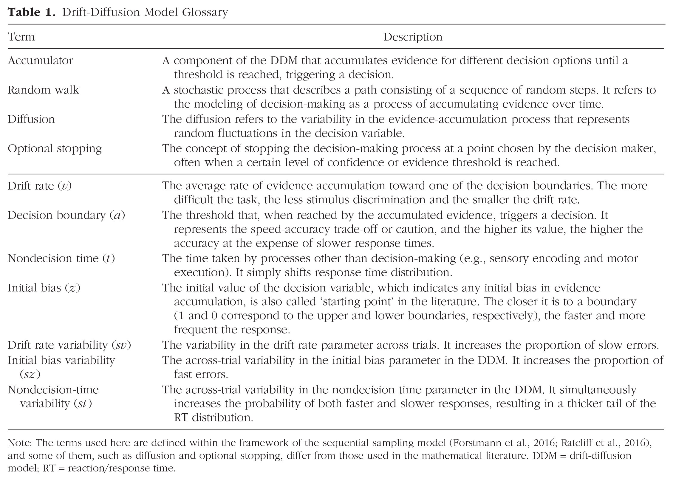
Note: The terms used here are defined within the framework of the sequential sampling model (Forstmann et al., 2016; Ratcliff et al., 2016), and some of them, such as diffusion and optional stopping, differ from those used in the mathematical literature. DDM = drift-diffusion model; RT = reaction/response time.

Several software packages have been developed to facilitate the application of DDM (see “Why Use dockerHDDM Among Tools” section), proving particularly beneficial for researchers with limited computational expertise. Among them, HDDM, a Python library for hierarchical DDM, is by far the most cited toolbox in the community (Wiecki et al., 2013; with 996 citations in Google Scholar as of August 26, 2024). Despite the success and popularity of HDDM, it suffers from several practical issues. First, the installation process of HDDM is cumbersome, exacerbated by its reliance on PyMC 2.3.8 for Markov chain Monte Carlo (MCMC) sampling, a package that is no longer supported and may clash with the latest computer modules. Second, and for the same reason, out-of-the-box HDDM is not compatible with Apple chips, which creates a significant barrier for Mac users. Third, although HDDM natively centers around Bayesian methods, it does not conveniently support all aspects of the evolved standards in Bayesian-modeling workflows (Ahn et al., 2017; Gelman et al., 2020; Kruschke, 2021). Significant progress has recently been made in supporting the principled Bayesian-modeling workflow in easy-to-use tool kits, such as the Python package ArviZ (Kumar et al., 2019). Bridging these new capabilities with HDDM facilitates a one-stop Bayesian-modeling pipeline for experimentalists and computational modelers interested in applying the DDM to their experimental data.

To address the above issues, we leveraged the Docker container technology to create dockerHDDM, a stable and complete virtualized Python computing environment that enables out-of-the-box implementations of Bayesian hierarchical DDMs. dockerHDDM has three major advantages (Table 2). First, it benefits from the easy-to-deploy nature of the Docker environment to avoid compatibility issues. Second, it is compatible with both Intel and Apple chips. Third, it augments HDDM with ArviZ, a Python module that enables a wide range of advanced Bayesian-modeling analyses. We expect dockerHDDM to provide an easy-to-use environment to help researchers across various backgrounds efficiently use DDM in their research.

Table 2.

Comparisons Between dockerHDDM and the Original HDDM Package

	HDDM	dockerHDDM
Support ArviZ^a	No	Yes
Plotting (e.g., HDI)	No	Yes
Diagnosis (e.g., ESS)	No	Yes
Model comparison (LOO-CV, WAIC)	No	Yes
Installation	Hard	Easy
Parallel processing	Hard	Easy
Compatibility with Apple chips	Hard	Easy

Note: HDI = high-density interval; ESS = effective sample size; LOO-CV = leave-one-out cross-validation; WAIC, widely applicable information criterion; PPC, posterior predictive checks.

Plotting, diagnosis, and model comparison are functions of ArviZ, including HDI, ESS, LOO, WAIC, and PPC.

How to Follow This Tutorial

The primary goal of this article is to present a practical guide to dockerHDDM for beginners with little modeling experience. In the tutorial, we start with step-by-step instructions on how to configure the dockerHDDM environment and how to use it in practical data analysis (Fig. 2). To assist reproducibility and easy application, a corresponding step-by-step video walk-through is available on YouTube at https://www.youtube.com/watch?v=ZU1fbXEuP8s or on OSF at https://osf.io/xz9m2.

Fig. 2.

dockerHDDM usage flowchart. The code in the figure is for demonstration purposes only. Specific instructions and copyable code can be found in the following corresponding sections. The top panel describes how to install Docker, corresponding to “Install Docker”; the middle panel describes how to pull and run dockerHDDM, corresponding to “Pull dockerHDDM Image” and “Run dockerHDDM Container”; and the bottom panel shows the workflow in dockerHDDM, corresponding to “Example of Workflow.” A video tutorial is available at https://www.youtube.com/watch?v=ZU1fbXEuP8s and https://osf.io/xz9m2.

Box 1.

Glossary of Terms Used in Bayesian Modeling

Prior, or prior distribution, often referred to as $p (θ)$ , is the initial belief that researchers have from pilot data.

Likelihood, or likelihood function, often referred to as $p (y | θ)$ , is the probability of the observed data $y$ as a function of the specific parameters $θ$ of a chosen statistical model. For example, the Bernoulli function is the likelihood function for statistically describing coin tossing.

Posterior, or posterior distribution, often referred to as $p (θ | y)$ , refers to the updated beliefs about the parameters $θ$ after observing the data $y$ , balancing prior knowledge with observed data according to Bayes’s rule, that is, $p (θ | y) \propto p (y | θ) p (θ)$ .

Markov chain Monte Carlo (MCMC) is a sampling method to infer the posterior distribution by simulation. The Markov chains (usually multiple MCMC chains are required) are algorithmically constructed so that their corresponding stationary distribution using MCMC samples matches the posterior distribution of interest in the limit (Kruschke, 2014; Robert & Casella, 2004). The process of reaching this stationary distribution is called “MCMC convergence.” These sampled parameter values serve as the approximation to the posterior distribution and can then be used to obtain empirical estimates of the posterior distribution and associated summary statistics of interest using Monte Carlo integration. In the literature, a chain (or trace) is referred to as a collection of samples (or draws). Traces serve as a basis for diagnosing convergence and/or other potential problems with the procedure in a given application. MCMC is particularly useful for models with high complexity.

Effective sample size (ESS) is the number of independent samples with the same estimation power as the N autocorrelated samples from each MCMC chain. ESS is often used to determine whether the number of draws in MCMC chains is sufficient to guarantee a reliable estimate of uncertainty. An ESS greater than 400 is recommended, with the ESS for all four MCMC chains being 100 (Vehtari et al., 2021). However, the required ESS should be informed by the statistics one wishes to estimate from the posterior. It is recommended that an ESS of at least 10,000 is required for reasonably stable estimates of highest density intervals; for stable estimates of equal-tailed intervals, a lower ESS is sufficient; a smaller ESS may yield stable estimates of the central tendency, especially if it falls in a high-density region of the distribution (Kruschke, 2018, 2021).

Gelman-Rubin statistics ( $\hat{R}$ ) is the ratio of within-chains variability to between-chains variability. Values close to 1.0 for all parameters and quantities of interest suggest that the MCMC algorithm has sufficiently converged to stationary distributions. In practice, the maximum $\hat{R}$ must be less than 1.1 (Annis et al., 2017), more stringent criteria requires the $\hat{R}$ values of less than 1.01, and a compromise is 1.05 (A. A. Johnson et al., 2022).

Posterior predictive samples, $p (\tilde{y} | y)$ , simulates new data $\tilde{y}$ conditional on the posterior distribution given the observed data $y$ . The simulated data can then be used to check whether the model can be considered a good fit to the data-generating mechanism by comparing the simulation with the observed data. This process is often called “posterior predictive checks.”

Leave-one-out cross-validation is a model-evaluation approach in which the model is trained on all observations except for a single observation $y_{i}$ (where $i = 1, 2, 3, \dots, n$ ), and then used to predict the held-out observation $y_{i}$ . This procedure is repeated for each of the n observations.

Log predictive density, $l o g p (\tilde{y} | θ)$ , is an overall summary of a model’s predictive abilities by estimating the log-likelihood of new data $\tilde{y}$ given the true parameters $θ$ . However, because both the new data $\tilde{y}$ and the true-model parameters $θ$ are typically unavailable in empirical data, the log predictive density is approximated using the observed data $y$ and the posterior estimates of the parameters $\hat{θ}$ , hence $l o g p (\tilde{y} | θ) \approx l o g p (y | \hat{θ})$ . This estimate, when multiplied by −2, gives the deviance, $- 2 l o g p (y | \hat{θ})$ . However, because $l o g p (y | \hat{θ})$ is a biased estimate of $l o g p (\tilde{y} | θ)$ , an adjustment is required to correct the bias.

Log pointwise predictive density, $\sum_{i = 1}^{n} l o g (\frac{1}{S} \sum_{s = 1}^{S} p (y_{i} | θ^{s}))$ , is the likelihood of each observed data point $y_{i}$ conditional on the model parameters $θ^{s}$ . In practice, this quantity is estimated using samples $θ^{s}$ (for $s = 1, 2, 3, \dots, S$ ) drawn from the posterior distribution.

Expected log pointwise predictive density (ELPPD), $\sum_{i = 1}^{n} E_{f} (l o g p_{p o s t} ({\tilde{y}}_{i}))$ , is a measure of out-of-sample predictive performance for new data ${\tilde{y}}_{i}$ generated by the true data-generating process. $p_{p o s t} ({\tilde{y}}_{i})$ is the predictive density for ${\tilde{y}}_{i}$ based on the posterior distribution, f is the true underlying model, and $E_{f}$ denotes the expectation that averages over the true data-generating distribution (Gelman et al., 2014). ELPPD is commonly the unknown parameters $θ$ in a model before observing data. It can either be formed from existing research or used to compare the predictive performance of different models because it provides an estimate of how well a model is expected to perform on new data.

Highest density interval (HDI) is an estimate of a parameter’s credible range in the context of Bayesian statistics. It encompasses an interval of the posterior distribution in which each point within this interval has a higher density than points outside of it. For instance, a 95% HDI means that there is a 95% chance that the true parameter value falls within this range, making it a reliable indicator of parameter uncertainty. HDIs are commonly used for hypothesis testing regarding effect sizes and comparisons across different conditions or groups.

A region of practical equivalence (ROPE) is a predefined range of parameter values that are considered practically equivalent to zero, which could be based on existing literature or theoretical reasoning (Kruschke, 2018, 2021). To determine whether a parameter estimate is significantly different from zero, a ROPE might be set as a range around zero. If the 95% HDI of the parameter lies entirely outside this ROPE, the parameter is considered credibly different from zero. If the HDI is entirely within the ROPE, the parameter is effectively zero for practical purposes. Partial overlap suggests that the parameter’s result should be interpreted with caution. Note that caution should be taken when using the HDI + ROPE method for statistical inference on transformed parameters because of an inconsistency in transformation properties between ROPE and HDI (Etz et al., 2024).

Bayes factor (BF) and Savage-Dickey density ratio (SDDR): BF quantifies the strength of evidence for one statistical model over another. A value greater than 1 suggests more support for the alternative model relative to the original model, offering a continuous measure of evidence (Kass & Raftery, 1995). The SDDR simplifies BF computation for nested models by comparing a parameter’s posterior density at a specific point (typically zero) to its prior density at the same point. This method is efficient and effective for evaluating whether a parameter is significantly different from zero (Wagenmakers et al., 2010).

In the setup section (top panel in Fig. 2, corresponding to “Install Docker” section in this article), we provide instructions on how to install Docker. After that, we demonstrate how to obtain the dockerHDDM image and how to use this image to access the Jupyter notebook interface (middle panel in Fig. 2, corresponding to “Pull dockerHDDM Image” and “Run dockerHDDM Container” sections). Finally, within a working Jupyter notebook, we show how to analyze an example data set with dockerHDDM in a principled Bayesian workflow (bottom panel in Fig. 2, corresponding to “Example of Workflow” section).

Install and use dockerHDDM

Install Docker

Docker serves to create an all-in-one, fast, cross-platform computing environment. The Docker website provides easy-to-follow installation instructions (https://docs.docker.com/get-docker/) and supports Windows, MacOS, and Linux (see Box 2). Windows users should ensure their system version is 21H2 (build 19044) or higher and have either WSL or Hyper-V configured before installation (see https://docs.docker.com/desktop/install/windows-install/).

Box 2.

Basic Introduction to Docker

Docker is an open-source platform that automates the deployment, scaling, and management of applications. It achieves this through containerization, a process that packages an application and its dependencies into a single, portable, and consistent unit, known as a “container image.” Containers ensure that applications run reliably regardless of the environment (Peikert & Brandmaier, 2021; Wiebels & Moreau, 2021).

Docker uses a client-server architecture in which the Docker client communicates with the Docker daemon, responsible for building, running, and distributing containers. The core components of Docker are the Docker Engine, Docker Hub, and Docker Compose. The Docker Engine is the runtime that enables containerization, and Docker Hub is a cloud-based registry for sharing and managing container images. Docker Compose, on the other hand, is a tool for defining and running multicontainer Docker applications.

Common Docker Commands:

➢ `docker pull [image]`: Downloads a Docker image from a registry. For instructions on downloading the dockerHDDM image, see “Pull dockerHDDM Image.”

➢ `docker run [image]`: Runs a container from a Docker image. For details on how to start a container using the dockerHDDM image, see “Run dockerHDDM Container.”

➢ `docker images`: Lists all Docker images on the local machine. This can be used to check different versions of the dockerHDDM image.

➢ `docker commit [container_id] [new_image_name]`: Creates a new image from a container’s changes. For example, if you modify or install new Python packages in the dockerHDDM container, you can save these changes as a new image.

➢ `docker build [dockerfile]`: Builds a Docker image from a Dockerfile in the current directory. You can customize the dockerHDDM image using the provided Dockerfile.

➢ `docker push [repository/image:tag]`: Uploads a Docker image to a registry. After logging in, you can push the saved image to Docker Hub or any other Docker registry.

➢ `docker rmi [image]`: Removes a Docker image from the local machine. This is useful for cleaning up unused images.

➢ `docker save -o [output_file] [image]`: Saves a Docker image to a tar archive file. This is useful for backing up images or transferring them to another system.

➢ `docker load -i [input_file]`: Loads a Docker image from a tar archive file. This can be used to restore or import images from a backup.

After installing Docker Desktop (or Docker Engine for Linux users), one can verify the installation by running the following command in a terminal (Fig. 3). If the container starts and runs successfully, it will display a confirmation message and then exit (Fig. 3):

$ docker run hello-world

Fig. 3.

Command to check Docker installation in terminal. After running the command `docker run hello-world` (highlighted at first line), the printout shows that Docker has been successfully installed on the system. The schematic interfaces of the terminal on different platforms are shown: (left) MacOS, (middle) Windows, and (right) Ubuntu.

Pull dockerHDDM image

After ensuring that Docker has been successfully installed and the Docker engine is running (Fig. 3), you can pull the dockerHDDM image by simply running the command in the terminal (see the meaning of each argument in Fig. 4a):

$ docker pull hcp4715/hddm

$ docker pull hcp4715/hddm:latest

This command will pull the latest default version of dockerHDDM, which corresponds to the image with the tag `1.0.1`. One can also select different tags for different versions of HDDM (see https://hub.docker.com/r/hcp4715/hddm/tags). Note that the tutorial in this article works with the `latest` or `1.0.1` tags, and it is compatible with 0.8.0, with minor grammar changes.

Fig. 4.

Docker commands to download and run dockerHDDM. (a) Download/pull dockerHDDM from the Docker hub. The command by default downloads the latest version of `hcp4715/dockerHDDM` if the image tag is not specified. The CPU architecture (Apple or Intel chips, corresponding to ARM64 and AMD64 architectures, respectively) is automatically recognized when the image is downloaded. (b) Command to start a container. Note, “\” separates different lines of a command in Linux and MacOS terminals but not in Windows.

Run dockerHDDM container

After pulling the Docker image to a local machine, you can start a computing environment by running the dockerHDDM image with the command in the terminal (Fig. 4b):

This command creates a Docker container, which is a specialized environment encapsulated within the Docker platform. The `-v` option is used to mount a local folder into the container’s file system, enabling file exchange from the host machine. The example code `$(pwd):/home/jovyan/work` specifies two paths separated by a colon. The path on the left, denoted by `$(pwd)`, represents the current working directory on the host machine, and the path on the right, `/home/jovyan/work`,¹ is the location inside the container where the folder will be mounted (Fig. 4b). This means that you can read and write the files from your local machine in the “work” directory in the browser. `$(pwd)` can be replaced with a valid folder path on your local machine. For example, for a folder named “ddm_project” on the drive D, it can be mounted with the following arguments in the respective operating systems: in Linux, `-v /mnt/d/ddm_project:/home/jovyan/work`; in Windows, `-v D:\ddm_project:/home/jovyan/work`; and in MacOS, `-v /Volumes/D/ddm_project:/home/jovyan/work`. The other arguments in the command are explained in Fig. 4b.

After running the `docker run . . .` command, a URL appears at the end of the terminal output (Fig. 2, middle panel). You can copy and paste this URL “http://127.0.0.1:8888/?token=. . .” into any web browser (e.g., Firefox or Chrome) to launch a Jupyter interface based on the dockerHDDM container. If the URL does not load properly, check whether port 8888 is being used by other Docker containers or programs. If so, close those containers or programs. Alternatively, you may change the port, for example, use port 7777 (i.e., set `-p 7777:8888`); in this case, you should replace the “8888” in the URL to “7777” (e.g., “http://127.0.0.1:7777/?token=. . .”). You can then open or initialize a Jupyter notebook² to code, run, and view the output directly. Note that the `--rm` flag included in the command means that the dockerHDDM container, along with any data or newly installed Python modules, will be deleted when the container stops. However, any files or data mounted to the container from the `$(pwd)` path will remain unaffected. This ensures the reproducibility of the computing environment. If you wish to modify the computing environment, for example, by installing additional Python modules, we recommend that you first read the Docker API before removing `--rm` directly.

In the Jupyter interface, you will find two files and two folders (Fig. 2, middle). The notebook dockerHDDM_Workflow.ipynb offers a detailed reproduction of the analyses presented in this article, which we discuss further in “Example of Workflow.” In contrast, the notebook dockerHDDM_Quick_View.ipynb provides a brief overview of the dockerHDDM image’s new features and an introduction to basic modeling processes. One folder is “work,” which mounts the local path into the docker environment. The other folder, “OfficialTutorials,” contains notebooks that reproduce the official tutorials available at https://hddm.readthedocs.io/en/latest/tutorials.html. Beginners can follow HDDM_Basic_Tutorial.ipynb to get a basic understanding of HDDM, as discussed in Wiecki et al. (2013); HDDM_Regression_Stimcoding.ipynb covers more advanced models with regression, in which parameters can vary based on experimental conditions and other covariates; Posterior_Predictive_Checks.ipynb introduces posterior predictive checks (PPCs), showing how to generate predicted data from fitted parameter posteriors and how to analyze these predicted data; LAN_Tutorial.ipynb introduces advanced use of LAN functions that address the problematic likelihood of more complicated models based on neural-network methods (Fengler et al., 2021).

Novel Features of dockerHDDM

The dockerHDDM_Quick_View.ipynb illustrates two novel features in dockerHDDM (compared with HDDM installed directly without Docker): parallel computing for MCMC chains and creating InferenceData data for ArivZ analyses (as shown in the <Code Block 1>):

For all models defined by methods such as `hddm.HDDM()` or `hddm.HDDMRegressor()`, the user can employ the `.sample()` method to run the MCMC algorithm for model fitting. The original HDDM provided two main parameters to set the MCMC algorithm; the first parameter was the number of samples (`500`), and the second was the number of burn-ins (`burn=100`).³

In dockerHDDM, we included five extra arguments in `.sample()` method to provide parallel computing for MCMC chains and create InferenceData.

To preserve compatibility and consistent output with origin HDDM, the arguments are configured with the following defaults: `return_infdata=False`, `sample_prior=False`, `loglike=False`, `ppc=False`, `save_name=None`, and `chains=1`.

The `chains` argument determines the number of MCMC chains. Using more than two chains triggers multithreaded parallel computation, which can significantly reduce the time when multiple chains are needed to compute model diagnosis index $\hat{R}$ (see “Model Diagnosis”). The number of parallel MCMC chains is limited by the number of available CPU cores/threads available. For example, the maximum number of chains for a computer with four cores (eight threads) is eight. Setting the “chains” argument more than eight may degrade performance. Nonetheless, whenever possible, a number of four chains is commonly used.

The `return_infdata`argument converts HDDM results into the InferenceData structure,⁴ accessible via `model.infdata`, by default set to `False` to maintain compatibility with original HDDM output. In addition, we have included `loglike` for computing and saving log-likelihood values (see “Model Comparison”), `ppc` for PPCs (see “PPC”), and `sample_prior=True` for calculating Savage-Dickey density ratio (Wagenmakers et al., 2010) to approximate Bayes factor (BF; see “Statistical Inference”). When setting `ppc` as `True`, it defaults to generating 500 predictions for each observed data, but users can adjust this by adding argument `n_ppc`. Likewise, when setting `sample_prior` as `True`, it defaults to sampling 2,000 draws for each prior parameter, but users can adjust this by adding argument `n_prior`.

Finally, the `save_name` argument specifies the path and file name for saving the model and InferenceData, which is convenient for reusing results. One can load the model using `model = hddm.load(‘example.hddm’)` and the InferenceData with `infdata = az.from_netcdf(‘example.nc’)`.

Example of Workflow

In this section (Fig. 2, bottom panel), we demonstrate how to use dockerHDDM (i.e., HDDM and ArviZ) to perform key steps of Bayesian modeling (Gelman et al., 2020; Martin et al., 2024): model specification and fitting, model diagnosis, model comparison, PPC, and statistical inference. The code reproduced in this section can be found in dockerHDDM_Workflow.ipynb in the dockerHDDM environment.

Example Data

For convenience, we use the data from Cavanagh et al. (2011), which is built within HDDM, as an example to demonstrate how to implement the modeling workflow. This data set contains response time and choice data from 14 Parkinson’s patients (see Table 3). In the experiment, participants were asked to choose between two options associated with either high or low reward values (i.e., reward probabilities in typical reinforcement-learning tasks). The relative value differences between the two options define two levels of conflict: high conflict for low-low and high-high trials (“HC” in variable “conf”) and low conflict for low-high trials (“LC” in variable “conf”).

Table 3.

Example Data Set From Cavanagh et al. (2011)

rt	response	conf
1.21	1.0	HC
1.63	1.0	LC
1.03	1.0	HC
2.77	1.0	LC
1.14	0.0	HC

Note: The data structure required for HDDM is long-format data, where each row represents one trial. “subj_idx” is the subject index, “rt” is the response time (in seconds), and “response” in this case represents the accuracy, where 1 is correct and 0 is incorrect. These three columns of data are mandatory when using HDDM and must be kept consistent with the column names and the units (rt, seconds). “conf” is an optional variable, corresponding to the conflict level, where “HC” denotes high conflict and “LC” denotes low conflict. “conf” is not a mandatory variable or column, meaning that different factor names and levels can be used depending on the experimental design. In addition, multiple variables may be maintained in the data, which may be categorical or continuous.

Note that HDDM requires the inclusion of three columns of variables, “subj_idx,” “rt,” and “response,” to construct the hierarchical model. This means that when analyzing your own data, these three columns of variables must appear in the data set with identical column names. In addition, the unit of “rt” must be seconds, and “response” is coded as 1 for the upper boundary of the corresponding choice and 0 for the lower boundary (for more details, see https://hddm.readthedocs.io/en/latest/howto.html).

Model Specification

As a demonstration of model specification, we test an example question: Is there an effect of conflict levels on drift rate (Wiecki et al., 2013). To answer the question, we constructed three computational models (see Table 4).

Table 4.

Models Used in This Tutorial

Models	Describe	HDDM functions for defining a model (`df` is the data from Cavanagh et al., 2011)	n params
Model 0	Baseline	hddm.HDDM(df, include=[‘a’, ‘v’, ‘t’, ‘z’, ‘sv’, ‘sz’, ‘st’])	67
Model 1	Varying drift rates across conditions	hddm.HDDM(df, include=[‘a’, ‘v’, ‘t’, ’z’, ‘sv’, ‘st’, ‘sz’], depends_on={‘v’: ‘conf’})	82
Model 2	Varying within-subjects drift rates across conditions	hddm.HDDMRegressor(df, “v ~ 1 + C(conf, Treatment(‘LC’))”, group_only_regressors=False, keep_regressor_trace=True, include=[‘a’, ‘v’, ‘t’, ‘z’, ‘sv’, ‘st’, ‘sz’])	83

Note: `hddm.HDDM()` is the default function for constructing a hierarchical drift-diffusion model. The `include` argument allows the addition of free parameters, which are fixed by default. The `depends_on` argument specifies a parameter (e.g., v) that depends on a categorical independent variable (e.g., ‘conf’). The `hddm.HDDMRegressor()` is an HDDM function that includes effects of conditions in a linear regression fashion. The `keep_regressor_trace` argument allows a trace of the regressor to be kept, which is needed for posterior predictive checks. By default, the hierarchical regression allows only the intercept to vary across participants, and the slope is fixed at the population level. The `group_only_regressors = FALSE` argument additionally estimates the slopes at the individual level in the regression model.

Model 0 served as the baseline without considering the effect of conflict level on the model parameters. The model contains the seven parameters, referred to as the full DDM, including the decision boundary ( $a$ ), drift rate ( $v$ ), nondecision time ( $t$ ), decision bias ( $z$ ), and $s v$ , $s t$ , and $s z$ , which indicate the trial-by-trial variations of $v$ , $t$ , and $z$ (Boehm et al., 2018; Ratcliff & Tuerlinckx, 2002).

By default, HDDM considers the hierarchical-modeling approach that includes parameters at both the individual and the group levels (see Box 3). Model 0 has 11 population-level parameters, including the means and the standard deviations for the four basic parameters ( $a$ / $v$ / $t$ / $z$ ) and three parameters ( $s v$ / $s t$ / $s z$ ) for the intertrial variations. At the individual level, each subject also has a full set of four basic parameters, yielding a total of $56 = 14 \times 4$ parameters. Thus, Model 0 has $11 + 56 = 67$ free parameters.

Box 3.

Parameters in Hierarchical Drift-Diffusion Models

HDDM employs hierarchical Bayesian modeling by default, where each participant’s free parameters are sampled from population-level distributions (Wiecki et al., 2013). Taking full drift-diffusion model (DDM; Model 0) as an example, nondecision time $t_{p}$ is assumed to be drawn from a normal distribution: $t_{p} ~ N (μ_{t}, σ_{t})$ , where $μ_{t}$ and $σ_{t}$ are the mean and standard deviation of the population-level normal distribution of nondecision time t. Likewise, $u_{z} / u_{v} / u_{a} a n d σ_{z} / σ_{v} / σ_{a}$ are the means and standard deviations for the other three parameters, respectively. In addition, three free parameters $s t / s v / s a$ indicate the trial-by-trial variability of nondecision time ( $t$ ), drift rate ( $v$ ), and initial bias ( $a$ ), which are estimated only at the population level.

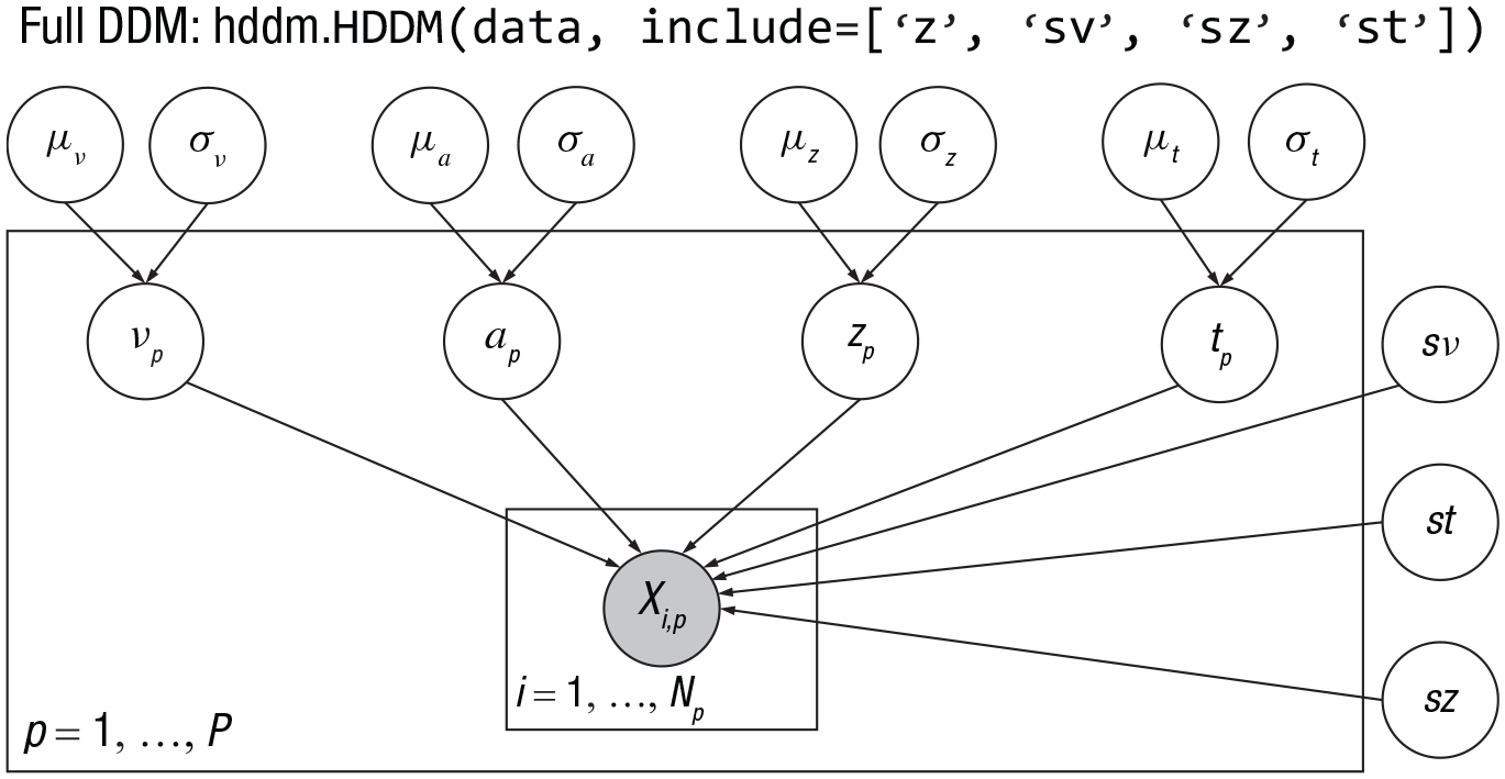
Note: The hierarchical structure of the full DDM in HDDM. The parameters inside and outside the rectangle are subject and population level parameters, respectively. $p / i$ are the indices of participants ( $p = 1, 2, \dots, P$ ) and trials ( $i = 1, 2, \dots . N$ ), where $x_{i, p}$ is the data (choice/response time) of the ith trial in the pth subject.

Consequently, there are a total of 11 population-level parameters. At the subject level, subjects have their own estimate of the parameter of a, v, t, z, leading to a total of $4 \times p$ subject-level parameters. Thus, in the full DDM, the number of parameters is 11 plus $4 \times p$ .

HDDM provides two types of priors: weakly informative priors and noninformative priors. By default, dockerHDDM uses weakly informative priors as summarized in the table below (Wiecki et al., 2013). The default informative priors are suitable for most perceptual tasks. However, for tasks with longer response times, it is recommended to use noninformative priors. In this case, one has to set the parameter `informative=False` when defining the model, for example, `m = hddm.HDDM(data, informative=False)`.

DDM parameters’ informative prior
$m_{v} ~ N (2, 3)$	$σ_{v} ~ ℋ N (2)$	$v_{p} ~ N (μ_{v}, σ_{v}^{2})$
$m_{a} ~ G (1.5, 0.75)$	$σ_{a} ~ ℋ N (2)$	$a_{p} ~ G (μ_{a}, σ_{a}^{2})$
$m_{z} ~ i n v l o g i t (N (0.5, 0.5))$	$σ_{z} ~ ℋ N (0.05)$	$z_{p} ~ N (μ_{z}, σ_{z}^{2})$
$m_{t} ~ G (0.4, 0.2)$	$σ_{t} ~ ℋ N (1)$	$t_{p} ~ N (μ_{t}, σ_{t}^{2})$
$s v ~ ℋ N (2)$	$s t ~ ℋ N (0.3)$	$s z ~ ℬ (1, 3)$

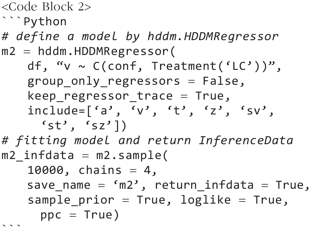
Note: Table extracted and refined from Wiecki et al. (2013). $N$ represents a normal distribution parameterized by the mean (m $μ$ ) and standard deviation ( $σ$ ). $ℋ N$ represents a half-normal distribution, which is a positive-only distribution parameterized by the standard deviation. $G$ represents a gamma distribution, parameterized by the mean (m $μ$ ) and the rate ( $σ$ ). $ℬ$ represents a beta distribution, parameterized by alpha and beta. The term $i n v l o g i t$ represents the inverse logit function also known as the logistic function.

HDDM also allows parameters to vary with variables by integrating hierarchical linear regression models (also called “linear mixed models” or “multilevel models”). Specifically, the `hddm.HDDMRegressor()` function allows any or all of the four parameters of DDM (a, v, t, z) to be modeled as a function of experimental conditions or other variables (e.g., EEG signal). In HDDM, the regression models are defined using the Python package patsy (see https://patsy.readthedocs.io/en/latest/quickstart.html), which uses the same syntax for defining regression functions as in other commonly used statistical packages. For example, in Model 2 in the main text, we used the expression `v ~ 1 + C(conf, Treatment(‘LC’))`, where the term to the left of “~” is the dependent variable and the term to the right of “~” is the regression equation. The term ‘1’ refers to the intercept, which corresponds to the variable “V_Intercept” in the output. The term “C(conf, Treatment(‘LC’))” indicates the slope coefficient, which corresponds to the variable “v_C(conf, Treatment(‘LC’))[T.HC]”. As in other hierarchical regression models, both the intercept and the slope can be estimated at the population level and the subject level (referred to as “fixed effects” and “random effects” or “varying effects,” respectively; D. J. Johnson et al., 2017; Pedersen & Frank, 2020; Wiecki et al., 2013), depending on how the model is specified. In `hddm.HDDMRegressor()`, the default is hierarchical model with random intercept but no random slope. We need to set `group_only_regressors=False` to include the random slope (as we did in Model 2).

Although both the `depends_on` argument and the `HDDMRegressor` function allow parameters to vary with discrete variables (e.g., conflict levels), there is an important difference between them. The `depends_on` argument defines the parameter split by condition. Specifically, the means of the parameters under each condition are derived from a share prior, whereas the variability of the parameters is consistent across conditions. The `HDDMRegressor` function defines the relation between parameters and condition by a linear model specification, which means the intercept and slope in the linear regression both have their own priors. In a word, `depends_on` is unable to use within-subjects effects because each subject’s condition is derived from the population prior, whereas `HDDMRegressor` allows subjects to have their own intercept, which allows for the estimation of within-subjects variation across conditions. Thus, the choice of model definition is relevant to the assumptions made about the relationship between parameters and the experimental conditions. For more details, see Wiecki et al. (2013).

Model 1 allows the drift rate to vary as a function of the conflict levels (i.e., `depends_on={‘v’: ‘conf’}` in HDDM). Specifically, Model 1 sets two drift-rate variables each for low- and high-conflict levels at both the population and individual levels, respectively. Thus, Model 1 has 12 population-level parameters: the means and standard deviations for $a$ , $t$ , and $z$ ; two means (“v_(LC)” and “v_(HC)”) and one standard deviation for $v$ ; and three intertrial variability parameters ( $s v$ / $s t$ / $s z$ ). Likewise, at the individual level, there are 5 ( $v_{L C}$ / $v_{H C}$ / $t$ / $z$ / $a$ ) × 14 (subjects) = 70 individual-level parameters. Thus, Model 1 has a total of 82 free parameters.

Note that Model 1 assumes complete independence between high and low levels of conflict within subjects. This assumption may be inappropriate because it is likely that a person who responded relatively quickly in the “LC” condition will also respond relatively quickly in the “HC” condition and vice versa. For more detailed differences between Model 1 and Model 2, see Box 3.

Model 2 was constructed to include correlations between drift rates across conflicting levels. In Model 2, we use a hierarchical regression model with `hddm.HDDMRegressor()` by using the formula `v ~ 1 + C(conf, Treatment(‘LC’))` (see Box 3). This formulation automatically assigns two free parameters, the intercept and slope, to each subject. Thus, there are $5 \times 14 = 70$ individual-level parameters in Model 2. Accordingly, Model 2 has four parameters for v: “v_Intercept” and “v_Intercept_std” are the mean and standard deviation of the intercept, and “v_C(conf)[T.HC]” and “v_C(conf)[T.HC]_std” are the mean and standard deviation of the slope. Therefore, Model 2 has 13 population-level parameters: the means and standard deviations for $a$ , $t$ , and $z$ ; the means and standard deviations of the slope and the intercept of the regression for $v$ ; and three intertrial variability parameters ( $s v$ / $s t$ / $s z$ ). Taken together, Model 2 has a total of 13 + 70 = 83 free parameters.

Model fitting

The defined HDDM model allows the MCMC algorithm to be run using the `.sample()` method for model fitting and parameter estimation. The definition and fitting of Model 2 are used here as an example (see <Code Block 2>):

To accurately estimate parameters and ensure convergence in hierarchical modeling, we set up four MCMC chains of 10,000 samples with 5,000 burn-ins (i.e., a total of 20,000 samples for each parameter). For the more detailed settings and arguments description, see “Novel Features of dockerHDDM.” With the new functionality introduced by dockerHDDM, we can calculate the log-likelihood of the model and generate posterior predictions after model fitting. Furthermore, the output of the model fitting can be converted into InferenceData, `m2_infdata`, for subsequent analyses, as described in “Novel Features of dockerHDDM.”

We emphasize that model fitting is demanding in terms of computational resources and memory. For example, in our tests with the Apple M1 chip, Intel i7-10700 CPU, and AMD Ryzen 9-5900HX, model fitting took around 2 hr to 3 hr for 10,000 samples. Consequently, fitting three models took about 6 hr to 9 hr, and memory usage ranged between 8 GB and 12 GB. In addition, if pointwise likelihood calculations (i.e., with the argument `loglike=True`) and posterior predictive data generation (i.e., with the argument `ppc=True`) are enabled, an extra 1 hr to 3 hr are needed for each model. More important, the memory consumption could escalate to 20 GB to 30 GB because pointwise likelihood and posterior predictive data generation will result in a large number of new data. See discussion for recommendations to improve efficiency.

Model diagnosis

In Bayesian inference, it is crucial to ensure the convergence of MCMC chains. With ArivZ, dockerHDDM supports both visual inspection and quantitative convergence checks (Martin et al., 2024, Chapter 10).

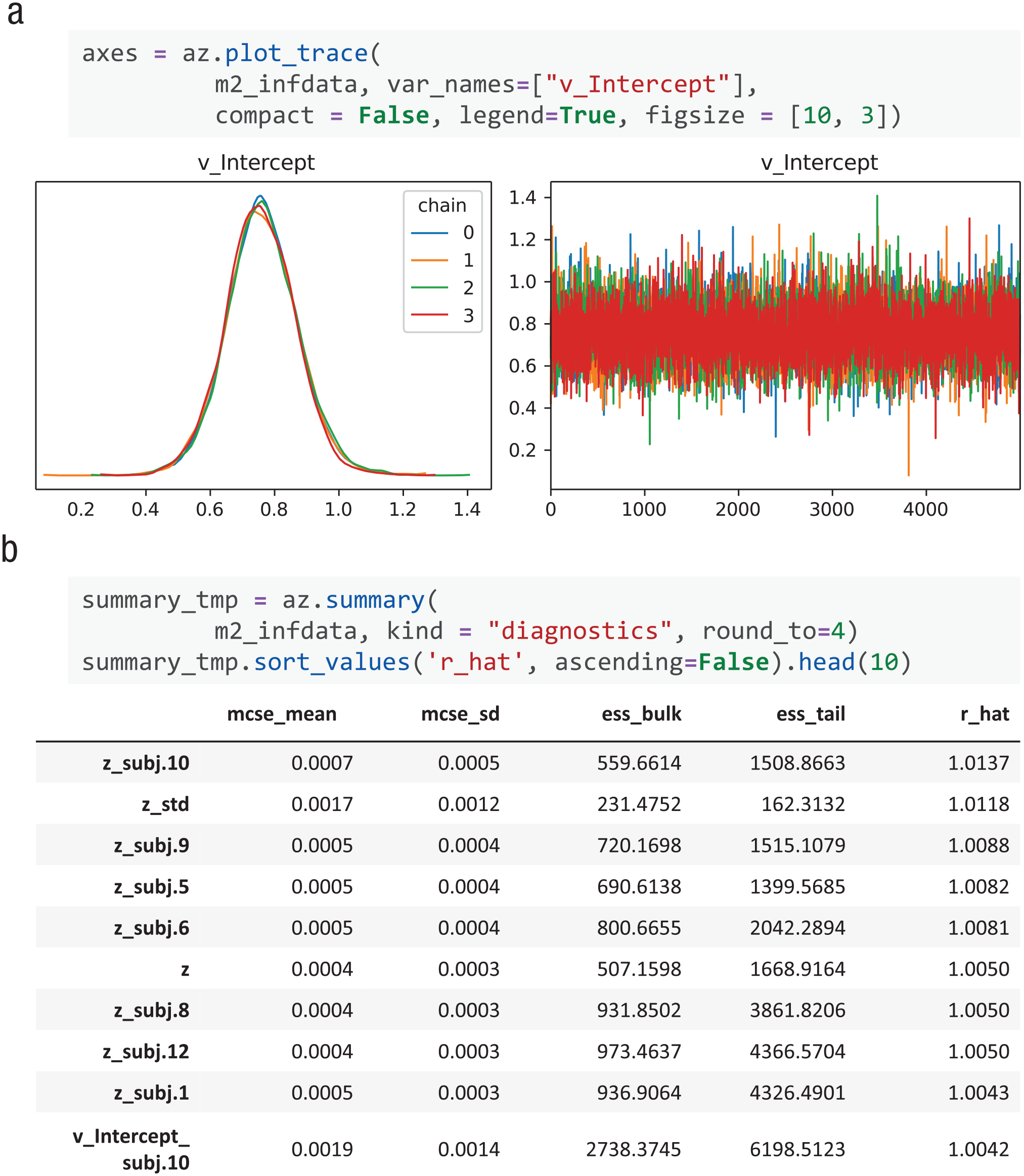
`az.plot_trace()` can be used to visualize the posterior distributions of parameters (i.e., trace plots of the MCMC, Fig. 5a).

Fig. 5.

Model diagnosis. (a) Visualization of the traces of all chains using `az.plot_trace()`, with the argument `var_names` set to focus on the parameter “v_Intercept” as an example. `compact=False` and `legend=True` ensured that the individual traces of each chain would be visible. The Markov chain Monte Carlo (MCMC) chains are valid and reliable when they fluctuate around a value and different chains are indistinguishable from each other, a scenario often referred to as a “caterpillar” shape. (b) Output of `az.summary()`, which includes the mean and standard deviation of the Monte Carlo standard error (MCSE), the effective sample sizes (bulk-ESS and tail-ESS), and $\hat{R}$ . Note that the summary data frame has been sorted by $\hat{R}$ so that we can easily compare the minimum and maximum values of $\hat{R}$ .

The Gelman-Rubin statistics ( $\hat{R}$ ), and effective sample size (ESS) provide quantitative measures (see Box 1).

`az.rhat()`computes $\hat{R}$ , which should be close to 1 for good convergence; values below 1.01 are typically recommended (Gelman & Rubin, 1992).

`az.ess()` calculates ESS, a measure of the precision of posterior estimates. If the ESS-bulk is over 400 (see Box 1), the distribution’s center is well resolved, and we should ensure high ESS across all regions of the parameter space (Martin et al., 2024; Vehtari et al., 2021).

The latter two methods are covered by ArviZ’s `az.summary()` (Fig. 5b).

Model comparison

Upon verifying chain convergence, we proceed with model comparison to identify the best-fitting model. The evaluation metric provided in the original HDDM is deviance information criterion (Spiegelhalter et al., 2002). We include two more methods in dockerHDDM: widely applicable information criterion (WAIC; Watanabe, 2010) and Pareto-smoothed importance sampling leave-one-out cross-validation (PSIS-LOO-CV; Vehtari et al., 2017). These methods comprehensively integrate posterior samples for model comparison and evaluation (see Box 4).

Box 4.

Linking Deviance Information Criterion, Widely Applicable Information Criterion, and Pareto-Smoothed Importance Sampling Leave-One-Out Cross-Validation to Akaike Information Criterion

The deviance information criterion (DIC), widely applicable information criterion (WAIC), and Pareto-smoothed importance sampling leave-one-out cross-validation (PSIS-LOO-CV) are criteria founded on the concept of out-of-sample predictive accuracy, that is, the accuracy of using the fitted model to predict new data generated by the assumed data-generating process. Predictive accuracy is often encapsulated by the log predictive density (Box 1). However, the log predictive density approximated using the observed data and the posterior estimates of parameters is biased, and an adjustment is required to correct the bias. Thus, the key difference between DIC, WAIC, and PSIS-LOO-CV lies in the difference between the two terms of log predicted density and corrected bias (see the table below).

	Predictive accuracy	Adjustment	Formula
AIC	$l o g p (y \| {\hat{θ}}_{m l e})$	k	$- 2 (l o g p (y \| {\hat{θ}}_{mle}) - k)$
DIC	$l o g p (y \| \hat{θ_{B a y e s}})$	$P_{D I C}$	$- 2 (l o g p (y \| \hat{θ_{B a y e s}}) - P_{D I C})$
WAIC	$\hat{l p d}$	${\hat{p}}_{W A I C}$	$- 2 (\hat{l p d} - {\hat{p}}_{W A I C})$
PSIS-LOO-CV	${\hat{e l p d}}_{p s i s - l o o}$		$- 2 e l p d_{p s i s - l o o}$

Note: $\hat{l p d}$ = computed log pointwise predictive density, see Glossary for details; ${\hat{e l p d}}_{p s i s - l o o}$ = expected log pointwise predictive density for a new dataset based on PSIS-LOO method; k = the count of model parameters; $P_{D I C}$ = the DIC’s adjustment for the effective number of parameters (Spiegelhalter et al., 2002); ${\hat{p}}_{W A I C}$ = the WAIC’s approach to adjusting the effective number of parameters (Watanabe, 2010). DIC = deviance information criterion; WAIC = widely applicable information criterion; PSIS-LOO-CV = Pareto-smoothed importance sampling leave-one-out cross-validation.

DIC uses the Bayesian posterior means for estimating log predictive density and includes an adjustment based on the effective number of parameters ( $P_{DIC}$ ). It is particularly suited for hierarchical models, offering an improved estimate of predictive density (Spiegelhalter et al., 2002).

WAIC further refines DIC, evaluating the log predictive density across the entire posterior and correcting bias via the variability of log predictive density ( ${\hat{p}}_{WAIC}$ ). This adjustment is crucial for measuring model robustness and guarding against overfitting (Watanabe, 2010). Both DIC and WAIC rely on estimating the effective number of parameters, but DIC assumes a Gaussian distribution for the likelihood, which simplifies the calculation (Lunn et al., 2012). In contrast, WAIC does not rely on this strict assumption and uses the full posterior distribution, offering greater flexibility and accuracy but at a higher computational complexity (Gelman et al., 2014).

PSIS-LOO-CV estimates the predictive density by simulating the leave-one-out cross-validation, which by definition is the out-of-sample predictive accuracy, so bias correction is no longer needed for PSIS-LOO-CV. For more details on these three indices, see Gelman et al. (2014) and Vehtari et al. (2017).

For the demonstration, we compared three models across all three evaluation metrics (lower value is better).⁵ As shown in Table 5, Model 2 exhibits the lowest values on all three metrics, indicating it is the best model. The results of model comparison revealed that Models 1 and 2 are much better than the baseline Model 0, suggesting that experimental conflict conditions have a substantial effect on drift rates. Moreover, Model 2 is slightly better than Model 1, suggesting that regression model may suit the data better. Nevertheless, the similarities between Model 1 and Model 2 suggest that both models fit the data adequately in this case.

Table 5.

Model Comparison With Different Criteria

Rank^a	DIC	PSIS-LOO-CV	WAIC
1	m2 (10,654.89)	m2 (10,646.25)	m2 (10,646.20)
2	m1 (10,655.24)	m1 (10,647.21)	m1 (10,647.15)
3	m0 (10,835.24)	m0 (10,824.93)	m0 (10,824.89)

Note: DIC = deviance information criterion; PSIS-LOO-CV = Pareto-smoothed importance sampling leave-one-out cross-validation; WAIC widely applicable information criterion; m0 = Model 0; m1 = Model 1; m2 = Model 2.

Rank is ranging from the best model to the worst.

Note that WAIC and PSIS-LOO-CV require the pointwise log-likelihood of each data point given a posterior sample of parameters, which must be computed using the likelihood function and posterior trace (see Box 1). This variable is not directly provided in the HDDM object and must be customized to be calculated via the likelihood function and posterior trace.

In dockerHDDM, the pointwise log-likelihood can be computed at the sampling and fitting stage, via `m.sample(. . . , retutn_infdata = True, loglike = True)` (see <Code Block 2>), or after the model has been sampled and fitted, by `m.to_infdata(loglike = True)`. Both ways return InferenceData, allowing users to immediately compute WAIC and PSIS-LOO-CV. After that, the evaluation metrics for each model’s InferenceData are available using ArviZ’s `compare` method (see <Code Block 3>), which returns the results of WAIC for the argument `ic=“waic”` or PSIS-LOO-CV for `ic=“loo”`.

Finally, we note that the model-comparison metrics allow only a relative ranking of alternatives. To assess the absolute goodness of fit of the model, we recommend performing the PPC, as discussed in the next section, alongside the diagnostic information provided by LOO and WAIC (see Martin et al., 2024, Chapter 5; Vehtari et al., 2017).

PPC

In addition to model comparison, which assesses relative performance, the PPC evaluates how well predictive data generated from posterior samples of parameters align with the actual data. PPC is crucial because model comparison evaluates only the “least worst” model, but this model may not necessarily account for the data very well (see Martin et al., 2024, Chapter 5).

ArviZ offers convenient visualization tools for inspecting PPC (Kumar et al., 2019). The function `az.plot_ppc()` is helpful to visualize PPC at the individual or condition level (Fig. 6). In the demonstration, the synthetic data from Model 2 match more closely the actual data compared with the baseline Model 0, and this difference becomes apparent when examining PPC at the individual level (Fig. 6a) and condition level (Fig. 6b). Other approaches for PPCs can be used to quantify accordance between data and model across quantiles of the response time (RT) distribution, for example, using Bayesian predictive versions of quantile probability plots (Frank et al., 2015; Ging-Jehli et al., 2021), and example code in HDDM is available on request.

Fig. 6.

Posterior predictive check plot `az.plot_ppc()` for Model 0 “m0” and Model 2 “m2.” Solid black lines are the density plot of the observed response time (RT) data; blue lines are the posterior predictive samples; each line represents the predicted RT distribution based on one posterior predictive sample; yellow dashed lines represent the mean of all predicted RT distributions across all posterior predictive samples. (a) Results of the comparison between the two models (m0 vs. m2) at the individual level (Subjects 3 and 11 as an example). (b) Results of the comparison at the condition level (i.e., “LC” represents lower conflict, and “HC” represents higher conflict). All plots in the left column are for m0, and all plots in the right column are for m2. Note that the argument `coords` specifies the posterior-predictive-check level (individual or group level) that should be preprocessed before plotting. `num_pp_samples` is used to set the number of predictive data required for plotting.

Statistical inference

A final step in Bayesian modeling is to draw statistical inferences from the posterior parameter distributions in the best-fitting model. In our example, we test the hypothesis of whether drift rates significantly differ between HC and LC conditions based on Model2 (“m2” in the Notebook). This hypothesis is tested using the posterior samples of the regression coefficient in “m2,” which has a variable name “v_C(conf, Treatment(‘LC’))[T.HC]”.

Note that there are several acceptable methods for Bayesian hypothesis testing, such as BFs (Boehm et al., 2023; Wagenmakers et al., 2010), maximum a posteriori based p value (Mills, 2018), directional probabilities (Makowski et al., 2019), and the full Bayesian significance test (Kelter, 2022). In cognitive science and psychology, although BFs are often advocated as a Bayesian alternative to frequentist p values (Kelter, 2021; van de Schoot et al., 2017; Wagenmakers et al., 2010), debate remains about which Bayesian measures should be used in which settings of scientific hypothesis testing (Kelter, 2023; Makowski et al., 2019). Therefore, it is useful to consider various Bayesian hypothesis-testing methods depending on the study objectives and design (Kelter, 2023; Kruschke, 2021; Makowski et al., 2019).

Here, we demonstrate Bayesian inference using an approach that combines the approach combining highest density interval (HDI) and the region of practical equivalence (ROPE; Kruschke, 2018; see Box 1). In addition, we provide methods for calculating BFs in the Appendix.

We define a ROPE of [–0.2, 0.2] to represent values practically equivalent to zero⁶ and use the `plot_posterior()` function from ArviZ to implement the ROPE test. By comparing the 95% HDI of the regression coefficient to this ROPE, we find that the HDI falls completely outside the ROPE (Fig. 7a), suggesting that the drift rate is higher in the LC condition than the HC condition (Fig. 7b).

Fig. 7.

(a) Statistical inference of parameters. The high-density interval (HDI; black line and texts) is compared with the region of practical equivalence (ROPE; red line and text). `var_names` argument can be used to select both group-level and individual-level parameters for analysis. `hdi_prob` argument specifies the probability of the HDI, typically set at 0.95 to correspond to a 95% credible interval. `rope` defines the limitations of ROPE, which is a range considered to be equivalent to the null hypothesis or a reference value for the parameter. The results show no overlap between the 95% HDI and the ROPE, indicating that the parameter is credibly different from zero. (b) Violin plot of parameter posteriors at two conflict levels. The black line is the 95% HDI, and the white dot is the mean. The drift rate is lower in high-conflict (HC) conditions than in low-conflict (LC) conditions.

Therefore, considering the results from various aspects (model comparison, PPC, and posterior inference), we conclude that the model that takes into account the influence of conflict level on drift rate performs the best. Moreover, HC affects the cognitive process of decision-making by impeding the speed of evidence accumulation.

Discussion

In this tutorial, we focus on an easy-to-use computational environment for HDDM, including installation of the tool, its features, and case applications. Although some conceptual discussions have been addressed in other articles (Boag et al., 2024; Shinn et al., 2020; Voss et al., 2013), we nevertheless discuss some relevant issues below.

Why use dockerHDDM among tools?

Inference for the DDM can be implemented via multiple software/packages, such as fast-DM (Voss & Voss, 2007), flexDDM (LaFollette et al., 2024), rtdists (Singmann et al., 2022), EZ-DDM (Wagenmakers et al., 2007), and pyDDM (Shinn et al., 2020). For more details on tool and algorithm comparisons, see Shinn et al. (2020). Although all the above tools are estimated in a frequency framework and fit data at the individual-participant level, HDDM takes the Bayesian approach and estimates model parameters at both the individual and group levels (i.e., the hierarchical-model or multilevel-model approach; see Wiecki et al., 2013). Tools that also allow the Bayesian hierarchical modeling approach of DDM include brms based on RStan (Henrich et al., 2023), the Wiener module in JAGS (Wabersich & Vandekerckhove, 2014), EMC2 (Stevenson et al., 2024), and hBayesDM (Ahn et al., 2017). For comparison between these tools and HDDM, see Table 6.

Table 6.

Tools Comparison for Modeling Hierarchical DDM

	(docker)HDDM	brms/RStan/hBayesDM	JAGS	EMC2
Language	Python	R	R	R
MCMC Algorithm	Metropolis-Hastings	NUTS	Gibbs sampling	Particle Metropolis
Support models	DDM, full DDM, RLDDM, collapsing boundary variants, etc.	DDM, full DDM	DDM	DDM, LBA, RDM, etc.
Custom prior	No	Yes	Yes	Yes
Linear mixed extension	Yes	Yes	Yes	Yes
Likelihood-free	Yes	No	No	No

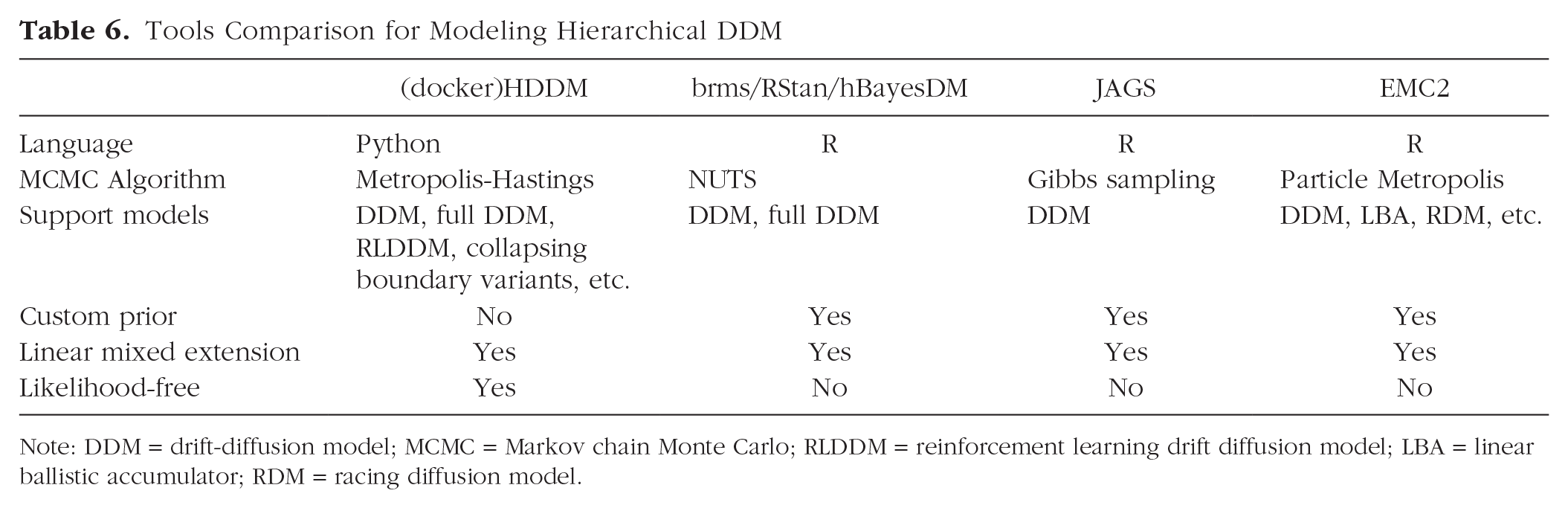
Note: DDM = drift-diffusion model; MCMC = Markov chain Monte Carlo; RLDDM = reinforcement learning drift diffusion model; LBA = linear ballistic accumulator; RDM = racing diffusion model.

HDDM stands out for its ease of use, enabling users to construct and fit basic models with just a few lines of code. It facilitates the definition of complex mixed-effects models without the need for prior specifications, making it more accessible for beginners. Although brms and EMC2 also define mixed-effects models well, they necessitate users to manually define prior distributions for random effects and covariance structures. In addition, RStan and JAGS require expertise in linear model reparameterization. The absence of this expertise may result in model-fitting failures or biased estimates. On the other hand, the simplicity of HDDM comes at the cost of flexibility because it restricts users to the default priors (see Box 3) and does not allow for customization. However, the weakly informative prior implemented in HDDM was based on previous meta-analyses of published results (Matzke & Wagenmakers, 2009) and applicable to typical cognitive experiments.

Another advantage of HDDM is its support for diverse accumulation models, including models with collapsing boundaries and those integrated with reinforcement learning, called “RLDDM” (Fengler et al., 2022; Pedersen & Frank, 2020; Pedersen et al., 2017). In addition, the latest version of HDDM provides many likelihood-free models, broadening its applications. For instance, its integration with neural networks, such as the LANs (likelihood approximation networks; Fengler et al., 2021), has greatly enhanced the efficiency of model design and development.

A notable limitation of dockerHDDM is its lack of integration with the most advanced parameter-estimation techniques. For instance, its successors, HSSM and EMC2, have begun incorporating advanced MCMC methods. Moreover, innovative neural-network approaches, such as LANs (Fengler et al., 2021), MNLE (Boelts et al., 2022), and Bayesflow (Radev et al., 2022), have the potential to significantly enhance these estimation procedures. However, the mastery of these cutting-edge techniques requires a higher level of expertise to prevent misuse.

Consequently, we propose that the mission of dockerHDDM should be to streamline operations and lower the barrier to entry, facilitating analogical learning and, ultimately, preparing users for the transition to the more sophisticated methods.

Whether to include parameters’ intertrial variability?

As a demonstration, we used the seven-parameter full DDM. If a user wishes to fit only the four-parameter model, the unnecessary parameters can be removed from the include argument, for example, `include=[‘a’, ‘v’, ‘t’, ‘z’]`. In contrast, the full model, which integrates trial-by-trial variability, is known for its robustness in fitting various data sets and accommodating extreme response times, including fast and slow errors (Schubert et al., 2017). However, Lerche and Voss (2016) argued that excluding trial-by-trial parameters can enhance the fit and recovery of fundamental parameters.

Consequently, the choice to include trial-by-trial variability requires a delicate balance between the prediction and complexity of the model and the specific requirements of the data. Given the extensive data requirements for inferring across-trial variability, our stance is to cautiously include across-trial variability in the model for a more robust fit and more precise inference of the basic parameters (see similar discussion in Boag et al., 2024). For instance, because the variability of the nondecision time tends to be easily recovered (e.g., the result of the parameter recovery in Appendix Figure S2), it may be prudent to include only this parameter but not the other variability parameters by default. Nevertheless, when the data set is substantial and the research objective prioritizes the analysis of specific response-time patterns, such as fast or slow errors, the selective integration (the parameter variability of drift and start point; also see Table 1) of these parameters may be warranted. We recommend reading the work by Boehm et al. (2018), which offers expert advice and recommendations on estimating across-trial variability parameters.

Data quantity and quality for fitting the DDM

Both the number of subjects and the number of trials should be considered. Because of the hierarchical nature of the model, hierarchical models typically require fewer trials than nonhierarchical models (Alexandrowicz & Gula, 2020; Wiecki et al., 2013). In general, 12 subjects are sufficient to obtain stable results (Wiecki et al., 2013), but we recommend collecting data from more than 20 subjects for a more robust fit. However, the number of sufficient trials varies depending on the parameters of interest. For the basic four-parameter model, the number of trials has a small effect on parameter estimates (Alexandrowicz & Gula, 2020). Twenty trials appears to be the minimum standard, and more than 50 trials tend to produce robust results (Wiecki et al., 2013). Estimates of $t$ and $z$ tend to be superior to those of $a$ and $v$ . To obtain more accurate estimates of $v$ , a number of trials greater than 100 is recommended (Alexandrowicz & Gula, 2020). For parameters such as $s v$ , $s t$ , and $s z$ , a large number of trials are required for estimation, preferably more than 120 trials (Wiecki et al., 2013). Recent discourse has emphasized that the determination of the number of subjects and trials should be aligned with considerations of experimental design, desired target effects, and parameter recovery simulations (Boag et al., 2024). For further empirical guidelines, see Boehm et al. (2018) and Lerche and Voss (2017).

Note that parameter estimation can be affected by extreme values, such as very fast response times. HDDM addresses this issue by assuming a mixture model in which a proportion of the response times are from a uniform distribution (Ratcliff & Tuerlinckx, 2002; Wiecki et al., 2013). The proportion of response times is controlled by the parameter `p_outlier`, which is set to 0.05 by default. This approach helps mitigate the effect of extreme values and ensures a more robust parameter estimation.

Finally, it is essential to conduct PPCs to validate the model (see “PPC”). These checks help to ensure that the model is capable of accurately reproducing the observed data, thus providing confidence in the evaluation of the model and parameters.

Computational resources and tips

To achieve accurate estimates, more subjects, more trials, and often more samples are required, leading to increased demands for computational resources. This is not unique to dockerHDDM; other tools using MCMC algorithms, such as DMC and brms mentioned earlier, are also affected by these factors. In the examples provided in this article, fitting each model with 14 subjects and 3,988 trials takes 2 hr to 3 hr and requires 8 GB to 12 GB of memory. Running out of memory can cause the Jupyter kernel to suspend and restart, interrupting the process. Predictably, computational resources become a limiting factor with increasing data. To facilitate better model analysis, we offer the following tips and recommendations.

Initial testing

When initially building the model, use subset data from a small number of subjects and reduce the MCMC sample size to verify that the model definition and code are correct. Once validated, increase the data and sample sizes.

Adjust memory settings

If users experience a Jupyter kernel suspension or restart because of memory constraints, they can attempt to configure or increase virtual memory. For Windows users, it is necessary to check and remove the memory-usage limitations imposed by WSL (Windows Subsystem for Linux).

Separate execution

Model fitting, calculation of point-wise log likelihood, and generation of PPCs data can be executed separately. This approach helps prevent interrupting long-running processes because of errors and ensures that each step can be independently validated and debugged before proceeding to the next.

Notebook segmentation

Fit models into separate notebooks to reduce the resource load of loading multiple models.

Model saving

Save the fitted models and then load only the InferenceData files instead of the entire models to reduce resource usage.

Cloud deployment

Docker is easily deployed in cloud-computing environments (or use the docker image in Singularity). Use your institution’s computing services or rent cloud computing services to handle larger data sets.

Summary

In this article, we introduce dockerHDDM, a user-friendly, out-of-the-box, and one-stop Docker image for implementing HDDM analysis within a modern Bayesian hierarchical workflow. Our dockerHDDM has three major advantages: (a) It leverages Docker to solve compatibility issues and simplify the installation process, (b) it ensures broad support across different machines equipped with either Intel or Apple chips, and (c) it integrates state-of-the-art Bayesian modeling practices with ArviZ, facilitating a more principled Bayesian workflow. We also provide a step-by-step video tutorial on how to use dockerHDDM.

Although we have provided a step-by-step guide to using dockerHDDM, it is unfortunately not possible to provide a comprehensive introduction to computational modeling. Given the extensive knowledge required for principled computational modeling, we recommend readers refer to the materials in Box 5 for a deeper understanding of the DDM family, computational modeling, hierarchical models, and Bayesian modeling. We expect that dockerHDDM and this detailed tutorial will reduce the technical burden and help readers get started with computational modeling. Ultimately, we hope that this tool and the computational-modeling concepts presented in the tutorial will promote the computational reproducibility of drift-diffusion modeling for users of all levels of computational expertise.

Box 5.

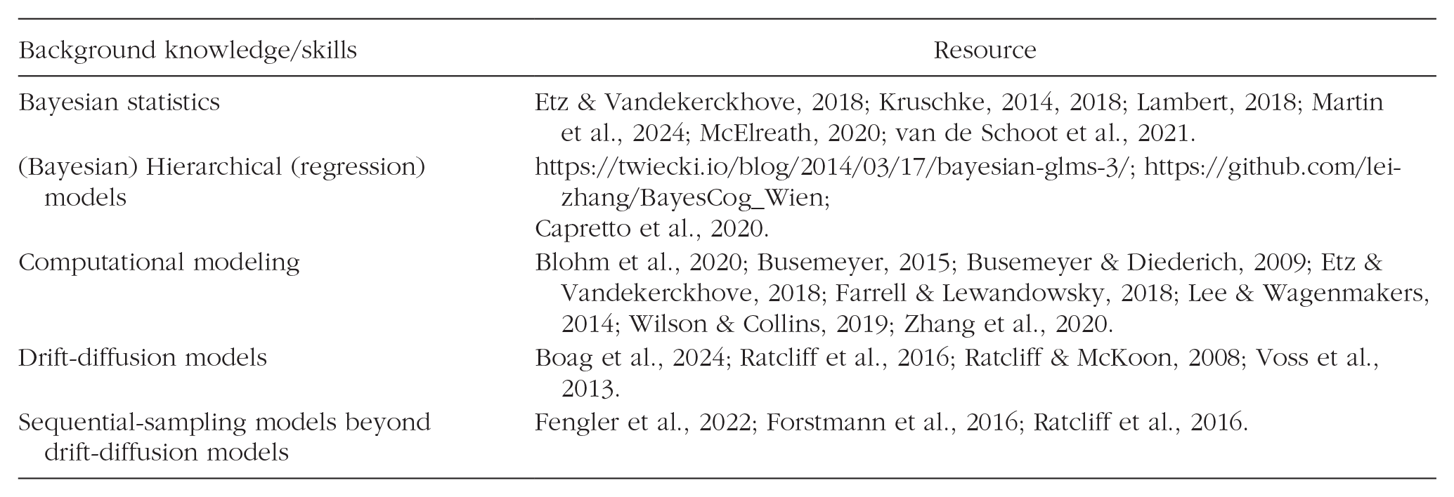
Recommendation for Further Reading

A full understanding of how Bayesian hierarchical drift-diffusion modeling works requires not only basic knowledge of drift-diffusion modeling but also knowledge of Python programming, Bayesian statistics, and hierarchical regression models. This background knowledge is generally not part of the coursework in psychology or neuroscience education, although the situation has been changing in recent years. We recommend the following resources to quickly catch up and avoid misuse or abuse of hierarchical drift-diffusion modeling.

Background knowledge/skills	Resource
Bayesian statistics	Etz & Vandekerckhove, 2018; Kruschke, 2014, 2018; Lambert, 2018; Martin et al., 2024; McElreath, 2020; van de Schoot et al., 2021.
(Bayesian) Hierarchical (regression) models	https://twiecki.io/blog/2014/03/17/bayesian-glms-3/; https://github.com/lei-zhang/BayesCog_Wien;Capretto et al., 2020.
Computational modeling	Blohm et al., 2020; Busemeyer, 2015; Busemeyer & Diederich, 2009; Etz & Vandekerckhove, 2018; Farrell & Lewandowsky, 2018; Lee & Wagenmakers, 2014; Wilson & Collins, 2019; Zhang et al., 2020.
Drift-diffusion models	Boag et al., 2024; Ratcliff et al., 2016; Ratcliff & McKoon, 2008; Voss et al., 2013.
Sequential-sampling models beyond drift-diffusion models	Fengler et al., 2022; Forstmann et al., 2016; Ratcliff et al., 2016.

Footnotes

Appendix

Acknowledgements

Thanks to HDDM (Wiecki et al., 2013; Fengler et al., 2021; Fengler et al., 2022) and ArviZ (Kumar et al., 2019) for the open resource. We thank Dr. Mads Lund Pedersen for his open dockerfile, which insipre the current project. We also thank the netizens for their time in testing and valuable feedback, which allows us to continuously improve the tools and tutorials. We appreciate the help of Dr. Yuan Rui in the early stage of docker image development.

Transparency

Action Editor: Rogier Kievit

Editor: David A. Sbarra

Author Contributions

Wanke Pan: Software; Validation; Visualization; Writing – original draft.

Haiyang Geng: Conceptualization; Writing – original draft; Writing – review & editing.

Lei Zhang: Conceptualization; Writing – original draft; Writing – review & editing.

Alexander Fengler: Writing – original draft; Writing – review & editing.

Michael J. Frank: Writing – original draft; Writing – review & editing.

Ru-Yuan Zhang: Conceptualization; Funding acquisition; Supervision; Writing – original draft; Writing – review & editing.

Hu Chuan-Peng: Conceptualization; Funding acquisition; Software; Supervision; Writing – original draft; Writing – review & editing.

ORCID iDs

Wanke Pan

Haiyang Geng

Lei Zhang

Ru-Yuan Zhang

Hu Chuan-Peng

Notes

References

Ahn

W.-Y.

Haines

Zhang

(2017). Revealing neurocomputational mechanisms of reinforcement learning and decision-making with the hBayesDM package. Computational Psychiatry, 1, 24–57. https://doi.org/10.1162/cpsy_a_00002

Alexandrowicz

R. W.

Gula

(2020). Comparing eight parameter estimation methods for the Ratcliff diffusion model using free software. Frontiers in Psychology, 11, Article 484737. https://doi.org/10.3389/fpsyg.2020.484737

Annis

Miller

B. J.

Palmeri

T. J.

(2017). Bayesian inference with stan: A tutorial on adding custom distributions. Behavior Research Methods, 49(3), 863–886. https://doi.org/10.3758/s13428-016-0746-9

Blohm

Kording

K. P.

Schrater

P. R.

(2020). A how-to-model guide for neuroscience. Eneuro, 7(1), Article ENEURO.352-19.2019. https://doi.org/10.1523/ENEURO.0352-19.2019

Boag

R. J.

Innes

Stevenson

Bahg

Busemeyer

J. R.

Cox

G. E.

Donkin

Frank

Hawkins

Heathcote

Hedge

Lerche

Lilburn

Logan

G. D.

Matzke

Miletic

Osth

A. F.

Palmeri

Sederberg

P. B.

. . . Forstmann

(2024). An expert guide to planning experimental tasks for evidence accumulation modelling. PsyArXiv. https://doi.org/10.31234/osf.io/snqgp

Boehm

Annis

Frank

M. J.

Hawkins

G. E.

Heathcote

Kellen

Krypotos

A. M.

Lerche

Logan

G. D.

Palmeri

T. J.

van Ravenzwaaij

Servant

Singmann

Starns

J. J.

Voss

Wiecki

T. V.

Matzke

Wagenmakers

E. J.

(2018). Estimating across-trial variability parameters of the Diffusion Decision Model: Expert advice and recommendations. Journal of Mathematical Psychology, 87, 46–75. https://doi.org/10.1016/j.jmp.2018.09.004

Boehm

Evans

N. J.

Gronau

Q. F.

Matzke

Wagenmakers

E.-J.

Heathcote

A. J.

(2023). Inclusion Bayes factors for mixed hierarchical diffusion decision models. Psychological Methods, 29, 625–655. https://doi.org/10.1037/met0000582

Boelts

Lueckmann

J.-M.

Gao

Macke

J. H.

(2022). Flexible and efficient simulation-based inference for models of decision-making. eLife, 11, Article e77220. https://doi.org/10.7554/eLife.77220

Busemeyer

J. R.

(Ed.). (2015). The Oxford handbook of computational and mathematical psychology. Oxford University Press.

10.

Busemeyer

J. R.

Diederich

(2009). Cognitive modeling. Sage.

11.

Capretto

Piho

Kumar

Westfall

Yarkoni

Martin

O. A.

(2020). Bambi: A simple interface for fitting Bayesian linear models in python. arXiv. https://doi.org/10.48550/ARXIV.2012.10754

12.

Cavanagh

J. F.

Wiecki

T. V.

Cohen

M. X.

Figueroa

C. M.

Samanta

Sherman

S. J.

Frank

M. J.

(2011). Subthalamic nucleus stimulation reverses mediofrontal influence over decision threshold. Nature Neuroscience, 14(11), 1462–1467. https://doi.org/10.1038/nn.2925

13.

Chandrasekaran

Peixoto

Newsome

W. T.

Shenoy

K. V.

(2017). Laminar differences in decision-related neural activity in dorsal premotor cortex. Nature Communications, 8(1), Article 614. https://doi.org/10.1038/s41467-017-00715-0

14.

Desai

Krajbich

(2022). Decomposing preferences into predispositions and evaluations. Journal of Experimental Psychology-General, 151(8), 1883–1903. https://doi.org/10.1037/xge0001162

15.

Dienes

(2021). Obtaining evidence for no effect. Collabra: Psychology, 7(1), Article 28202. https://doi.org/10.1525/collabra.28202

16.

Donkin

Brown

S. D.

(2018). Response times and decision-making. In Wixted

J. T.

(Ed.), Stevens’ handbook of experimental psychology and cognitive neuroscience (pp. 1–33). John Wiley & Sons. https://doi.org/10.1002/9781119170174.epcn509

17.

Etz

Chávez de la Peña

A. F.

Baroja

Medriano

Vandekerckhove

(2024). The HDI + ROPE decision rule is logically incoherent but we can fix it. Psychological Methods. Advance online publication. https://doi.org/10.1037/met0000660

18.

Etz

Vandekerckhove

(2018). Introduction to Bayesian inference for psychology. Psychonomic Bulletin & Review, 25(1), 5–34. https://doi.org/10.3758/s13423-017-1262-3

19.

Evans

N. J.

Wagenmakers

E.-J.

(2020). Evidence accumulation models: Current limitations and future directions. The Quantitative Methods for Psychology, 16(2), 73–90. https://doi.org/10.20982/tqmp.16.2.p073

20.

Farrell

Lewandowsky

(2018). Computational modeling of cognition and behavior. Cambridge University Press. https://doi.org/10.1017/CBO9781316272503

21.

Fengler

Bera

Pedersen

M. L.

Frank

M. J.

(2022). Beyond drift diffusion models: Fitting a broad class of decision and reinforcement learning models with HDDM. Journal of Cognitive Neuroscience, 34(10), 1780–1805. https://doi.org/10.1162/jocn_a_01902

22.

Fengler

Govindarajan

L. N.

Chen

Frank

M. J.

(2021). Likelihood approximation networks (LANs) for fast inference of simulation models in cognitive neuroscience. eLife, 10, Article e65074. https://doi.org/10.7554/eLife.65074

23.

Forstmann

B. U.

Ratcliff

Wagenmakers

E.-J.

(2016). Sequential sampling models in cognitive neuroscience: Advantages, applications, and extensions. Annual Review of Psychology, 67(1), 641–666. https://doi.org/10.1146/annurev-psych-122414-033645

24.

Frank

M. J.

Gagne

Nyhus

Masters

Wiecki

T. V.

Cavanagh

J. F.

Badre

(2015). fMRI and EEG predictors of dynamic decision parameters during human reinforcement learning. The Journal of Neuroscience, 35(2), 485–494. https://doi.org/10.1523/JNEUROSCI.2036-14.2015

25.

Gelman

Hwang

Vehtari

(2014). Understanding predictive information criteria for Bayesian models. Statistics and Computing, 24(6), 997–1016. https://doi.org/10.1007/s11222-013-9416-2

26.

Gelman

Rubin

D. B.

(1992). Inference from iterative simulation using multiple sequences. Statistical Science, 7(4), 457–472.

27.

Gelman

Vehtari

Simpson

Margossian

C. C.

Carpenter

Yao

Kennedy

Gabry

Bürkner

P.-C.

Modrák

(2020). Bayesian workflow. arXiv. https://doi.org/10.48550/arXiv.2011.01808

28.

Ging-Jehli

N. R.

Ratcliff

Arnold

L. E.

(2021). Improving neurocognitive testing using computational psychiatry—A systematic review for ADHD. Psychological Bulletin, 147(2), 169–231. https://doi.org/10.1037/bul0000319

29.

Hedge

Powell

Bompas

Vivian-Griffiths

Sumner

(2018). Low and variable correlation between reaction time costs and accuracy costs explained by accumulation models: Meta-analysis and simulations. Psychological Bulletin, 144(11), 1200–1227. https://doi.org/10.1037/bul0000164

30.

Henrich

Hartmann

Pratz

Voss

Klauer

K. C.

(2023). The seven-parameter diffusion model: An implementation in stan for Bayesian analyses. Behavior Research Methods, 56, 3102–3116. https://doi.org/10.3758/s13428-023-02179-1

31.

Herz

D. M.

Tan

Brittain

J.-S.

Fischer

Cheeran

Green

A. L.

Fitzgerald

Aziz

T. Z.

Ashkan

Little

Foltynie

Limousin

Zrinzo

Bogacz

Brown

(2017). Distinct mechanisms mediate speed-accuracy adjustments in cortico-subthalamic networks. eLife, 6, Article e21481. https://doi.org/10.7554/eLife.21481

32.

Hoyer

Hamman

(2017). xarray: N-D labeled arrays and datasets in python. Journal of Open Research Software, 5(1), 10. https://doi.org/10.5334/jors.148

33.

C.-P.

Lan

Macrae

C. N.

Sui

(2020). Good me bad me: Prioritization of the good-self during perceptual decision-making. Collabra: Psychology, 6(1), Article 20. https://doi.org/10.1525/collabra.301

34.

Johnson

A. A.

Ott

M. Q.

Dogucu

(2022). Bayes rules! An introduction to applied Bayesian modeling. Chapman and Hall/CRC. https://www.bayesrulesbook.com/

35.

Johnson

D. J.

Hopwood

C. J.

Cesario

Pleskac

T. J.

(2017). Advancing research on cognitive processes in social and personality psychology: A hierarchical drift diffusion model primer. Social Psychological and Personality Science, 8(4), 413–423. https://doi.org/10.1177/1948550617703174

36.

Kass

R. E.

Raftery

A. E.

(1995). Bayes factors. Journal of the American Statistical Association, 90(430), 773–795. https://doi.org/10.1080/01621459.1995.10476572

37.

Kelter

(2021). Bayesian model selection in the M-open setting—Approximate posterior inference and subsampling for efficient large-scale leave-one-out cross-validation via the difference estimator. Journal of Mathematical Psychology, 100, Article 102474. https://doi.org/10.1016/j.jmp.2020.102474

38.

Kelter

(2022). fbst: An R package for the full Bayesian significance test for testing a sharp null hypothesis against its alternative via the e value. Behavior Research Methods, 54(3), 1114–1130. https://doi.org/10.3758/s13428-021-01613-6

39.

Kelter

(2023). How to choose between different Bayesian posterior indices for hypothesis testing in practice. Multivariate Behavioral Research, 58(1), 160–188. https://doi.org/10.1080/00273171.2021.1967716

40.

Kruschke

J. K.

(2014). Doing Bayesian data analysis: A tutorial with R, JAGS, and Stan. Academic Press.

41.

Kruschke

J. K.

(2018). Rejecting or accepting parameter values in Bayesian estimation. Advances in Methods and Practices in Psychological Science, 1(2), 270–280. https://doi.org/10.1177/2515245918771304

42.

Kruschke

J. K.

(2021). Bayesian analysis reporting guidelines. Nature Human Behaviour, 5(10), Article 10. https://doi.org/10.1038/s41562-021-01177-7

43.

Kumar

Carroll

Hartikainen

Martín

O. A.

(2019). ArviZ: A unified library for exploratory analysis of Bayesian models in python. Journal of Open Source Software, 4(33), Article 1143. https://doi.org/10.21105/joss.01143

44.

Kutlikova

H. H.

Zhang

Eisenegger

van Honk

Lamm

(2023). Testosterone eliminates strategic prosocial behavior through impacting choice consistency in healthy males. Neuropsychopharmacology, 48(10), Article 10. https://doi.org/10.1038/s41386-023-01570-y

45.

LaFollette

Fan

Puccio

Demaree

H. A.

(2024). FlexDDM: A flexible decision-diffusion python package for the behavioral sciences. Proceedings of the Annual Meeting of the Cognitive Science Society, 46, 4772–4778. https://escholarship.org/uc/item/4q57r2x0

46.

Lambert

(2018). A student’s guide to Bayesian statistics. Sage.

47.

Lee

M. D.

Wagenmakers

E.-J.

(2014). Bayesian cognitive modeling: A practical course. Cambridge University Press. https://doi.org/10.1017/CBO9781139087759

48.

Lerche

Voss

(2016). Model complexity in diffusion modeling: Benefits of making the model more parsimonious. Frontiers in Psychology, 7, Article 1324. https://doi.org/10.3389/fpsyg.2016.01324

49.

Lerche

Voss

(2017). Retest reliability of the parameters of the Ratcliff diffusion model. Psychological Research, 81(3), 629–652. https://doi.org/10.1007/s00426-016-0770-5

50.

Liu

Zheng

Y.-R.

Sui

Chuan-Peng

(2023). A multiverse assessment of the reliability of the self matching task as a measurement of the self-prioritization effect. PsyArXiv. https://doi.org/10.31234/osf.io/g6uap

51.

Lunn

Jackson

Best

Thomas

Spiegelhalter

(2012). The BUGS book: A practical introduction to Bayesian analysis. Chapman and Hall/CRC. https://doi.org/10.1201/b13613

52.

Makowski

Ben-Shachar

M. S.

Chen

S. H. A.

Lüdecke

(2019). Indices of effect existence and significance in the Bayesian framework. Frontiers in Psychology, 10, Article 2767. https://doi.org/10.3389/fpsyg.2019.02767

53.

Martin

Fonnesbeck

Wiecki

(2024). Bayesian analysis with python: A practical guide to probabilistic modeling (3rd ed.). Packt.

54.

Matzke

Wagenmakers

E.-J.

(2009). Psychological interpretation of the ex-Gaussian and shifted Wald parameters: A diffusion model analysis. Psychonomic Bulletin & Review, 16(5), 798–817. https://doi.org/10.3758/PBR.16.5.798

55.

McElreath

(2020). Statistical rethinking: A Bayesian course with examples in R and Stan (2nd ed.). Taylor and Francis, CRC Press. https://www.taylorfrancis.com/books/mono/10.1201/9780429029608/statistical-rethinking-richard-mcelreath

56.

Mills

J. A.

(2018). Objective Bayesian precise hypothesis testing. University of Cincinnati.

57.

Pedersen

M. L.

Alnæs

van der Meer

Fernandez-Cabello

Berthet

Dahl

Kjelkenes

Schwarz

Thompson

W. K.

Barch

D. M.

Andreassen

O. A.

Westlye

L. T.

(2022). Computational modeling of the N-Back task in the ABCD study: Associations of drift diffusion model parameters to polygenic scores of mental disorders and cardiometabolic diseases. Biological Psychiatry: Cognitive Neuroscience and Neuroimaging, 8, 290–299. https://doi.org/10.1016/j.bpsc.2022.03.012

58.

Pedersen

M. L.

Frank

M. J.

(2020). Simultaneous hierarchical Bayesian parameter estimation for reinforcement learning and drift diffusion models: A tutorial and links to neural data. Computational Brain & Behavior, 3(4), 458–471. https://doi.org/10.1007/s42113-020-00084-w

59.

Pedersen

M. L.

Frank

M. J.

Biele

(2017). The drift diffusion model as the choice rule in reinforcement learning. Psychonomic Bulletin & Review, 24(4), 1234–1251. https://doi.org/10.3758/s13423-016-1199-y

60.

Peikert

Brandmaier

A. M.

(2021). A reproducible data analysis workflow. Quantitative and Computational Methods in Behavioral Sciences, 1, Article e3763. https://doi.org/10.5964/qcmb.3763

61.

Radev

S. T.

Mertens

U. K.

Voss

Ardizzone

Kothe

(2022). BayesFlow: Learning complex stochastic models with invertible neural networks. IEEE Transactions on Neural Networks and Learning Systems, 33(4), 1452–1466. https://doi.org/10.1109/TNNLS.2020.3042395

62.

Ratcliff

McKoon

(2008). The diffusion decision model: Theory and data for two-choice decision tasks. Neural Computation, 20(4), 873–922. https://doi.org/10.1162/neco.2008.12-06-420

63.

Ratcliff

Smith

P. L.

Brown

S. D.

McKoon

(2016). Diffusion decision model: Current issues and history. Trends in Cognitive Sciences, 20(4), 260–281. https://doi.org/10.1016/j.tics.2016.01.007

64.

Ratcliff

Tuerlinckx

(2002). Estimating parameters of the diffusion model: Approaches to dealing with contaminant reaction times and parameter variability. Psychonomic Bulletin & Review, 9(3), 438–481. https://doi.org/10.3758/bf03196302

65.

Robert

C. P.

Casella

(2004). The Metropolis—Hastings algorithm. In Robert

C. P.

Casella

(Eds.), Monte Carlo statistical methods (pp. 267–320). Springer. https://doi.org/10.1007/978-1-4757-4145-2_7

66.

Schubert

A.-L.

Hagemann

Voss

Bergmann

(2017). Evaluating the model fit of diffusion models with the root mean square error of approximation. Journal of Mathematical Psychology, 77, 29–45. https://doi.org/10.1016/j.jmp.2016.08.004

67.

Shadlen

M. N.

Shohamy

(2016). Decision making and sequential sampling from memory. Neuron, 90(5), 927–939. https://doi.org/10.1016/j.neuron.2016.04.036

68.

Sheng

Ramakrishnan

Seok

Zhao

W. J.

Thelaus

Cen

Platt

M. L.

(2020). Decomposing loss aversion from gaze allocation and pupil dilation. Proceedings of the National Academy of Sciences, USA, 117(21), 11356–11363. https://doi.org/10.1073/pnas.1919670117

69.

Shinn

Lam

N. H.

Murray

J. D.

(2020). A flexible framework for simulating and fitting generalized drift-diffusion models. eLife, 9, 1–27. https://doi.org/10.7554/elife.56938

70.

Singmann

Brown

Gretton

Heathcote

Voss

Terry

(2022). rtdists: Response time distributions (Version 0.11-5) [Computer software]. https://10.32614/CRAN.package.rtdists

71.

Spiegelhalter

D. J.

Best

N. G.

Carlin

B. P.

Van Der Linde

(2002). Bayesian measures of model complexity and fit. Journal of the Royal Statistical Society Series B: Statistical Methodology, 64(4), 583–639. https://doi.org/10.1111/1467-9868.00353

72.

Stevenson

Donzallaz

M. C.

Innes

Forstmann

Matzke

Heathcote

(2024). EMC2: An R package for cognitive models of choice. PsyArXiv. https://doi.org/10.31234/osf.io/2e4dq

73.

Tran

N.-H.

Van Maanen

Heathcote

Matzke

(2021). Systematic parameter reviews in cognitive modeling: Towards a robust and cumulative characterization of psychological processes in the diffusion decision model. Frontiers in Psychology, 11, Article 608287. https://doi.org/10.3389/fpsyg.2020.608287

74.

van de Schoot

Depaoli

King

Kramer

Märtens

Tadesse

M. G.

Vannucci

Gelman

Veen

Willemsen

(2021). Bayesian statistics and modelling. Nature Reviews Methods Primers, 1, Article 16. https://doi.org/10.1038/s43586-021-00017-2

75.

van de Schoot

Winter

S. D.

Ryan

Zondervan-Zwijnenburg

Depaoli

(2017). A systematic review of Bayesian articles in psychology: The last 25 years. Psychological Methods, 22(2), 217–239. https://doi.org/10.1037/met0000100

76.

Vehtari

Gelman

Gabry

(2017). Practical Bayesian model evaluation using leave-one-out cross-validation and WAIC. Statistics and Computing, 27(5), 1413–1432. https://doi.org/10.1007/s11222-016-9696-4

77.

Vehtari

Gelman

Simpson

Carpenter

Bürkner

P.-C.

(2021). Rank-normalization, folding, and localization: An improved R2 for assessing convergence of MCMC (with discussion). Bayesian Analysis, 16(2), 667–718. https://doi.org/10.1214/20-BA1221

78.

Voss

Nagler

Lerche

(2013). Diffusion models in experimental psychology. Experimental Psychology, 60(6), 385–402. https://doi.org/10.1027/1618-3169/a000218

79.

Voss

(2007). Fast-dm: A free program for efficient diffusion model analysis. Behavior Research Methods, 39(4), 767–775. https://doi.org/10.3758/BF03192967

80.

Wabersich

Vandekerckhove

(2014). Extending JAGS: A tutorial on adding custom distributions to JAGS (with a diffusion model example). Behavior Research Methods, 46(1), 15–28. https://doi.org/10.3758/s13428-013-0369-3

81.

Wagenmakers

E.-J.

Lodewyckx

Kuriyal

Grasman

(2010). Bayesian hypothesis testing for psychologists: A tutorial on the Savage–Dickey method. Cognitive Psychology, 60(3), 158–189. https://doi.org/10.1016/j.cogpsych.2009.12.001

82.

Wagenmakers

E.-J.

Van Der Maas

H. L. J.

Grasman

R. P. P. P

. (2007). An EZ-diffusion model for response time and accuracy. Psychonomic Bulletin & Review, 14(1), 3–22. https://doi.org/10.3758/BF03194023

83.

Watanabe

(2010). Asymptotic equivalence of Bayes cross validation and widely applicable information criterion in singular learning theory. Journal of Machine Learning Research, 11(12), 3571–3594.

84.

Wiebels

Moreau

(2021). Leveraging containers for reproducible psychological research. Advances in Methods and Practices in Psychological Science, 4(2). https://doi.org/10.1177/25152459211017853

85.

Wiecki

T. V.

Sofer

Frank

M. J.

(2013). HDDM: Hierarchical Bayesian estimation of the drift-diffusion model in python. Frontiers in Neuroinformatics, 7, Article 14. https://doi.org/10.3389/fninf.2013.00014

86.

Wilson

R. C.

Collins

A. G.

(2019). Ten simple rules for the computational modeling of behavioral data. eLife, 8, Article e49547. https://doi.org/10.7554/eLife.49547

87.

Zhang

Lengersdorff

Mikus

Glascher

Lamm

(2020). Using reinforcement learning models in social neuroscience: Frameworks, pitfalls and suggestions of best practices. Social Cognitive and Affective Neuroscience, 15(6), 695–707. https://doi.org/10.1093/scan/nsaa089

dockerHDDM: A User-Friendly Environment for Bayesian Hierarchical Drift-Diffusion Modeling

Abstract

Keywords

How to Follow This Tutorial

Glossary of Terms Used in Bayesian Modeling

Install and use dockerHDDM

Install Docker

Basic Introduction to Docker

Pull dockerHDDM image

Run dockerHDDM container

Novel Features of dockerHDDM

Example of Workflow

Example Data

Model Specification

Parameters in Hierarchical Drift-Diffusion Models

Model fitting

Model diagnosis

Model comparison

Linking Deviance Information Criterion, Widely Applicable Information Criterion, and Pareto-Smoothed Importance Sampling Leave-One-Out Cross-Validation to Akaike Information Criterion

PPC

Statistical inference

Discussion

Why use dockerHDDM among tools?

Whether to include parameters’ intertrial variability?

Data quantity and quality for fitting the DDM

Computational resources and tips

Initial testing

Adjust memory settings

Separate execution

Notebook segmentation

Model saving

Cloud deployment

Summary

Recommendation for Further Reading

Footnotes

Appendix

Acknowledgements

Transparency

ORCID iDs

Notes

References