Sage Journals: Discover world-class research

Abstract

Instructors of introductory and intermediate statistics courses often teach the use of analysis of variance (ANOVA) for the purpose of comparing more than two group means and pairwise comparison procedures (PCPs) to determine which group means differ from one another following a statistically significant ANOVA test. SPSS provides 18 PCPs. The purpose of this study was to determine which PCP has the best power and maintains Type I error control both when assumptions of equal sample size and equal variance are met and when they are violated, so as to provide a single resource for use in introductory and intermediate applied statistics courses. Testing the PCPs with simulated data revealed that only the four tests developed to be used under assumption violations adequately controlled Type I error, so we recommend using one of these procedures. Power results were similar for all four of these tests, but were slightly higher for the Games-Howell test than for the others.

Keywords

power Type I error ANOVA pairwise comparison procedures

Analysis of variance (ANOVA) designs are often taught in introductory or intermediate statistics courses in graduate programs (Aiken, West, & Millsap, 2008) and are popular in applied research (Elmore & Woehlke, 1998; Goodwin & Goodwin, 1985). ANOVA is particularly useful for both experimental and quasi-experimental research, in which the outcome of interest is commonly a group mean. When there are more than two groups in a study, ANOVA provides utility over multiple t tests because ANOVA controls for the family-wise Type I error rate. When multiple independent tests are conducted on the same data, each individual test has an inherent Type I error rate of α, but the overall family-wise Type I error rate is equal to 1 – (1 – α)^m, where m is the number of tests conducted (Field, 2013, chap. 2). For example, the family-wise Type I error rate for three tests is around .14 when the nominal α is .05, which means that at least one Type I error will be committed for a set of three tests 14% of the time.

The simplest ANOVA model, often called a one-way ANOVA, consists of one grouping independent variable with three or more levels and one continuous dependent variable. If the F statistic computed in a one-way ANOVA is statistically significant, at least one of the group means differs from another. Knowing only that one group differs from another may be helpful in a limited sense, particularly when there are a small number of groups with largely disparate means, but when the number of groups increases or the means are relatively close, more information about which groups differ is required. A popular way to determine which groups have statistically significantly different means is to conduct a pairwise comparison procedure (PCP).

PCPs operate by comparing every group mean with every other group mean in a pairwise manner, and they account for conducting multiple tests in various ways. For example, Fisher’s least significant difference (LSD) was designed to control family-wise Type I error by requiring a statistically significant F test prior to being computed (Fisher, 1935). Thus, Fisher’s LSD would be computed in error (i.e., there are no statistically significant differences to be found) only if the statistically significant result of the ANOVA itself was a Type I error. Similar logic can be applied to all PCPs: If the omnibus F test is not statistically significant, why would a researcher follow up with a pairwise test? However, groups in applied research will often differ at the population level. Consequently, the omnibus F test will often be statistically significant, and a PCP will be conducted. Additionally, most software programs will provide PCP results even if the ANOVA test is not statistically significant because most PCPs were designed as multiple comparison procedures, not as post hoc tests.

The use of PCPs is not without its criticisms. Some authors have noted theoretical concerns with the use of PCPs (e.g., Rothman, 1990), and others have noted more practical considerations (e.g., Feise, 2002). Other options for dealing with multiple comparisons also exist (e.g., taking a Bayesian approach; Gelman, Hill, & Yajima, 2012). All of these arguments and suggestions have merit; indeed, we do not recommend the blind use of PCPs. Rather, when PCPs are appropriate, we seek to provide a basis for choosing which PCP is best to use. Further, despite criticisms of and alternatives to PCPs, they continue to be used in recently published research in a wide variety of fields, such as anthropology (Gonçalves et al., 2017), sports science (Tahhan, Özdal, Vural, & Mayda, 2018), biology (Stothard et al., 2017), addictive behaviors (Andreassen, Pallesen, & Griffiths, 2017), and neurology (Goldman et al., 2017). Consequently, we feel that PCPs still warrant study.

There are 18 PCPs available in the widely used Statistical Package for the Social Sciences (SPSS, Version 24): Fisher’s (1935) LSD test, the Bonferroni method (Dunn, 1959, 1961), the Sidak (1967) test, the Student-Newman-Keuls (SNK) procedure (Keuls, 1952; Newman, 1939; Student, 1927), Tukey’s honestly significant difference (HSD) test, Tukey’s B test, the Scheffé (1953) test, Duncan’s (1955) multiple range test (MRT), Hochberg’s (1974) GT2 test, Gabriel’s (1978) test, the Waller-Duncan t test (Duncan, 1965; Waller & Duncan, 1969), Dunnett’s (1955) t test, the Ryan-Einot-Gabriel-Welsch range test (REGWQ test) and Ryan-Einot-Gabriel-Welsch F test (REGWF test; Einot & Gabriel, 1975; Ryan, 1960; Welsch, 1977), the Games-Howell test (Games & Howell, 1976), Tamhane’s (1979) T2 test, Dunnett’s (1980b) C test, and Dunnett’s (1980b) T3 test. A more thorough description of each PCP, including its computation, is available in an online supplemental document we have made available at https://osf.io/p7t2c/?view_only=ec6b0641cad546bfbf2c3c13be9156f6. The overwhelming number of PCP options necessitates some sort of guidance for introductory or intermediate statistics students. In this article, we present our results for the performance of these 18 PCPs with simulated data, in an effort to provide such guidance. Rather than being arbitrarily based on historical popularity (e.g., the frequently used Tukey’s HSD), the decision of which procedure to use should be directed by questions focused on controlling family-wise Type I error while simultaneously providing high power.

Power is the ability to detect a difference in the population when there is one. In tests comparing means, power reflects the probability of correctly identifying a difference between two group means. However, power can be quantified in several different ways for PCPs. Specifically, one can examine average power, any-pair power, or all-pairs power (Demirhan, Dolgun, Demirhan, & Dolgun, 2010; Jaccard, Becker, & Wood, 1984). Average power is the proportion of true differences detected. Any-pair power refers to the probability of correctly rejecting at least one null hypothesis in a set of comparisons and thus is analogous to the family-wise error rate (probability of incorrectly rejecting at least one null hypothesis). Last, all-pairs power is the probability of rejecting all false null hypotheses. Obviously, all-pairs power is a far stricter measure than any-pair power in most cases. In this article, we report our results for all three types of power, but give more weight to average power and any-pair power when making recommendations because of the strictness of all-pairs power.

Violating the statistical assumptions associated with computing PCPs can have adverse effects on both their power and their Type I error rate. Ordinary least squares (OLS) estimation, the most commonly used estimator for ANOVA and PCPs, has several assumptions: (a) The model is correctly specified, (b) there is no measurement error in the independent variables, and (c) the residuals are independent and identically normally distributed with a mean of 0 (B. H. Cohen, 2013, chap. 10; Pedhazur, 1997). The first two assumptions and the assumption of independence of residuals are largely a concern during research design. Further, OLS has been shown to be robust to violations of normality (Bohrnstedt & Carter, 1971; Boneau, 1960; Pedhazur, 1997). Indeed, “non-normality has only minor consequences in situations represented by most research applications” (Hopkins & Weeks, 1990, p. 719). Therefore, we focused our simulations on violations of homoscedasticity (i.e., equal variances between groups).

Finally, ANOVA is traditionally conducted with equal group sizes because of the pooling of variances across groups. However, for various reasons, including restrictions of sampling, group sizes often differ in practice. Many of the older PCPs do not account for the possibility of unequal group sizes, and thus may not function appropriately when group sizes are unequal. Fortunately, the relatively recently introduced Dunnett’s C, Dunnett’s T3, Games-Howell, and Tamhane’s T2 procedures were designed for use with unequal sample sizes and unequal variances. These four procedures account for assumption violations by using a sample-size-weighted, pooled variance for only the two groups being compared and by modifying the degrees of freedom for the statistical test.

Research Questions

Table 1 summarizes the PCPs in SPSS with some general comments, based on previous studies, on their Type I error rate and power when assumptions are met and unmet. The questions addressed in this article are not new; rather, our goal was to pool together the information reported in previous literature, investigate the performance of the 18 PCPs under unique simulation conditions, and provide a single resource for students and professors in introductory or intermediate statistics courses to use as a reference. Thus, the research questions we address are the following: (a) When the null hypothesis is partly true because some group means differ and others do not, which PCP is best able to control family-wise Type I error when assumptions are met and when assumptions are not met, and (b) which of those tests that control family-wise Type I error is most powerful?

Table 1.

Summary of the 18 Pairwise Comparison Procedures

		When assumptions are met		When assumptions are not met
Test	Original source	Control of Type I error	Power	Control of Type I error	Power^a
Bonferroni	Dunn (1959, 1961)	Control is too conservative, particularly as the number of comparisons increases	Low	No control	Decreased
Duncan’s MRT	Duncan (1955)	Control is too liberal, particularly with more than 3 groups	High	Error increases if groups are unequal in size	—
Dunnett’s C*	Dunnett (1980b)	Control tends to be conservative	—	Control is too conservative with small samples	—
Dunnett’s T3*	Dunnett (1980b)	Control tends to be conservative	—	Satisfactory control	Decreased
Dunnett’s t	Dunnett (1955)	Adequate control	Medium	Error increases when assumptions are not met	—
Fisher’s LSD	Fisher (1935)	No control	High	No control	—
Gabriel	Gabriel (1978)	Control tends to be conservative	Low-medium	Control is generally too conservative unless group sizes differ greatly	—
Games-Howell*	Games and Howell (1976)	Adequate control	High	Control tends to be liberal with very small groups	Remains high
Hochberg’s GT2	Hochberg (1974)	Adequate control	Low-medium	Control is too conservative or too liberal	—
REGWF and REGWQ	Ryan (1960); Einot and Gabriel (1975); Welsch (1977)	Control tends to be conservative	Medium	Error increases when assumptions are not met	Decreased
Scheffé	Scheffé (1953)	Control is too conservative with a large number of groups	Low	Error increases but may still be below the nominal level when assumptions are not met	—
Sidak	Sidak (1967)	Adequate control	Low	—	Decreased
Student-Newman-Keuls	Student (1927); Newman (1939); Keuls (1952)	Control is satisfactory only with 3 groups and too liberal otherwise	Medium	No control	Decreased
Tamhane’s T2*	Tamhane (1979)	Control tends to be conservative	—	Generally satisfactory control	Decreased
Tukey’s B	Unpublished	Control is satisfactory only with 3 groups and too liberal otherwise	Medium	No control	—
Tukey’s HSD	Unpublished	Satisfactory control	Medium	No control	—
Waller-Duncan t	Duncan (1965); Waller and Duncan (1969)	Control is too conservative when F is small and too liberal when F is moderate to large	Medium-high	Control is too liberal	Remains medium-high

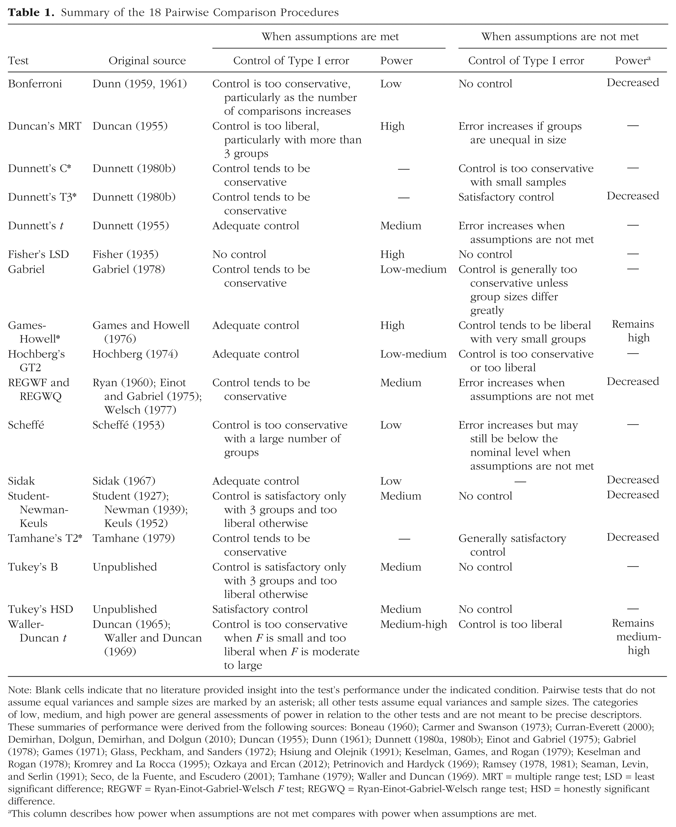
Note: Blank cells indicate that no literature provided insight into the test’s performance under the indicated condition. Pairwise tests that do not assume equal variances and sample sizes are marked by an asterisk; all other tests assume equal variances and sample sizes. The categories of low, medium, and high power are general assessments of power in relation to the other tests and are not meant to be precise descriptors. These summaries of performance were derived from the following sources: Boneau (1960); Carmer and Swanson (1973); Curran-Everett (2000); Demirhan, Dolgun, Demirhan, and Dolgun (2010); Duncan (1955); Dunn (1961); Dunnett (1980a, 1980b); Einot and Gabriel (1975); Gabriel (1978); Games (1971); Glass, Peckham, and Sanders (1972); Hsiung and Olejnik (1991); Keselman, Games, and Rogan (1979); Keselman and Rogan (1978); Kromrey and La Rocca (1995); Ozkaya and Ercan (2012); Petrinovich and Hardyck (1969); Ramsey (1978, 1981); Seaman, Levin, and Serlin (1991); Seco, de la Fuente, and Escudero (2001); Tamhane (1979); Waller and Duncan (1969). MRT = multiple range test; LSD = least significant difference; REGWF = Ryan-Einot-Gabriel-Welsch F test; REGWQ = Ryan-Einot-Gabriel-Welsch range test; HSD = honestly significant difference.

This column describes how power when assumptions are not met compares with power when assumptions are met.

Method

Simulation conditions

Table 2 shows the simulation conditions that we examined. There were three factors: number of groups, group sizes, and group variances. In short, there were three, five, or seven groups; either the sample sizes were equal at 60 per group or the ratio of the smallest to the largest group was 1:5; and either the group variances were all equal to 1 or the ratio of the smallest to the largest variance was 1:7. Two separate conditions were created when both group sizes and group variances were unequal: Either the largest group had the largest variance, or the smallest group had the largest variance.

Table 2.

Simulation Conditions

n_i	µ_i	σi2	Per-pair power^a	Omnibus power
Three groups
60/60/60	10.00/10.00/10.60	1/1/1	.91	.93
60/60/60	10.00/10.00/11.20	1/4/7	.91	.93
20/60/100	10.00/10.00/10.60	1/1/1	.68–.96	.95
20/60/100	10.00/10.00/11.39	1/4/7	.68–.96	.95
20/60/100	10.00/10.00/10.98	7/4/1	.68–.96	.95
Five groups
60/60/60/60/60	10.00/10.60/10.00/10.60/10.00	1/1/1/1/1	.91	.99
60/60/60/60/60	10.00/11.20/10.00/11.20/10.00	1/2.5/4/5.5/7	.91	.99
20/40/60/80/100	10.00/10.60/10.00/10.60/10.00	1/1/1/1/1	.59–.98	.99
20/40/60/80/100	10.00/11.34/10.00/11.34/10.00	1/2.5/4/5.5/7	.59–.98	.99
20/40/60/80/100	10.00/11.04/10.00/11.04/10.00	7/5.5/4/2.5/1	.59–.98	.99
Seven groups
60/60/60/60/60/60/60	10.00/10.60/10.00/10.60/10.00/10.60/10.00	1/1/1/1/1/1/1	.91	1.0
60/60/60/60/60/60/60	10.00/11.20/10.00/11.20/10.00/11.20/10.00	1/2/3/4/5/6/7	.91	1.0
20/33/47/60/73/87/100	10.00/10.60/10.00/10.60/10.00/10.60/10.00	1/1/1/1/1/1/1	.56–.98	1.0
20/33/47/60/73/87/100	10.00/11.27/10.00/11.27/10.00/11.27/10.00	1/2/3/4/5/6/7	.56–.98	1.0
20/33/47/60/73/87/100	10.00/11.13/10.00/11.13/10.00/11.13/10.00	7/6/5/4/3/2/1	.56–.98	1.0

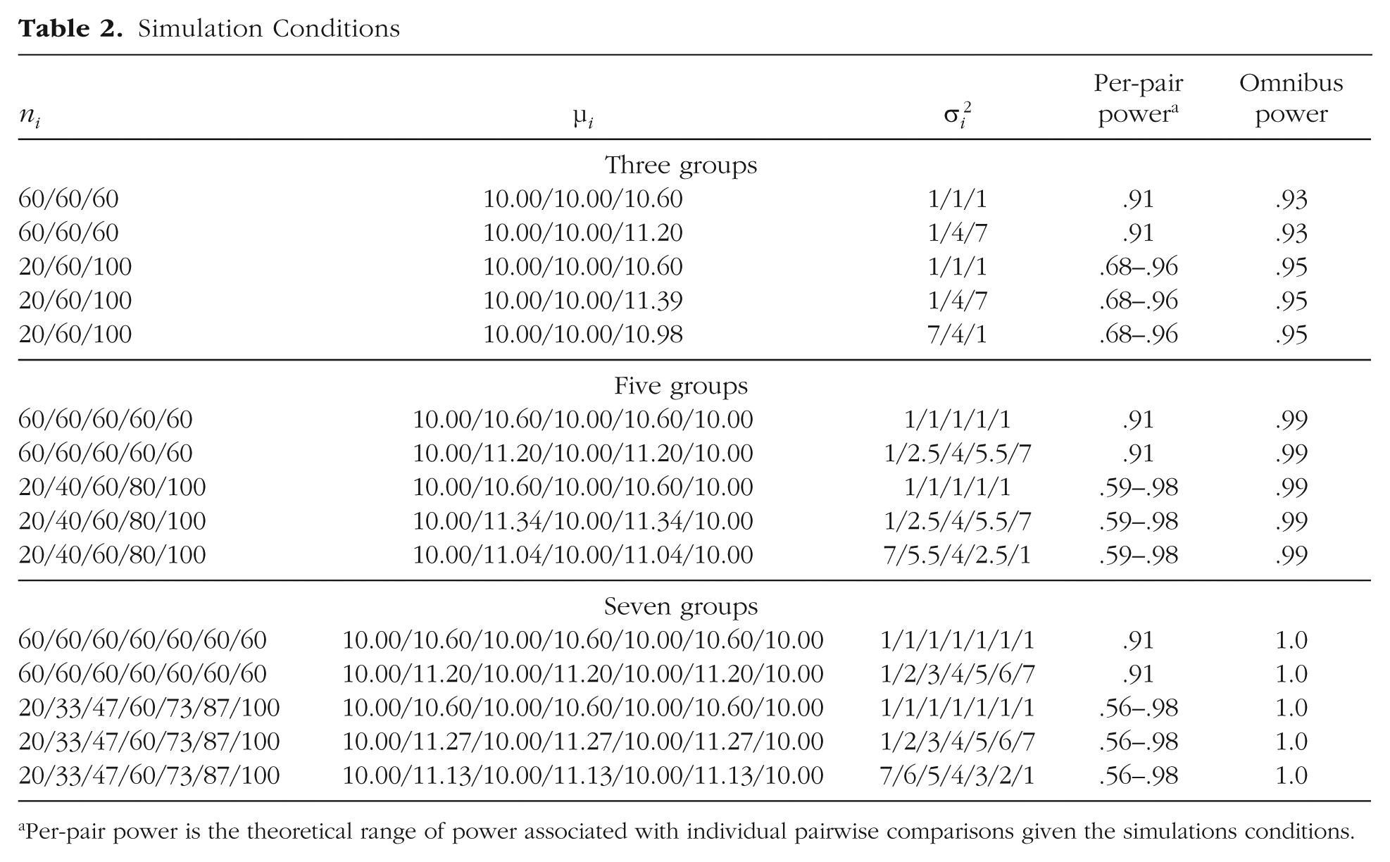
Per-pair power is the theoretical range of power associated with individual pairwise comparisons given the simulations conditions.

Thus, there were 15 data conditions in total. Number of groups, sample-size ratio, and variance ratio were crossed (3 × 2 × 2), for a total of 12 conditions. Additionally, within the cells in which both sample sizes and variances were unequal, there were two configurations of the variance ratio: In one, the largest group had the smallest variance, and in the other, the smallest group had the smallest variance; this added another 3 cells in the design. Each of these 15 data conditions was replicated 1,000 times.

Our choices for the group sizes and variances were mostly based on previous literature, but also partly based on good practice. The computing limitations at the time many of these PCPs were developed restricted the sample sizes tested to small numbers (e.g., as low as 6 in Games & Howell, 1976). Some recent evaluations of PCPs also maintained small sample sizes (as low as 4 in Demirhan et al., 2010). In part because the existing literature already discusses these small sample sizes, and in part because sampling error of group sizes so small can be detrimental to the precision of results, we chose to keep the minimum group size at 20. For the unequal-group-size conditions, the 1:5 ratio resulted in samples ranging from 20 to 100. This ratio tends to be slightly larger than what is used in the simulation literature, but is realistic for applied research, in which some groups may be much smaller than comparison groups (e.g., research comparing racial-ethnic groups). The variance ratio of 1:7 is consistent with the average in the literature, which ranges from 1:2 to 1:16.

Data

The null hypotheses in our simulations were partly true. Each group was simulated to come from a population with one of two means. Thus, some of the group means differed, and some did not. For example, in the conditions with three groups, Groups 1 and 2 had equal population means, but Group 3 had a different population mean. This allowed for both Type I errors (rejecting the null for pairs of groups with the same population mean) and computation of power (rejecting the null for pairs of groups with different population means) within each set of comparisons.

Data were simulated via SAS 9.4 using the rannor function. One set of means was fixed at 10, and the other group of means was set to a value equal to 0.6 SD above the fixed means (a medium to large effect size; J. Cohen, 1992). This is the standardized mean difference used in Cohen’s d, except that Cohen’s d is defined by the pooled within-group variances of only two groups. We instead used the square root of the mean square error term from the ANOVA as the measure of within-group variance to compute the appropriate means corresponding to 0.6 SD above the fixed means.

Given that the groups’ variances and sample sizes differed in some conditions, means also differed across conditions. The consistency across conditions comes from the difference of 0.6 SD between the group means. For the conditions in which variances differed between groups, the data were multiplied by the appropriate square root of the variance (i.e., standard deviation; see Table 2) prior to adding the appropriate mean value to maintain the 0.6-SD difference. Table 2 shows the mean assigned to each group in each condition.

The final two columns of Table 2 detail the theoretical range of maximum per-pair power and omnibus F-test power for each condition. The per-pair power values were computed as the theoretical power of independent-samples t tests comparing all simulated groups within a condition. Thus, we expected the 18 PCPs under study to provide slightly lower per-pair power than omnibus power because they were designed to control family-wise Type I error and should consequently be less powerful. The omnibus power reported in Table 2 is the theoretical power of the omnibus ANOVA F test to reject the null hypothesis that all group means are equal. We expected that any-pair power for the 18 PCPs would closely align with omnibus power.

Procedure and measures

Once the data were simulated, we wrote a macro in SPSS 24 to open the data, run the one-way ANOVA, and output the relevant PCP data to a text file. Then, the text file was read into SAS 9.4 and analyzed. The family-wise Type I error rate and all types of power (i.e., average, any-pair, and all-pairs power) were computed for each replication in each condition. Finally, the values for each of the four measures were averaged for each PCP.

Results

Type I error

The Type I error rates of the 18 PCPs in the three-group, five-group, and seven-group conditions are shown in Tables 3, 4, and 5, respectively. Largely, the tests appeared to control the Type I error rate fairly well, keeping it at least at the .05 level. In fact, most of the tests tended to be more conservative than the .05 level because only some comparisons in every condition were simulated not to have true differences. Thus, the number of comparisons that could possibly result in a Type I error was reduced to 1 out of 3 for three groups, 4 out of 10 for five groups, and 9 out of 21 for seven groups. But because these tests were designed to control Type I error in a family-wise manner, the Type I error rates we report were essentially average Type I error rates for 1, 4, and 9 comparisons when there were actually totals of 3, 10, and 21 comparisons, respectively. In other words, the tests appear to be more conservative than they really were because they controlled for more comparisons than was truly necessary. As a result, tests that had Type I error rates somewhere in the range from .01 to .05 were considered to control Type I error well.

Table 3.

Type I Error Rates for Three Groups, by Condition and Test

	Condition
Test	Equal n, equal SD	Equal n, unequal SD	Unequal n, equal SD	Unequal n, unequal SD (large^a)	Unequal n, unequal SD (small^a)
Bonferroni	.018	.002	.018	.001	.129
Duncan’s MRT	.070	.014	.088	.003	.269
Dunnett’s C*	.019	.018	.023	.014	.018
Dunnett’s T3*	.019	.016	.023	.015	.017
Dunnett’s t	—	—	—	—	—
Fisher’s LSD	.069	.015	.049	.002	.208
Gabriel	.018	.002	.021	.001	.142
Games-Howell*	.022	.018	.026	.017	.021
Hochberg’s GT2	.018	.002	.019	.001	.131
REGWF	.070	.014	.050	.002	.211
REGWQ	.070	.014	.019	.001	.137
Scheffé	.017	.002	.015	.001	.124
Sidak	.018	.002	.019	.001	.131
SNK	.070	.014	.086	.003	.264
Tamhane’s T2*	.019	.016	.023	.014	.017
Tukey’s B	.039	.006	.060	.002	.228
Tukey’s HSD	.022	.002	.020	.001	.139
Waller-Duncan t	.016	.002	.025	.001	.157

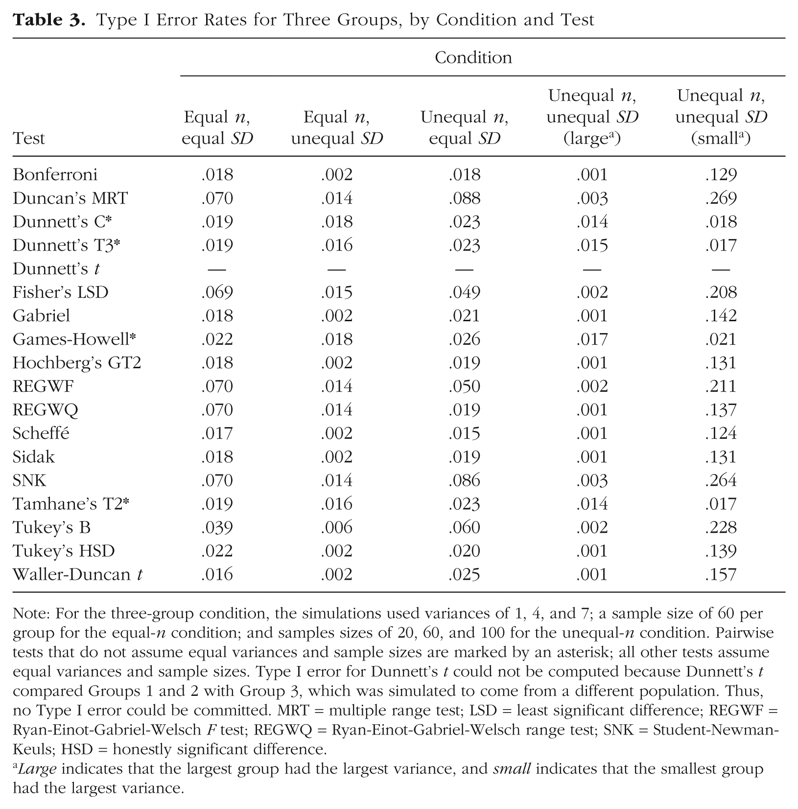
Note: For the three-group condition, the simulations used variances of 1, 4, and 7; a sample size of 60 per group for the equal-n condition; and samples sizes of 20, 60, and 100 for the unequal-n condition. Pairwise tests that do not assume equal variances and sample sizes are marked by an asterisk; all other tests assume equal variances and sample sizes. Type I error for Dunnett’s t could not be computed because Dunnett’s t compared Groups 1 and 2 with Group 3, which was simulated to come from a different population. Thus, no Type I error could be committed. MRT = multiple range test; LSD = least significant difference; REGWF = Ryan-Einot-Gabriel-Welsch F test; REGWQ = Ryan-Einot-Gabriel-Welsch range test; SNK = Student-Newman-Keuls; HSD = honestly significant difference.

Large indicates that the largest group had the largest variance, and small indicates that the smallest group had the largest variance.

Table 4.

Type I Error Rates for Five Groups, by Condition and Test

	Condition
Test	Equal n, equal SD	Equal n, unequal SD	Unequal n, equal SD	Unequal n, unequal SD (large^a)	Unequal n, unequal SD (small^a)
Bonferroni	.017	.022	.017	.003	.085
Duncan’s MRT	.138	.140	.170	.023	.327
Dunnett’s C*	.024	.024	.021	.016	.020
Dunnett’s T3*	.021	.017	.018	.015	.016
Dunnett’s t	.025	.039	.031	.012	.082
Fisher’s LSD	.169	.162	.186	.069	.327
Gabriel	.017	.022	.023	.003	.102
Games-Howell*	.025	.025	.022	.017	.020
Hochberg’s GT2	.017	.022	.018	.003	.088
REGWF	.047	.056	.069	.013	.167
REGWQ	.045	.055	.018	.003	.078
Scheffé	.008	.011	.010	.001	.050
Sidak	.017	.022	.018	.003	.088
SNK	.093	.101	.104	.016	.251
Tamhane’s T2*	.020	.017	.018	.015	.016
Tukey’s B	.044	.054	.050	.001	.193
Tukey’s HSD	.019	.024	.022	.006	.093
Waller-Duncan t	.041	.044	.052	.001	.201

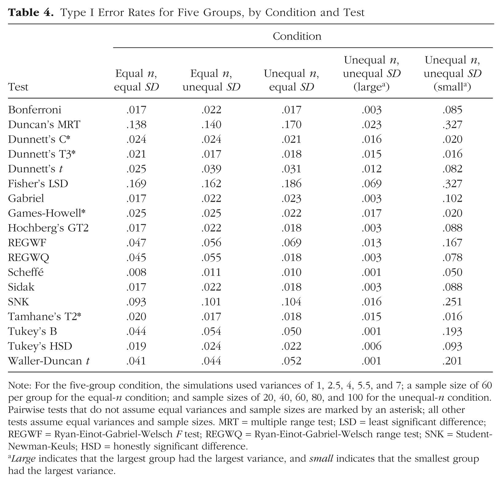
Note: For the five-group condition, the simulations used variances of 1, 2.5, 4, 5.5, and 7; a sample size of 60 per group for the equal-n condition; and sample sizes of 20, 40, 60, 80, and 100 for the unequal-n condition. Pairwise tests that do not assume equal variances and sample sizes are marked by an asterisk; all other tests assume equal variances and sample sizes. MRT = multiple range test; LSD = least significant difference; REGWF = Ryan-Einot-Gabriel-Welsch F test; REGWQ = Ryan-Einot-Gabriel-Welsch range test; SNK = Student-Newman-Keuls; HSD = honestly significant difference.

Large indicates that the largest group had the largest variance, and small indicates that the smallest group had the largest variance.

Table 5.

Type I Error Rates for Seven Groups, by Condition and Test

	Condition
Test	Equal n, equal SD	Equal n, unequal SD	Unequal n, equal SD	Unequal n, unequal SD (large^a)	Unequal n, unequal SD (small^a)
Bonferroni	.018	.034	.016	.010	.094
Duncan’s MRT	.237	.230	.242	.054	.456
Dunnett’s C*	.028	.020	.023	.030	.023
Dunnett’s T3*	.023	.018	.021	.027	.021
Dunnett’s t	.022	.067	.029	.023	.080
Fisher’s LSD	.313	.288	.295	.174	.480
Gabriel	.019	.034	.020	.010	.110
Games-Howell*	.031	.021	.028	.035	.026
Hochberg’s GT2	.019	.034	.016	.010	.094
REGWF	.053	.058	.059	.025	.178
REGWQ	.055	.066	.024	.015	.104
Scheffé	.003	.005	.003	.003	.038
Sidak	.019	.024	.016	.010	.094
SNK	.096	.111	.118	.014	.282
Tamhane’s T2*	.023	.018	.021	.027	.019
Tukey’s B	.058	.067	.088	.002	.229
Tukey’s HSD	.025	.036	.021	.011	.110
Waller-Duncan t	.081	.097	.122	.010	.280

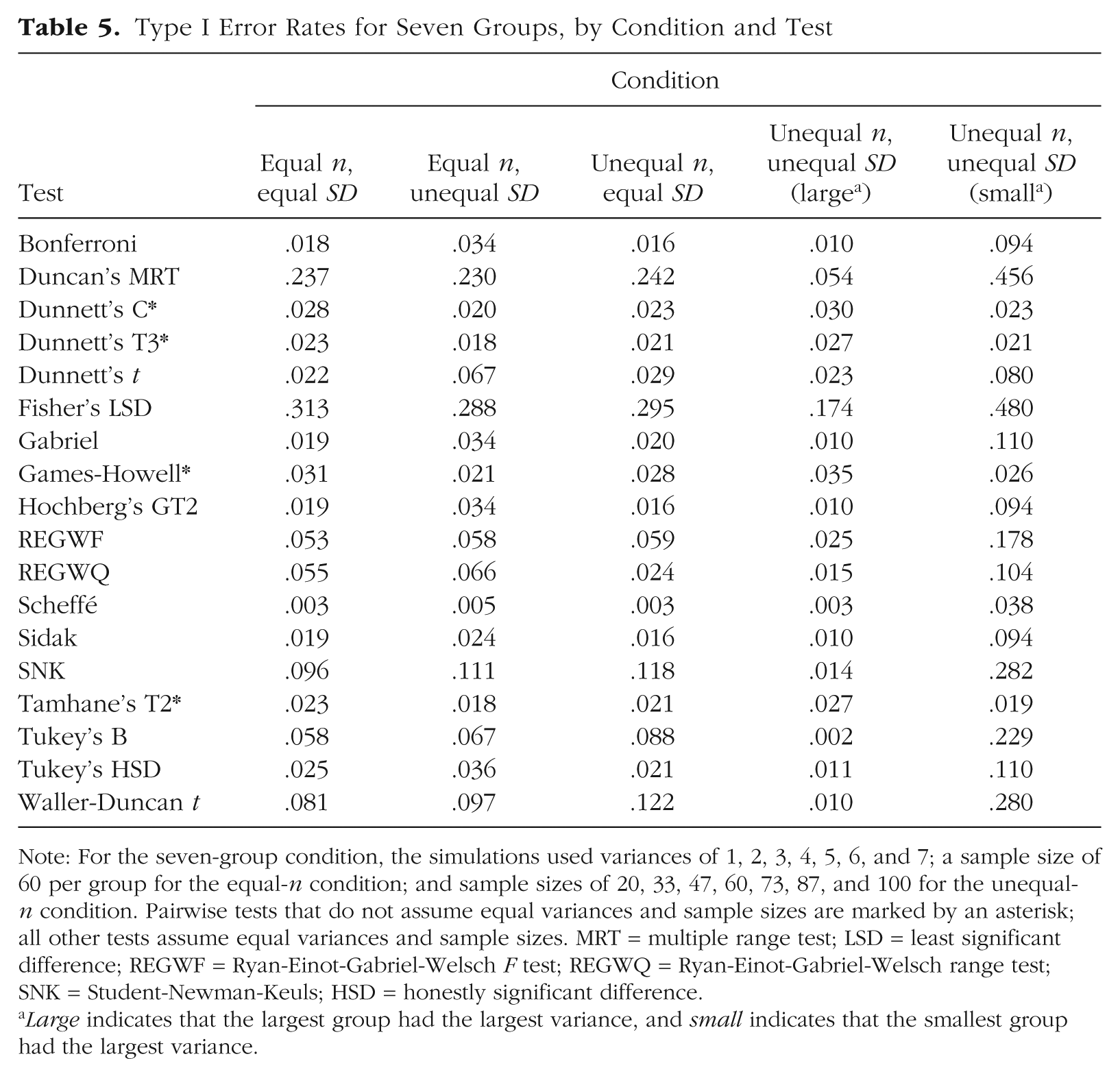
Note: For the seven-group condition, the simulations used variances of 1, 2, 3, 4, 5, 6, and 7; a sample size of 60 per group for the equal-n condition; and sample sizes of 20, 33, 47, 60, 73, 87, and 100 for the unequal-n condition. Pairwise tests that do not assume equal variances and sample sizes are marked by an asterisk; all other tests assume equal variances and sample sizes. MRT = multiple range test; LSD = least significant difference; REGWF = Ryan-Einot-Gabriel-Welsch F test; REGWQ = Ryan-Einot-Gabriel-Welsch range test; SNK = Student-Newman-Keuls; HSD = honestly significant difference.

Large indicates that the largest group had the largest variance, and small indicates that the smallest group had the largest variance.

Results when assumptions were met

In the equal-n, equal-SD condition, Duncan’s MRT, Fisher’s LSD test, and the SNK test were all too liberal for all group sizes. When there were three groups, the REGWQ and REGWF tests were also too liberal, but all the other tests controlled Type I error adequately. With five groups, every test but Duncan’s MRT, Fisher’s LSD test, and the SNK test controlled Type I error adequately. However, with seven groups, the Waller-Duncan t test also became too liberal. Some of the tests (REGWF, REGWQ, and Tukey’s B) controlled Type I error near the .05 level, whereas other tests were conservative (e.g., the Scheffé test).

Results when assumptions were not met

Equal n, unequal SD

With three groups, all the tests controlled Type I error below the .05 level. Many were quite conservative in their control (error rates < .01), but the values were less extreme (> .01) for Duncan’s MRT and the Dunnett’s C, Dunnett’s T3, Games-Howell, Fisher’s LSD, REGWF, REGWQ, SNK, and Tamhane’s T2 tests. The tests became more liberal with five groups, and Duncan’s MRT, Fisher’s LSD test, and the SNK test no longer controlled Type I error near the .05 level. The REGWF, REGWQ, Tukey’s B, and Waller-Duncan t tests all controlled Type I error near the .05 level (in three cases, slightly above .05). Results for five groups and seven groups were largely similar, except that Dunnett’s t test and the Waller-Duncan t test also became slightly too liberal for seven groups.

Unequal n, equal SD

In this condition, Duncan’s MRT and the SNK test did not control Type I error well with three groups. Further, Fisher’s LSD test, the REGWF test, and Tukey’s B test had error rates near or slightly above .05. All the other tests performed well with three groups. With five groups, Duncan’s MRT, Fisher’s LSD test, the REGWF test, and the SNK test did not control Type I error well. All the other tests maintained Type I error rates below or near .05 (.05 for Tukey’s B test and .052 for the Waller-Duncan test). With seven groups, Duncan’s MRT, Fisher’s LSD test, the SNK test, Tukey’s B test, and the Waller-Duncan t test did not control Type I error well. The REGWF test performed adequately, but with slightly inflated Type I error rates. All the other tests controlled Type I error adequately, and the Scheffé test was the most conservative (possibly too conservative).

Unequal n, unequal SD (largest group had the largest variance)

In this condition, all the tests except those designed for unequal group variances and sample sizes (i.e., Dunnett’s C, Dunnett’s T3, Games-Howell, and Tamhane’s T2) were quite conservative for three groups (error rates < .01). For five groups, half the tests were still conservative, though Duncan’s MRT, Dunnett’s t test, the REGWF test, and the SNK test had more typical Type I error rates, as did the Dunnett’s C, Dunnett’s T3, Games-Howell, and Tamhane’s T2 tests. Additionally, Fisher’s LSD test was too liberal with five groups. With seven groups, Fisher’s LSD test did not control Type I error. Otherwise, the tests performed adequately with the exception of the Scheffé and Tukey’s B tests, which were still conservative.

Unequal n, unequal SD (smallest group had the largest variance)

Only Dunnett’s C test, Dunnett’s T3 test, the Games-Howell test, and Tamhane’s T2 test controlled Type I error adequately for all group sizes. The Scheffé test had adequate Type I error rates in the five- and seven-group conditions, though this was likely due to its inherent conservative tendencies. Some tests exceeded the nominal Type I error rate by about .05 for some group sizes, but other tests had Type I error rates nearly 10 times the nominal rate in the seven-group condition.

Power

A test can have high power because it does not control Type I error. Essentially, a test could lead researchers to reject virtually every null hypothesis, and thus result in high Type I error rates, but simultaneously detect every statistically significant difference, and thus have high power. Because researchers can never know if significant results are Type I errors or not, blindly using a test that provides high power at the expense of increased Type I error rates is poor practice. Thus, although we report power for all 18 of the PCPs in the appendix (Tables A1 –A3), in this section we focus on power for the tests that maintained control over Type I error in all conditions: Dunnett’s C test, Dunnett’s T3 test, the Games-Howell test, and Tamhane’s T2 test.

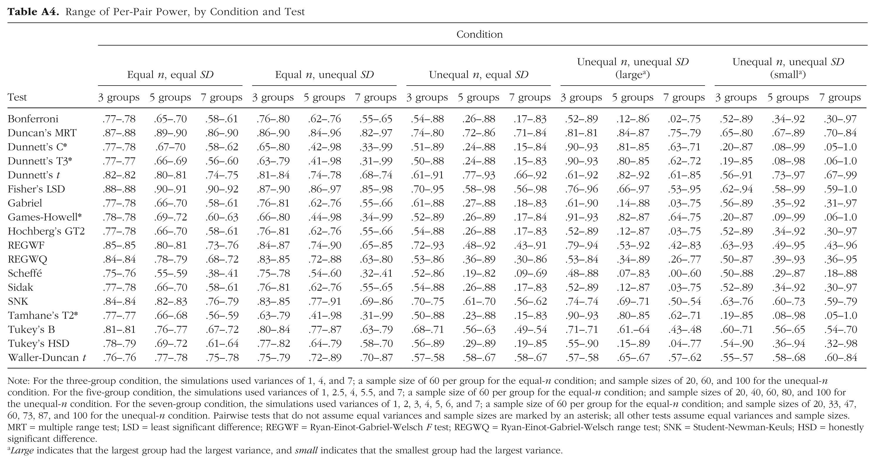
We computed a test’s any-pair power as the proportion of replications that correctly identified at least one statistically significant difference. All-pairs power was computed as the proportion of replications in which every statistically significant difference was correctly identified. Average power was computed as the proportion of simulated pairwise differences detected averaged over the 1,000 replications. Additionally, Table A4 in the appendix shows the range of per-pair power for each PCP in each condition. Power levels for Dunnett’s C test, Dunnett’s T3 test, the Games-Howell test, and Tamhane’s T2 test are shown in Figures 1, 2, and 3 for three, five, and seven groups, respectively.

Fig. 1.

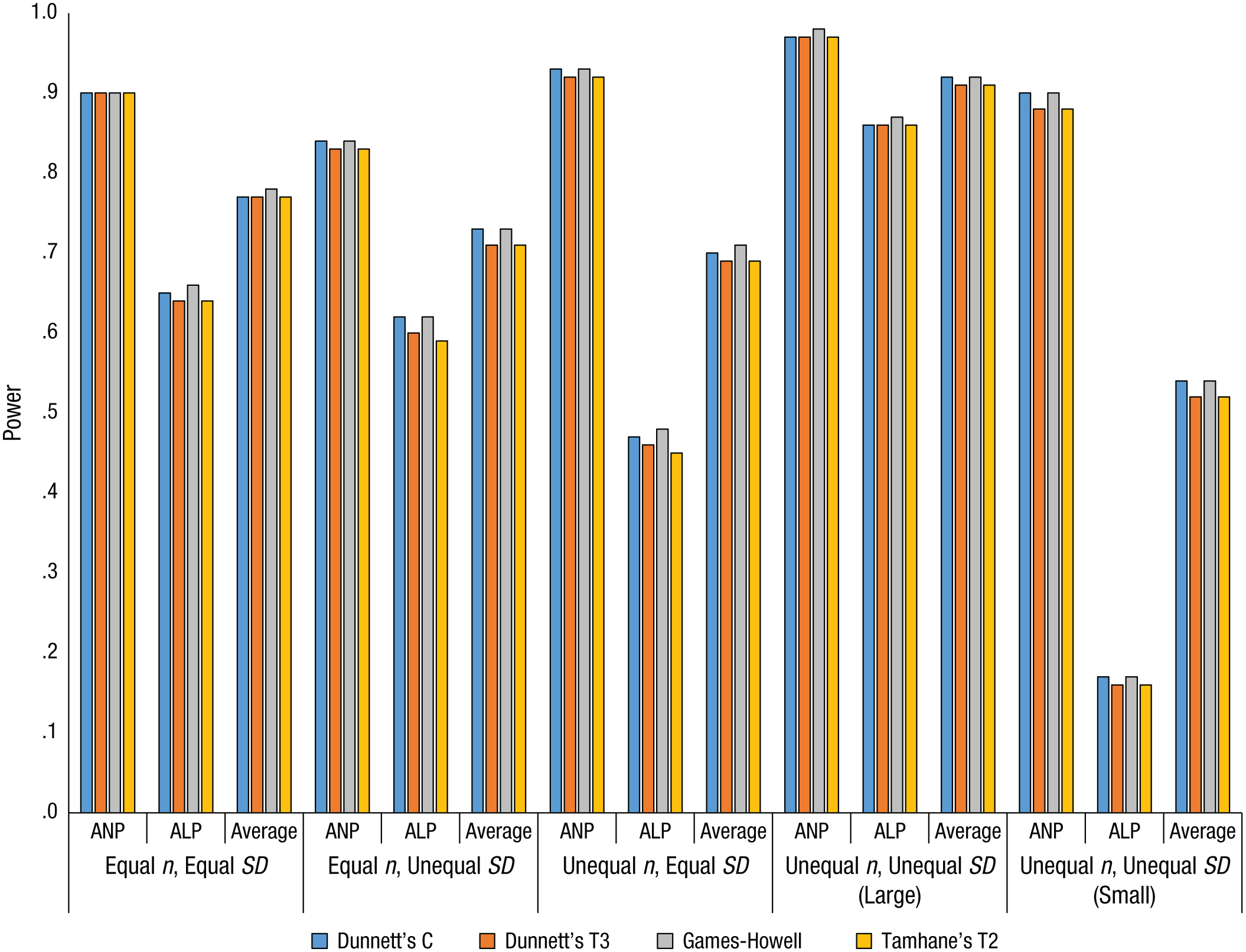
Power values for Dunnett’s C test, Dunnett’s T3 test, the Games-Howell test, and Tamhane’s T2 test with three groups. Large indicates that the largest group had the largest variance, and small indicates that the smallest group had the largest variance. ANP = any-pair power; ALP = all-pairs power; Average = average power.

Fig. 2.

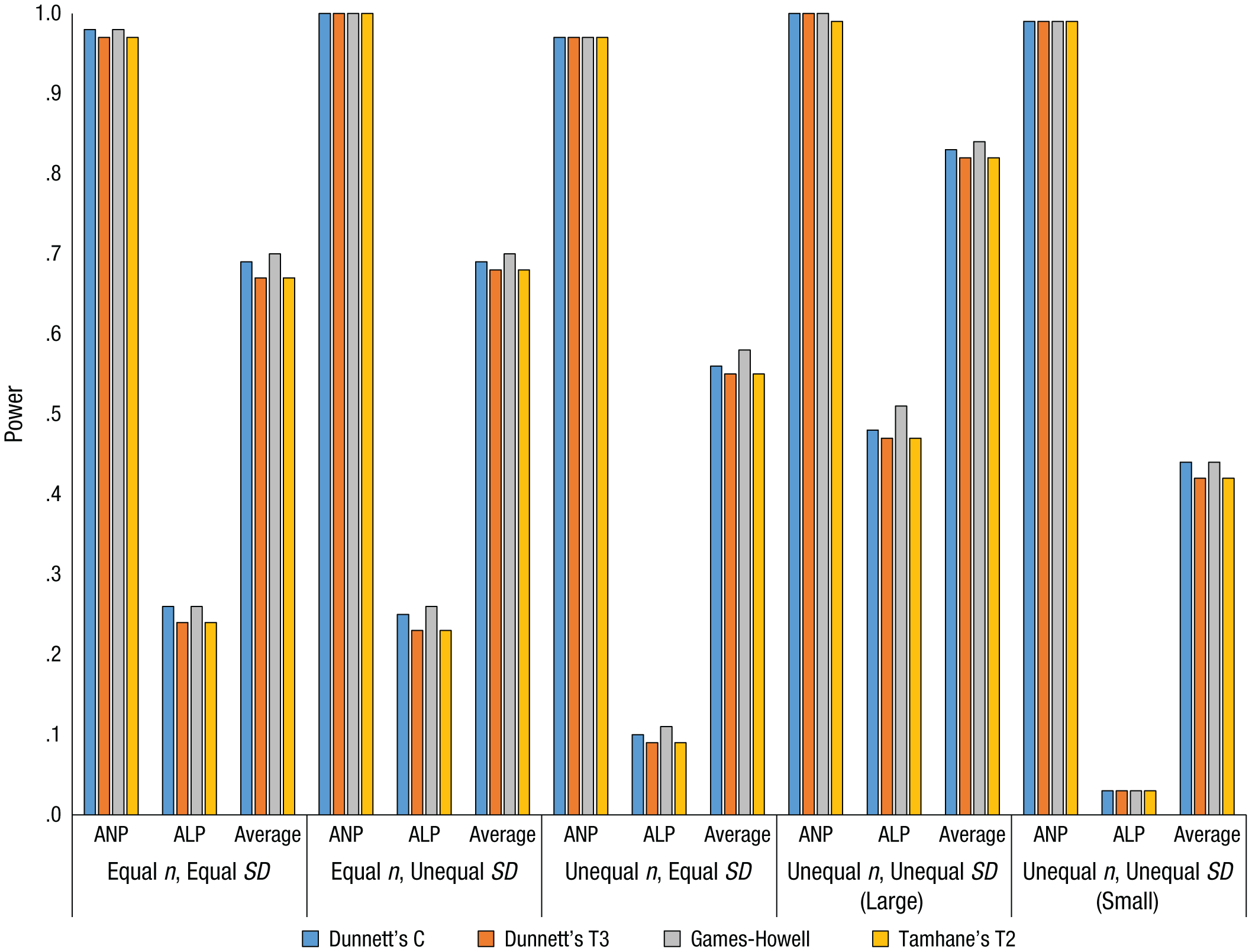
Power values for Dunnett’s C test, Dunnett’s T3 test, the Games-Howell test, and Tamhane’s T2 test with five groups. Large indicates that the largest group had the largest variance, and small indicates that the smallest group had the largest variance. ANP = any-pair power; ALP = all-pairs power; Average = average power.

Fig. 3.

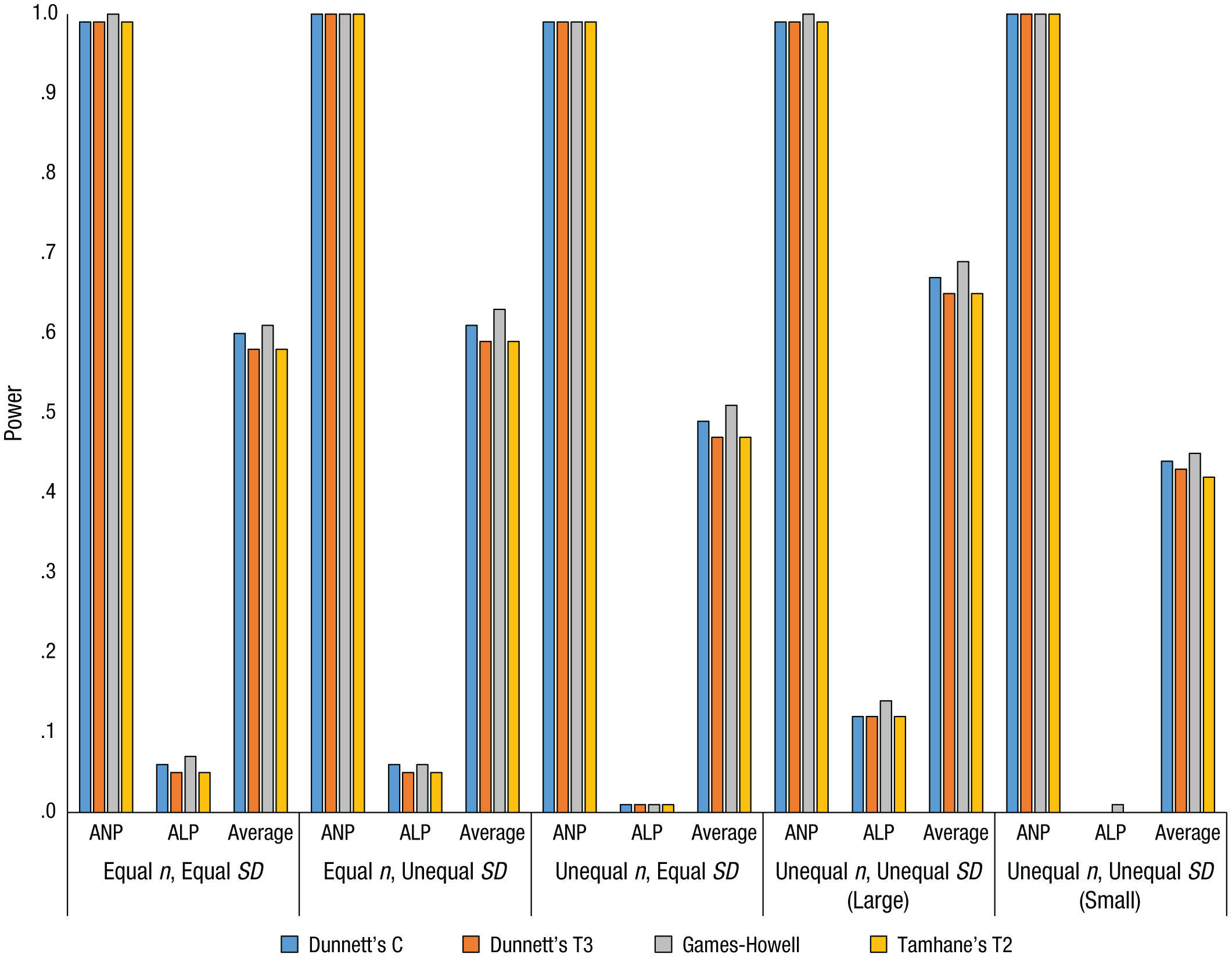
Power values for Dunnett’s C test, Dunnett’s T3 test, the Games-Howell test, and Tamhane’s T2 test with seven groups. Large indicates that the largest group had the largest variance, and small indicates that the smallest group had the largest variance. ANP = any-pair power; ALP = all-pairs power; Average = average power.

Results when assumptions were met

In the equal-n, equal-SD condition, all four of these tests provided high any-pair power that increased as the number of groups increased (Tables A1 –A3). Intuitively, this makes sense, because as the number of groups increased, so did the number of comparisons. Consequently, it was more likely that at least one of the comparisons would accurately reject the null hypothesis. Similar logic, but in reverse, explains the decrease in all-pairs power from around .65 for three groups to around .05 for seven groups: The more comparisons are possible, the less likely it is to correctly reject all of the null hypotheses that should be rejected. Average power decreased as the number of groups increased, changing from just under .80 for three groups to around .60 for seven groups. Per-pair power decreased slightly as the number of groups increased (Table A4).

Results when assumptions were not met

Equal n, unequal SD

For Dunnett’s C test, Dunnett’s T3 test, the Games-Howell test, and Tamhane’s T2 test, all-pairs power in the equal-n, unequal-SD condition was nearly identical to that in the equal-n, equal-SD condition (Tables A1 –A3). Any-pair power was just under .85 for three groups, but maxed out around 1.0 (i.e., 100% of replications) for five and seven groups. Average power decreased as the number of groups did, as in the equal-n, equal-SD condition. In addition, the gap between the lowest per-pair power and the highest per-pair power increased with the number of groups (i.e., the variability of per-pair power increased) to a much larger extent than in the equal-n, equal-SD condition (Table A4).

Unequal n, equal SD

Any-pair power for these four tests was high (> .90) regardless of the number of groups (Tables A1 –A3). In contrast, all-pairs power was moderately high (close to .50) for three groups and decreased substantially as the number of groups increased to five (power around .10) and to seven (power near 0). Average power showed a similar though less extreme trend, decreasing as the number of groups increased. This decrease was more pronounced for the change from three groups to five groups than for the change from five groups to seven groups. Further, there was again variation in the per-pair power, and the range widened as the number of groups increased (Table A4).

Unequal n, unequal SD (largest group had the largest variance)

All measures of power for Dunnett’s C test, Dunnett’s T3 test, the Games-Howell test, and Tamhane’s T2 test were at their highest or near 1.0 in this condition (Tables A1 –A3), which seems counterintuitive at first. However, recall that these tests were designed for unequal variances and sample sizes. Power tended to be lower for most of the other tests in this condition (Tables A1 –A3). In any event, any-pair power for Dunnett’s C test, Dunnett’s T3 test, the Games-Howell test, and Tamhane’s T2 test was close to 1 in this condition regardless of group size. All-pairs power followed the other conditions in decreasing as the number of groups increased, because of the increased number of tests. However, all-pairs power was around .50 with five groups, and with seven groups, all-pairs power was still higher than in the other conditions, though low at around .10. Average power was higher than in the equal-n, equal-SD condition, and per-pair power had little variation (Table A4).

Unequal n, unequal SD (smallest group had the largest variance)

Although any-pair power for Dunnett’s C test, Dunnett’s T3 test, the Games-Howell test, and Tamhane’s T2 test was comparable in this condition and the other conditions, all-pairs power for these four tests was at its lowest in this condition, at or approaching 0 with seven groups (Tables A1 –A3). Average power was also at its minimum, slightly above .50 for three groups and dipping to near .40 for seven groups. This drop appears to be due to the interaction of sample size and group variance. Specifically, when there were seven groups in this condition, the comparison of the two smallest groups (1 and 2) had the lowest per-pair power. However, when there were seven groups in the unequal-n, unequal-SD condition with the largest variance associated with the largest group, the lowest per-pair power was found when the largest groups were compared (i.e., groups 6 and 7). In other words, power was lowest for the pairs with the greatest within-group variance. Power was particularly low when the smallest groups had the largest variance because both sample size and variance contribute to the standard error of the difference between groups.

Summary

Duncan’s MRT, Fisher’s LSD test, the SNK test, and the Waller-Duncan t test did not control Type I error in a large number of conditions. Other tests maintained Type I error in most conditions, but were too conservative in the unequal-n, unequal-SD condition when the largest group had the largest variance and were too liberal in the unequal-n, unequal-SD condition when the smallest group had the largest variance. Only Dunnett’s C test, Dunnett’s T3 test, the Games-Howell test, and Tamhane’s T2 test adequately controlled Type I error in all conditions. Any-pair power of the four tests that maintained control over Type I error in all conditions was high in all conditions, but all-pairs power decreased as the number of groups increased in all conditions. For these four tests, the highest power levels were found in the unequal-n, unequal-SD condition in which the largest group had the largest variance, and the lowest power levels were found in the unequal-n, unequal-SD condition in which the smallest group had the largest variance. Average power remained fairly consistent across conditions compared with per-pair power, which varied greatly.

Discussion

Type I error

Our results for Type I error are both disappointing and encouraging. First, the vast majority of tests (Bonferroni, Duncan’s MRT, Dunnett’s t, Gabriel, Hochberg’s GT2, Fisher’s LSD, REGWF, REGWQ, Scheffé, Sidak, SNK, Tukey’s B, Tukey’s HSD, and Waller-Duncan t) did not consistently control Type I error near the nominal level when assumptions were violated. In general, increasing the number of groups in the model resulted in worse Type I error rates—in some cases, rates that were too conservative (e.g., Scheffé), and in other cases, rates that were too liberal (e.g., Fisher’s LSD, Duncan’s MRT). Inflated Type I error rates were as high as 48.0% in the simulation conditions.

Fortunately, the four tests designed for use under violations of assumptions—Dunnett’s T3 test, Dunnett’s C test, the Games-Howell test, and Tamhane’s T2 test—controlled Type I error adequately in all conditions. Thus, the adjustment to the degrees of freedom coupled with a weighted pooled-variance term based on only the two groups being compared was able to account for the heterogeneity and unequal group sizes simulated in this study. We adopt a “better safe than sorry” mentality for PCPs and suggest that introductory and intermediate statistics professors recommend one of these four tests to their students. Although certain common tests also controlled Type I error adequately when assumptions were met (e.g., Tukey’s HSD), this data condition is unrealistic in real-data research (i.e., groups are often unequal, and population variances are almost never equal for demographically based groups). We did not examine the performance of tests such as Tukey’s HSD under the minor violations of assumptions that are more likely in real-data research, but the “better safe than sorry” mentality suggests that a test that will control the Type I error rate under even the more extreme violations we used in our simulations is the most logical choice, as long as power is not negatively affected.

If power is not a consideration and controlling Type I error is the only concern, using a more conservative test, such as the Bonferroni or Scheffé test, may be attractive. However, even these tests had inflated Type I error rates in the unequal-n, unequal-SD condition when the smallest group had the largest variance. Further, in real-data research, it is impossible to know if a Type I error is being committed and what the empirical Type I error rate is. Thus, although researchers can be reasonably sure that the Scheffé test maintains the nominal .05 family-wise Type I error rate in most situations, they cannot be positive. Instead, they should use a test that has been shown to maintain the nominal Type I error rate in all studied conditions, such as one of the four tests designed for assumption violations. This argument can be extended to situations in which statistical power is a consideration, and we do so in the next section.

Power

The control of Type I error provided by Dunnett’s T3 test, Dunnett’s C test, the Games-Howell test, and Tamhane’s T2 test is not as beneficial as it might seem if it comes at the cost of lower power compared with alternative tests. Therefore, it is useful to compare the power of these four tests with the power of the others, excluding those tests that did not control Type I error in the majority of conditions (Duncan’s MRT, Fisher’s LSD test, and the SNK test) and excluding Dunnett’s t test (because it compares all groups with one control group rather than conducting all pairwise comparisons). This comparison reveals that the average power for these four tests is roughly the same as the power of any other test within a given condition in almost all cases (see the appendix). The price for the tight Type I error control provided by Dunnett’s T3 test, Dunnett’s C test, the Games-Howell test, and Tamhane’s T2 test is practically insignificantly lower power rates. The REGWF and REGWQ tests did provide meaningfully higher all-pairs and average power in several conditions while simultaneously controlling Type I error rates, but these tests’ lack of Type I error control in several other conditions does not make them attractive options.

An argument could be made for purposefully choosing a PCP that provides high power at the expense of Type I error control in exploratory research, when there is no well-established theory to help dictate comparisons of interest. Exploratory researchers may be more concerned with detecting any statistically significant differences than with controlling Type I error, so that their results can inform later follow-up studies. Essentially, exploratory studies are theory-generating studies instead of theory-confirming studies. PCPs are in some ways exploratory by nature because they examine all pairwise comparisons with no a priori hypotheses. However, we argue that instead of switching to a PCP with known higher power but unknown Type I error control, it is better to use one of the tests designed for assumption violations (i.e., Dunnett’s C, Dunnett’s T3, Games-Howell, or Tamhane’s T2) and simply increase the nominal Type I error rate from .05 to something like .10 or .15. With this approach, the experimental Type I error rate is still known, but at the same time power is increased to account for the exploratory nature of the research.

Limitations

As is the case with any simulation study, an obvious limitation of this study is the restricted set of conditions. Real-data research does not conform to the conditions we tested; rather, the conditions tested were intended to be generally similar to, if not more extreme than, real-data situations. That is, the simulation conditions were designed to reflect reasonable to major deviations in group size and variances between groups, with the thought that at least some real-data group sizes and variances would fall in the same “ballpark” as the simulation or that the tests would perform better in less extreme situations.

Also, our data were simulated from a normal population, whereas real data are rarely perfectly normally distributed. We chose not to simulate nonnormal data in part to reduce the scope of this study, but primarily because OLS estimation tends to be fairly robust to nonnormality. A third limitation is that we did not examine the effects of dependencies within the data, such as what may be found with cluster sampling that results in nested data. Some research has shown that even mild levels of dependence can seriously inflate Type I error rates (Demirhan et al., 2010; Seco, de la Fuente, & Escudero, 2001). ANOVA provides a framework for modeling a cluster effect to combat the nuisance of inflated Type I error rates: The effect is simply modeled as a random factor. For example, if students are nested within classes, one can model the class effect by entering a section-number variable as a separate grouping factor. In any event, our recommendation to use the tests designed for assumption violations should be considered only when data are close to normally distributed and independent.

Conclusions and recommendation

When the assumptions of equal sample sizes and variances were violated, only four tests adequately maintained the Type I error rate: Dunnett’s C, Dunnett’s T3, Games-Howell, and Tamhane’s T2. All four tests provided similar levels of any-pair, all-pairs, and average power, though the Games-Howell provided a slight edge. Thus, for strict control of Type I error and acceptable power, we recommend utilizing the Games-Howell test, Dunnett’s C test, Dunnett’s T3 test, or Tamhane’s T2 procedure with normal and independent data (we note that our recommendations are similar to those of Keselman & Rogan, 1977) and teaching any of these methods in introductory and intermediate statistics courses. Further research is required for recommendations for nonnormal and dependent data.

Although other tests may be attractive because of their higher power, we do not recommend their use because they did not control Type I error at the nominal level in several conditions. We suggest that instead of choosing a test that provides high power at the expense of unknown empirical Type I error, students should use the Games-Howell procedure (or one of the other three tests designed for assumption violations) with an increased nominal alpha level to achieve higher power levels with a known Type I error rate. Increasing alpha provides greater power at the expense of more Type I errors, but the Type I error rate will be controlled at the value of the nominal alpha, which is not the case for tests that do not control Type I error. Using one of the four procedures designed for assumption violations with a less strict alpha level may be particularly useful for exploratory research, in which controlling Type I error at the typical .05 level may be of less importance than detecting significant differences to generate follow-up hypotheses.

Supplemental Material

DS_10.1177_2515245918808784 – Supplemental material for An Updated Recommendation for Multiple Comparisons

Supplemental material, DS_10.1177_2515245918808784 for An Updated Recommendation for Multiple Comparisons by Derek C. Sauder and Christine E. DeMars in Advances in Methods and Practices in Psychological Science

Footnotes

Appendix

Table A4.

Range of Per-Pair Power, by Condition and Test

	Condition
	Equal n, equal SD			Equal n, unequal SD			Unequal n, equal SD			Unequal n, unequal SD (large^a)			Unequal n, unequal SD (small^a)
Test	3 groups	5 groups	7 groups	3 groups	5 groups	7 groups	3 groups	5 groups	7 groups	3 groups	5 groups	7 groups	3 groups	5 groups	7 groups
Bonferroni	.77–.78	.65–.70	.58–.61	.76–.80	.62–.76	.55–.65	.54–.88	.26–.88	.17–.83	.52–.89	.12–.86	.02–.75	.52–.89	.34–.92	.30–.97
Duncan’s MRT	.87–.88	.89–.90	.86–.90	.86–.90	.84–.96	.82–.97	.74–.80	.72–.86	.71–.84	.81–.81	.84–.87	.75–.79	.65–.80	.67–.89	.70–.84
Dunnett’s C*	.77–.78	.67–70	.58–.62	.65–.80	.42–.98	.33–.99	.51–.89	.24–.88	.15–.84	.90–.93	.81–.85	.63–.71	.20–.87	.08–.99	.05–1.0
Dunnett’s T3*	.77–.77	.66–.69	.56–.60	.63–.79	.41–.98	.31–.99	.50–.88	.24–.88	.15–.83	.90–.93	.80–.85	.62–.72	.19–.85	.08–.98	.06–1.0
Dunnett’s t	.82–.82	.80–.81	.74–.75	.81–.84	.74–.78	.68–.74	.61–.91	.77–.93	.66–.92	.61–.92	.82–.92	.61–.85	.56–.91	.73–.97	.67–.99
Fisher’s LSD	.88–.88	.90–.91	.90–.92	.87–.90	.86–.97	.85–.98	.70–.95	.58–.98	.56–.98	.76–.96	.66–.97	.53–.95	.62–.94	.58–.99	.59–1.0
Gabriel	.77–.78	.66–.70	.58–.61	.76–.81	.62–.76	.55–.66	.61–.88	.27–.88	.18–.83	.61–.90	.14–.88	.03–.75	.56–.89	.35–.92	.31–.97
Games-Howell*	.78–.78	.69–.72	.60–.63	.66–.80	.44–.98	.34–.99	.52–.89	.26–.89	.17–.84	.91–.93	.82–.87	.64–.75	.20–.87	.09–.99	.06–1.0
Hochberg’s GT2	.77–.78	.66–.70	.58–.61	.76–.81	.62–.76	.55–.66	.54–.88	.26–.88	.17–.83	.52–.89	.12–.87	.03–.75	.52–.89	.34–.92	.30–.97
REGWF	.85–.85	.80–.81	.73–.76	.84–.87	.74–.90	.65–.85	.72–.93	.48–.92	.43–.91	.79–.94	.53–.92	.42–.83	.63–.93	.49–.95	.43–.96
REGWQ	.84–.84	.78–.79	.68–.72	.83–.85	.72–.88	.63–.80	.53–.86	.36–.89	.30–.86	.53–.84	.34–.89	.26–.77	.50–.87	.39–.93	.36–.95
Scheffé	.75–.76	.55–.59	.38–.41	.75–.78	.54–.60	.32–.41	.52–.86	.19–.82	.09–.69	.48–.88	.07–.83	.00–.60	.50–.88	.29–.87	.18–.88
Sidak	.77–.78	.66–.70	.58–.61	.76–.81	.62–.76	.55–.65	.54–.88	.26–.88	.17–.83	.52–.89	.12–.87	.03–.75	.52–.89	.34–.92	.30–.97
SNK	.84–.84	.82–.83	.76–.79	.83–.85	.77–.91	.69–.86	.70–.75	.61–.70	.56–.62	.74–.74	.69–.71	.50–.54	.63–.76	.60–.73	.59–.79
Tamhane’s T2*	.77–.77	.66–.68	.56–.59	.63–.79	.41–.98	.31–.99	.50–.88	.23–.88	.15–.83	.90–.93	.80–.85	.62–.71	.19–.85	.08–.98	.05–1.0
Tukey’s B	.81–.81	.76–.77	.67–.72	.80–.84	.77–.87	.63–.79	.68–.71	.56–.63	.49–.54	.71–.71	.61.–64	.43–.48	.60–.71	.56–.65	.54–.70
Tukey’s HSD	.78–.79	.69–.72	.61–.64	.77–.82	.64–.79	.58–.70	.56–.89	.29–.89	.19–.85	.55–.90	.15–.89	.04–.77	.54–.90	.36–.94	.32–.98
Waller-Duncan t	.76–.76	.77–.78	.75–.78	.75–.79	.72–.89	.70–.87	.57–.58	.58–.67	.58–.67	.57–.58	.65–.67	.57–.62	.55–.57	.58–.68	.60–.84

Note: For the three-group condition, the simulations used variances of 1, 4, and 7; a sample size of 60 per group for the equal-n condition; and sample sizes of 20, 60, and 100 for the unequal-n condition. For the five-group condition, the simulations used variances of 1, 2.5, 4, 5.5, and 7; a sample size of 60 per group for the equal-n condition; and sample sizes of 20, 40, 60, 80, and 100 for the unequal-n condition. For the seven-group condition, the simulations used variances of 1, 2, 3, 4, 5, 6, and 7; a sample size of 60 per group for the equal-n condition; and sample sizes of 20, 33, 47, 60, 73, 87, and 100 for the unequal-n condition. Pairwise tests that do not assume equal variances and sample sizes are marked by an asterisk; all other tests assume equal variances and sample sizes. MRT = multiple range test; LSD = least significant difference; REGWF = Ryan-Einot-Gabriel-Welsch F test; REGWQ = Ryan-Einot-Gabriel-Welsch range test; SNK = Student-Newman-Keuls; HSD = honestly significant difference.

Large indicates that the largest group had the largest variance, and small indicates that the smallest group had the largest variance.

Action Editor

Alexa Tullett served as action editor for this article.

Author Contributions

D. C. Sauder generated the idea for the study. D. C. Sauder and C. E. DeMars jointly programmed, ran, and analyzed the data from the simulations. D. C. Sauder wrote the manuscript, and C. E. DeMars provided substantial revisions. Both authors approved the final submitted version of the manuscript.

ORCID iD

Christine E. DeMars

Declaration of Conflicting Interests

The author(s) declared that there were no conflicts of interest with respect to the authorship or the publication of this article.

References

Aiken

L. S.

West

S. G.

Millsap

R. E.

(2008). Doctoral training in statistics, measurement, and methodology in psychology: Replication and extension of Aiken, West, Sechrest, and Reno’s (1990) survey of PhD programs in North America. American Psychologist, 63, 32–50.

Andreassen

C. S.

Pallesen

Griffiths

M. D.

(2017). The relationship between addictive use of social media, narcissism, and self-esteem: Findings from a large national survey. Addictive Behaviors, 64, 287–293.

Bohrnstedt

G. W.

Carter

T. M.

(1971). Robustness in re-gression analysis. Sociological Methodology, 3, 118–146.

Boneau

C. A.

(1960). The effects of violations of assumptions underlying the t test. Psychological Bulletin, 57, 49–64.

Carmer

S. G.

Swanson

M. R.

(1973). An evaluation of ten pairwise multiple comparison procedures by Monte Carlo methods. Journal of the American Statistical Association, 68, 66–74.

Cohen

B. H.

(2013). Explaining psychological statistics (3rd ed.). Hoboken, NJ: John Wiley & Sons.

Cohen

(1992). A power primer. Psychological Bulletin, 112, 155–159.

Curran-Everett

(2000). Multiple comparisons: Philosophies and illustrations. American Journal of Physiology–Regulatory, Integrative, and Comparative Physiology, 279, R1–R8.

Demirhan

Dolgun

N. A.

Demirhan

Y. P.

Dolgun

M. Ö

. (2010). Performance of some multiple comparison tests under heteroscedasticity and dependency. Journal of Statistical Computation and Simulation, 80, 1083–1100.

10.

Duncan

D. B.

(1955). Multiple range and multiple F tests. Biometrics, 11, 1–42.

11.

Duncan

D. B.

(1965). A Bayesian approach to multiple comparisons. Technometrics, 7, 171–222.

12.

Dunn

O. J.

(1959). Estimation of the medians for dependent variables. Annals of Mathematical Statistics, 30, 192–197.

13.

Dunn

O. J.

(1961). Multiple comparisons among means. Journal of the American Statistical Association, 56, 52–64.

14.

Dunnett

C. W.

(1955). A multiple comparison procedure for comparing several treatments with a control. Journal of the American Statistical Association, 50, 1096–1121.

15.

Dunnett

C. W.

(1980a). Pairwise multiple comparisons in the homogeneous variance, unequal sample size case. Journal of the American Statistical Association, 75, 789–795.

16.

Dunnett

C. W.

(1980b). Pairwise multiple comparisons in the unequal variance case. Journal of the American Statistical Association, 75, 786–800.

17.

Einot

Gabriel

K. R.

(1975). A study of the powers of several methods of multiple comparisons. Journal of the American Statistical Association, 70, 574–583.

18.

Elmore

P. B.

Woehlke

P. L.

(1998, April). Twenty years of research methods employed in “American Education-al Research Journal,” “Educational Researcher,” and “Re-view of Educational Research.” Paper presented at the annual meeting of the American Educational Research Association, San Diego, CA.

19.

Feise

R. J.

(2002). Do multiple outcome measures require p-value adjustment? BMC Medical Research Methodology, 2, Article 8. doi:10.1186/1471-2288-2-8

20.

Field

A. F.

(2013). Discovering statistics using IBM SPSS statistics (4th ed.). Los Angeles, CA: Sage.

21.

Fisher

R. A.

(1935). The design of experiments. Edinburgh, Scotland: Oliver and Boyd.

22.

Gabriel

K. R.

(1978). A simple method of multiple comparisons of means. Journal of the American Statistical Association, 73, 724–729.

23.

Games

P. A.

(1971). Multiple comparison of means. American Educational Research Journal, 8, 531–565.

24.

Games

P. A.

Howell

J. F.

(1976). Pairwise multiple comparison procedures with unequal N’s and/or variances: A Monte Carlo study. Journal of Educational Statistics, 1, 113–125.

25.

Gelman

Hill

Yajima

(2012). Why we (usually) don’t have to worry about multiple comparisons. Journal of Research on Educational Effectiveness, 5, 189–211.

26.

Glass

G. V.

Peckham

P. D.

Sanders

J. R.

(1972). Consequences of failure to meet assumptions underlying the fixed effects analyses of variance and covariance. Review of Educational Research, 42, 237–288.

27.

Goldman

J. G.

Bledsoe

I. O.

Merkitch

Dinh

Bernard

Stebbins

G. T.

(2017). Corpus callosal atrophy and associations with cognitive impairments in Parkinson disease. Neurology, 88, 1265–1272.

28.

Gonçalves

Ó. F.

Rêgo

Oliveira-Silva

Leite

Carvalho

de Souza-Queiroz

. . . Boggio

P. S

. (2017). Is the relationship between mind wandering and attention culture-specific? Psychology & Neuroscience, 10, 132–143.

29.

Goodwin

L. D.

Goodwin

W. L.

(1985). An analysis of statistical techniques used in the Journal of Educational Psychology, 1979-1983. Educational Psychologist, 20, 13–21.

30.

Hochberg

(1974). Some generalizations of the T-method in simultaneous inference. Journal of Multivariate Analysis, 4, 224–234.

31.

Hopkins

K. D.

Weeks

D. L.

(1990). Tests for normality and measures of skewness and kurtosis: Their place in research reporting. Educational and Psychological Measurement, 50, 717–729.

32.

Hsiung

Olejnik

(1991, April). Power of pairwise multiple comparisons in the unequal variance case. Paper presented at the annual meeting of the American Educational Research Association, Chicago, IL.

33.

Jaccard

Becker

M. A.

Wood

(1984). Pairwise multiple comparison procedures: A review. Psychological Bulletin, 96, 589–596.

34.

Keselman

H. J.

Games

P. A.

Rogan

J. C.

(1979). An addendum to “A comparison of the modified-Tukey and Scheffé methods of multiple comparisons for pairwise contrasts.” Journal of the American Statistical Association, 74, 626–627.

35.

Keselman

H. J.

Rogan

J. C.

(1977). The Tukey multiple comparison test: 1953–1976. Psychological Bulletin, 84, 1050–1056.

36.

Keselman

H. J.

Rogan

J. C.

(1978). A comparison of the modified-Tukey and Scheffé methods of multiple comparisons for pairwise contrasts. Journal of the American Statistical Association, 73, 47–52.

37.

Keuls

(1952). The use of the “Studentized range” in connection with an analysis of variance. Euphytica, 1, 112–122.

38.

Kromrey

J. D.

La Rocca

M. A.

(1995). Power and Type I error rates of new pairwise multiple comparison procedures under heterogeneous variances. Journal of Experimental Education, 63, 343–363.

39.

Newman

(1939). The distribution of range in samples from a normal population, expressed in terms of an independent estimate of standard deviation. Biometrika, 31, 20–30.

40.

Ozkaya

Ercan

(2012). Examining multiple comparison procedures according to error rate, power type and false discovery rate. Journal of Modern Applied Statistical Methods, 11, 348–360.

41.

Pedhazur

E. J.

(1997). Multiple regression in behavioral research: Explanation and prediction (3rd ed.). Orlando, FL: Harcourt Brace.

42.

Petrinovich

L. F.

Hardyck

C. D.

(1969). Error rates for multiple comparison methods: Some evidence concerning the frequency of erroneous conclusions. Psychological Bulletin, 71, 43–54.

43.

Ramsey

P. H.

(1978). Power differences between pairwise multiple comparisons. Journal of the American Statistical Association, 73, 479–485.

44.

Ramsey

P. H.

(1981). Power of univariate pairwise multiple comparison procedures. Psychological Bulletin, 90, 352–366.

45.

Rothman

K. J.

(1990). No adjustments are needed for multiple comparisons. Epidemiology, 1, 43–46.

46.

Ryan

T. A.

(1960). Significance tests for multiple comparison of proportions, variances, and other statistics. Psychological Bulletin, 57, 318–328.

47.

Scheffé

(1953). A method for judging all contrasts in the analysis of variance. Biometrika, 40, 87–104.

48.

Seaman

M. A.

Levin

J. R.

Serlin

R. C.

(1991). New developments in pairwise multiple comparisons: Some powerful and practicable procedures. Psychological Bulletin, 110, 577–586.

49.

Seco

G. V.

Fuente

I. A. M.

Escudero

J. R.

(2001). Pairwise multiple comparisons under violation of the independence assumption. Quality and Quantity, 35, 61–76.

50.

Sidak

(1967). Rectangular confidence regions for the means of multivariate normal distributions. Journal of the American Statistical Association, 62, 626–633.

51.

Stothard

E. R.

McHill

A. W.

Depner

C. M.

Birks

B. R.

Moehlman

T. M.

Ritchie

H. K.

. . . Wright

K. P.

Jr. (2017). Circadian entrainment to the natural light-dark cycle across seasons and the weekend. Current Biology, 27, 508–513.

52.

Student. (1927). Errors of routine analysis. Biometrika, 19, 151–164.

53.

Tahhan

A. M. A. A.

Özdal

Vural

Mayda

M. H.

(2018). Acute effects of aerobic and anaerobic exercises on circulation parameters. European Journal of Physical Education and Sport Science, 4, 72–80.

54.

Tamhane

A. C.

(1979). A comparison of procedures for multiple comparisons of means with unequal variances. Journal of the American Statistical Association, 74, 471–480.

55.

Waller

R. A.

Duncan

D. B.

(1969). A Bayes rule for the symmetric multiple comparisons problem. Journal of the American Statistical Association, 64, 1484–1503.

56.

Welsch

R. E.

(1977). Stepwise multiple comparison procedures. Journal of the American Statistical Association, 72, 566–575.

Supplementary Material

Please find the following supplemental material available below.

For Open Access articles published under a Creative Commons License, all supplemental material carries the same license as the article it is associated with.

For non-Open Access articles published, all supplemental material carries a non-exclusive license, and permission requests for re-use of supplemental material or any part of supplemental material shall be sent directly to the copyright owner as specified in the copyright notice associated with the article.

0.00 MB

0.04 MB