Sage Journals: Discover world-class research

Abstract

The use of linear mixed models (LMMs) is increasing in psychology and neuroscience research In this article, we focus on the implementation of LMMs in fully crossed experimental designs. A key aspect of LMMs is choosing a random-effects structure according to the experimental needs. To date, opposite suggestions are present in the literature, spanning from keeping all random effects (maximal models), which produces several singularity and convergence issues, to removing random effects until the best fit is found, with the risk of inflating Type I error (reduced models). However, defining the random structure to fit a nonsingular and convergent model is not straightforward. Moreover, the lack of a standard approach may lead the researcher to make decisions that potentially inflate Type I errors. After reviewing LMMs, we introduce a step-by-step approach to avoid convergence and singularity issues and control for Type I error inflation during model reduction of fully crossed experimental designs. Specifically, we propose the use of complex random intercepts (CRIs) when maximal models are overparametrized. CRIs are multiple random intercepts that represent the residual variance of categorical fixed effects within a given grouping factor. We validated CRIs and the proposed procedure by extensive simulations and a real-case application. We demonstrate that CRIs can produce reliable results and require less computational resources. Moreover, we outline a few criteria and recommendations on how and when scholars should reduce overparametrized models. Overall, the proposed procedure provides clear solutions to avoid overinflated results using LMMs in psychology and neuroscience.

Keywords

linear mixed models model reduction random effects Type I error inflation complex random intercepts

The use of linear mixed models (LMMs; Bates, 2010; Gelman & Hill, 2006; Pinheiro & Bates, 2000; Stroup, 2012) for data analysis rapidly increased in the last decade¹ and has the potential to become the standard in neuroscience and psychology research (Brauer & Curtin, 2018; DeBruine & Barr, 2021; Judd et al., 2012; Singmann & Kellen, 2020). However, LMM implementation is not always straightforward, and reviewers may not always have the necessary expertise to assess them.

In this article, we focus on the use of LMMs for hypothesis testing of fully crossed designs with categorical factors and introduce a clear approach for model selection when overparametrized models lead to convergence and singularity issues. Hence, in the first part of the article, we provide some background to the general reader about LMMs. Then, we introduce the use of complex random intercepts (CRIs; Baayen et al., 2008; Bates et al., 2015, p. 9), and test their computational performance in three separate studies. Finally, we propose a step-by-step guide for model selection using CRIs, and we validate the approach in three additional studies. We adopted the lme4 (Bates et al., 2015) and afex (Singmann et al., 2020) packages’ syntax using the free R software (R Core Team, 2018).

LMMs in Psychology and Neuroscience: Benefits and Hurdles

A typical data set for an LMM includes all observations (e.g., all single trials). This increases the power of the statistical analysis compared with analyses on aggregated data (Gelman & Hill, 2006). Another advantage of LMMs is the control of the data variability by including in the statistical model both the factors that may generalize to the whole statistical population (i.e., fixed effects; also called “population-level” effects) and the factors that may affect the generalization of the fixed effects (i.e., random effects; also called “group-level” effects; Brauer & Curtin, 2018).

Random effects are specified as “grouping terms” and usually arise from the collected sample or the experimental design. For example, consider a data set obtained from a rating task in which a sample of 30 participants rated 20 images of cars and 20 images of animals under two different stressful conditions (stress factor: low stress, high stress). Results may be affected by each participant’s variability and may differ based on the experimental condition. Hence, researchers may like to reduce the influence such variability has on the results by including “participants” as a grouping term in the LMM random-effects structure. Moreover, researchers may also specify that the participants’ variability is affected by the experimental condition (e.g., a participant may be less variable in the high-stress condition compared with the no-stress condition). Researchers may also control for the correlations among the random slopes. However, this feature often leads to complex models,² the fitting of which may not be reliable for data analysis. Therefore, it is clear that improving the generalization of a result requires a careful specification of the fixed effects in the statistical model and of several aspects affecting the random-effects structure for each grouping term (Brauer & Curtin, 2018).

Scholars in the fields of neuroscience and experimental psychology mostly use categorical variables and may be interested in analyzing their data using LMMs to control for covariates that may affect their results (e.g., the trial number) and generalize their findings across stimuli (e.g., by having the “stimuli” used as grouping factor). Several scholars have detailed the bases of LMMs and have provided suggestions and tools to reduce model complexity (Brysbaert & Stevens, 2018; DeBruine & Barr, 2021; Harrison et al., 2018; Luke, 2017; Matuschek et al., 2017; Singmann & Kellen 2020) and achieve the best compromise between Type I and II errors (Barr, 2013; Barr et al., 2013; Brauer & Curtin, 2018; Matuschek et al., 2017; Singmann & Kellen, 2020).

Across these proposals, we identified two main recommendations. On one side, the random-effects structure should be “maximal,” containing all the slopes of the within-subjects factors, covariates,³ and correlations among them (Barr et al., 2013). On the other side, Bates and colleagues (2018) proposed to find the parsimonious model that best represents the data by selecting the number of random slopes following an iterative procedure that combines the removal of correlation parameters and nonsignificant variance components and a principal component analysis to remove the smallest variance components (Bates et al., 2018; Matuschek et al., 2017). However, model selection (i.e., the steps used to reduce the number of fixed and random effects of complex LMMs) is not a trivial process,⁴ and peer-reviewed articles rarely report the model-selection process (Meteyard & Davies, 2020). The controversy between maximal and parsimonious models is still unresolved (Barr et al., 2013; Bates et al., 2018) and reveals two different approaches regarding the use of LMMs: One approach focuses on considering all the potential random effects that might bias the results (Barr et al., 2013), and the other focuses on obtaining the best estimates from the model given the data (Bates et al., 2018).

In favor of the maximal model is the fact that having all factors’ levels as random slopes allows a good control of Type I and Type II errors. Furthermore, excluding from the random-effects structure a within-subjects factor, or an interaction, inflates the risk of Type I errors (Barr, 2013; Barr et al., 2013) by overestimating degrees of freedom (i.e., pseudoreplication). Note that pseudoreplication is when dependent observations are treated as independent. This leads to an overestimation of degrees of freedom and violates the assumption of the “independence of errors” (Crawley, 2012, Chapter 19). For example, if one compares the same sample of 30 participants in two different stressful conditions but does not include the factor “stress” in the random effects, the degrees of freedom will be computed as if there are 60 independent participants, dramatically increasing the risk of Type I error. Pseudoreplication can be more harmful than expected, particularly if post hoc testing is computed on the estimated marginal means of the model with packages such as emmeans (Lenth et al., 2020) or multcomp (Hothorn et al., 2008). In addition, deflated errors of the estimates of the fitted models (Type M errors; Gelman & Carlin, 2014) may inflate Type I error.

In favor of the parsimonious model structure is the fact that fitting a maximal model leads to frequent convergence and overparameterization issues and nonreliable models (Bates et al., 2018).⁵ The overparameterization issue that often arises with maximal models might affect generalizability. When data are not sufficient to robustly estimate the coefficients, estimation of variance among small numbers of groups can be numerically unstable (Harrison et al., 2018). Moreover, maximal random structures require high computational power (e.g., some models may exceed RAM memory limits during fitting), and in case of small numbers of data points, the number of random effects can be higher than the number of observations.

In addition, the lack of a standardized approach (Meteyard & Davies, 2020) to simplify the random structure of a model leads researchers to adopt solutions that vary considerably across articles and scholars. Crucially, whatever step is taken to simplify a model (e.g., by removing correlations for one or all grouping factors and checking for overparameterization with or without model comparison, removing higher-order interactions but keeping main effects or vice versa, applying a backward elimination of nonsignificant effects, or removing lowest variance parameters), once a reduced model has been selected, it may be advisable to check if the results match with the maximal (overparametrized or not) model to ensure the results are robust.⁶

Introducing CRIs

A key aspect in the selection of an LMM random-effects structure is the possibility to have parameters represented as either random slopes (grouped by a grouping term, e.g., in lme4 syntax: 1 + Condition | Participants) or as random intercepts (i.e., in the context of model matrices, these are also labeled as “scalar” random effects; see Bates et al., 2015, p. 9). Random intercepts can be used to represent categorical factors by removing the correlation parameters and assuming homoskedasticity for the participants with respect to the experimental conditions (Baayen et al., 2008; e.g., in lme4 syntax: 1 | Participants:Factor). Both random-slopes and random-intercepts structures control for the within-subjects’ variability, limiting the risk of overestimating degrees of freedom.

In this article, we use the term “complex random intercepts” to refer to a categorical random slope converted into a random intercept. Note that converting a random slope into a random intercept is possible only with categorical effects, whereas it is not possible with continuous covariates. In particular, we define a CRI model as a model that uses multiple random intercepts representing the complexity of the factors within a given grouping term (for a description of the LMM matrices, see e.g., Model i1 in Table 1, and Model SM1 in the Supplemental Material available online). In other words, the random-effects structure of a full CRI model uses different random intercepts for each grouping factor (e.g., the intercept of participants only plus the intercepts of participants interacting with all nested effects). Note that although CRI covariances are assumed to be zero, the number of variances and random effects estimates varies depending on the grouping terms used in each CRI model (for details on these differences for each model, see Table 1; for its mathematical representation, see also SM1 in the Supplemental Material). This approach is different from other ways that set the correlations of the random effects to zero (i.e., zero correlation between random effects [ZCR]; e.g., “0 + Condition | Participants,” “Condition || Participants”).

Table 1.

Summary of the Fitted Models

Models for ANOVA-like testing (Simulation Studies 1 and 2)
ID	Model syntax	Description of random-effect structure	Estimates, variances, and covariances
s1	y ≈ Fact1 × Fact2 + (Fact1 × Fact2 \| ID)	Maximal model with random slopes	Random-effects estimates = 135 Model parameters: variances = 9, covariances = 36
s2	y ≈ Fact1 × Fact2 + (Fact1 × Fact2 \|\| ID)	Maximal model with random slopes and covariances among random effects constrained to 0	Random-effects estimates = 135 Model parameters: variances = 9, covariances = 0
s3	y ≈ Fact1 × Fact2 + (Fact1 + Fact2 \|\| ID)	Model with random slopes without the interaction between the random effects and covariances among random effects constrained to 0	Random-effects estimates = 75 Model parameters: variances = 5, covariances = 0
s4	y ≈ Fact1 × Fact2 + (Fact1:Fact2 \|\| ID)	Model with only the random slopes of the interaction as random effects and covariances among random effects constrained to 0	Random-effects estimates = 150 Model parameters: variances = 10, covariances = 0
i1	y ≈ Fact1 × Fact2 + (1\|ID) + (1\|ID:Fact1) + (1\|ID:Fact2) + (1\|ID:Fact1:Fact2)	Maximal model with random intercepts	Random-effects estimates = 240 Model parameters: variances = 4, covariances = 0
i2	y ≈ Fact1 × Fact2 + (1\|ID) + (1\|ID:Fact1) + (1\|ID:Fact2)	Model with random intercepts without the interaction between conditions and participant as random effects	Random-effects estimates = 105 Model parameters: variances = 3, covariances = 0
i3	y ≈ Fact1 × Fact2 + (1\|ID) + (1\|ID:Fact1:Fact2)	Model with the random intercept of the interaction between conditions and participant and the random intercept of the participant as random effects	Random-effects estimates = 150 Model parameters: variances = 2, covariances = 0
i4	y ≈ Fact1 × Fact2 + (1\|ID:Fact1:Fact2)	Model with only the interaction between conditions and participant as random intercept	Random-effects estimates = 135 Model parameters: variances = 1, covariances = 0
o1	Variable	Finding the maximal feasible model (i.e., no singularity or convergence errors)	Variable
o2	Variable	Stepwise elimination from the maximal feasible model (i.e., from Model o1)	Variable
o3	Variable	Stepwise elimination from the maximal model	Variable
Models for post hoc tests (Simulation Study 3)
ID	Model syntax	Description	Estimates, variances, and covariances
Ph_s1	y ≈ Fact1 × Fact2 + (Fact1 × Fact2 \| ID)	Same as in Model s1	Random-effects estimates = 135 Model parameters: variances = 9, covariances = 36
Ph_s2	y ≈ Fact1 × Fact2 + (Fact1 × Fact2 \|\| ID)	Same as in Model s2	Random-effects estimates = 135 Model parameters: variances = 9, covariances = 0
Ph_s3	y ≈ Fact1 × Fact2 + (Fact1 + Fact2 \|\| ID)	Same as in Model s3	Random-effects estimates = 75 Model parameters: variances = 5, covariances = 0
Ph_s4	y ≈ Fact1 × Fact2 + (Fact1:Fact2 \|\| ID)	Same as in Model s4	Random-effects estimates = 150 Model parameters: variances = 10, covariances = 0
Ph_s5	y ≈ Fact1 × Fact2 + (Fact1 \|\| ID)	Model with only the random slopes of Fact1 as random effects and covariances among random effects constrained to 0	Random-effects estimates = 30 Model parameters: variances = 1, covariances = 0
Ph_s6	y ≈ Fact1 × Fact2 + (Fact2 \|\| ID)	Model with only the random slopes of Fact2 as random effects and covariances among random effects constrained to 0	Random-effects estimates = 30 Model parameters: variances = 1, covariances = 0
Ph_i1	y ≈ Fact1 × Fact2 + (1\|ID) + (1\|ID:Fact1) + (1\|ID:Fact2) + (1\|ID:Fact1:Fact2)	Same as in Model i1	Random-effects estimates = 240 Model parameters: variances = 4, covariances = 0
Ph_i2	y ≈ Fact1 × Fact2 + (1\|ID) + (1\|ID:Fact1) + (1\|ID:Fact2)	Same as in Model i2	Random-effects estimates = 105 Model parameters: variances = 3, covariances = 0
Ph_i3	y ≈ Fact1 × Fact2 + (1\|ID) + (1\|ID:Fact1:Fact2)	Same as in Model i3	Random-effects estimates = 150 Model parameters: variances = 2, covariances = 0
Ph_i4	y ≈ Fact1 × Fact2 + (1\|ID) + (1\|ID:Fact1)	Model with the random intercept of the interaction between Fact1 and participant and the random intercept of the participant as random effects	Random-effects estimates = 60 Model parameters: variances = 2, covariances = 0
Ph_i5	y ≈ Fact1 × Fact2 + (1\|ID) + (1\|ID:Fact2)	Model with the random intercept of the interaction between Fact2 and participant and the random intercept of the participant as random effects	Random-effects estimates = 60 Model parameters: variances = 2, covariances = 0
Ph_i6	y ≈ Fact1 × Fact2 + (1\|ID)	Model with the random intercept of the participant	Random-effects estimates = 15 Model parameters: variances = 1, covariances = 0

Note: In the “id” column, we report the coded label used to refer to a model throughout the article. The second column specifies the model syntax. Models o1 through o3 are obtained using the buildmer package. For all models, y is the dependent variable, and Fact1 and Fact2 are the two within-subjects factors. The third and fourth columns provide a description of the model and the computed estimates, variances, and covariances in relation to Stimulation Study 1 (15 participants with Fact1 and Fact2 being two three-level factors) according to the afex package. For the mathematical representations of these models, see SM1 in the Supplemental Material available online. ANOVA = analysis of variance.

To further understand the differences between a random-slopes model, a ZCR model, and a CRI model, it is necessary to explain some features regarding random-slopes models. Random-slopes models are invariant to shifts of continuous predictors. This means that if an arbitrary value is added to a continuous predictor, the estimated beta of the fixed effect and of the random effect of the model will not change (see Bates et al., 2015, p. 7). If one does not estimate the correlations between random effects (like in the case of ZCR and CRI models), the model will lose its invariance property. However, this noninvariance of the models has an impact only when predictors are continuous and included within the random effects (Bates et al., 2015).

The key difference between ZCR and CRI models is that although random effects in the uncorrelated ZCR models are estimated from the same multinormal distribution with mean zero and as variance-covariance matrix in a diagonal matrix, the random effects in CRI models are estimated from several independent normal distributions with mean zero and a nonzero positive variance, and no variance-covariance matrix among random effects is estimated. Moreover, although in ZCR models the number of parameters for each random categorical effect is equal to the number of levels minus 1, in CRI models, the number of parameters for each random categorical effect is equal to the number of levels.

The use of CRIs in LMM specification has the potential to solve known issues around categorical random-effects-structure specification and model convergence and to be an optimal trade-off between model reliability (i.e., fitting nonsingular and convergent models while keeping low Type I and II errors) and feasibility (i.e., low computational time and resources needed). However, this approach might hide some pitfalls when random effects are highly correlated and when the variability of the fixed and random effects varies across levels. Moreover, which CRI structure better controls for Type I and Type II errors is not clear. To the best of our knowledge, a comparison between random-slopes models (correlated and ZCR) and CRI models is missing.

Henceforth, the goals of this article are (a) to provide a simulation-based comparison between the different random-effects structures by taking into account Type I and Type II errors, convergence problems, singularity issues, and the time and memory necessary for fitting the model and obtaining p values according to the Kenward-Roger degrees of freedom and (b) to propose a step-by-step approach using CRI to choose a reliable and efficient random-effects structure to be used when other solutions do not work or when there is the suspicion that pseudoreplication may increase the risk of Type I errors.

We conducted six separate studies using a limited set of well-known and supported R packages (afex, Singmann et al., 2020; lme4, Bates et al., 2015; car, Fox & Weisberg, 2019; performance, Lüdecke et al., 2020; emmeans, Lenth, 2023). In Simulation Study 1, we simulated data of a 3 × 3 repeated-measures (RM) design and compared analysis of variance (ANOVA)-like tables obtained from CRI models, random-slopes models, and models fitted with a package that automatically applies the most common random-effects reduction strategies (buildmer, Voeten, 2022). In Simulation Study 2, we then ensured that CRIs were not affected by the number of participants and the degrees-of-freedom calculation. In Simulation Study 3, we then tested their reliability for post hoc analyses.

In Simulation Study 4, we report the application of the proposed approach to data simulated using our scripts. In Simulation Study 5 and in Study 6, we tested our approach using scripts from Matuschek et al., 2017 (http://read.psych.uni-potsdam.de) and real data, respectively. Finally, we provide clear recommendations for when and how model reduction may be performed.

Simulation Study 1: CRI-Model Evaluations

We simulated data of a 3 × 3 RM design. In particular, the fixed effects were characterized by two within-subjects factors (Factor 1 and Factor 2) with three levels each. We simulated 15 participants, and the random-effects structure included “participant” as grouping factor.

Moreover, data were simulated using a factorial design with three binary factors, yielding eight different scenarios:

variance within the levels of the fixed effects, which could be homogeneous (the standard deviation was identical for each level of Factor 1 and Factor 2, set to 20 for the nine coefficients) or heterogeneous (the standard deviation was different for each level of Factor 1 and Factor 2, set to [16, 24, 21, 26, 25, 20, 19, 15, 14]);

variance of the random effects, which could be homogeneous (all standard deviations set to 10) or heterogeneous (standard deviations set to [15, 10, 5, 4, 9, 14, 16, 11, 6]);

correlation of the random effects, which could be highly correlated (ρ = .8) or lowly correlated (ρ = .2).

For each scenario, the simulated dependent variables $\overset{͠}{y_{null}}$ and $\overset{͠}{y_{alt}}$ were based on random sampling from simulations under the null hypothesis (β = [100, 0, 0, 0, 0, 0, 0, 0, 0], meaning that with the exception of the intercept, there are no differences among the fixed effects) and under the alternative hypothesis (β = [100, 0, 0, 0, 0, 4, –4, –4, 4], meaning that there are differences among the levels of the interaction; i.e., a significant interaction but no significant main effects; for more details, see the Supplemental Material).

We compared the performance of different model-fitting approaches (random slopes: Models s1–s4; CRI: Models i1–i4; models obtained from the buildmer package: Models o1–o3; see Table 1) using several indexes: (a) Type I and II errors, (b) convergence and singularity issues, (c) Type I and II errors of post hoc tests computed on the estimated marginal means, and (d) computational time and maximal memory used during the fitting procedure. Below, we provide a discussion for each index. For the errors of the estimates of each coefficient for the fixed effects of each model (Type M errors; Gelman & Carlin, 2014), see Table SM2 in the Supplemental Material.

Type I and Type II errors

Type I and Type II errors were obtained from the proportion of significant results excluding the intercept. In particular, we used the proportion of p values computed from $\overset{͠}{y_{alt}}$ simulations for the Fact1:Fact2 interaction that were below .05 as power. For each of the remaining conditions (main effects and interaction from $\overset{͠}{y_{null}}$ simulations; main effects from $\overset{͠}{y_{alt}}$ simulations), we report the p values below .05 as Type I error (see Table 2).

Table 2.

Type I Error and Power for Each Model in Simulation Study 1

			Heterogeneous fixed effect				Homogeneous fixed effect
			Heterogeneous RE		Homogeneous RE		Heterogeneous RE		Homogeneous RE
	Model	Fixed effects	High RE correlation	Low RE correlation	High RE correlation	Low RE correlation	High RE correlation	Low RE correlation	High RE correlation	Low RE correlation	Mean Type I error per effect	Mean Type I error per model
Type I error	s1	Fact1	4.23%	5.15%	4.70%	4.95%	4.45%	4.55%	5.50%	5.35%	4.86%	3.58%
		Fact2	4.63%	4.43%	4.78%	3.68%	4.75%	4.83%	4.38%	3.98%	4.43%
		Fact1:Fact2	1.15%	1.95%	0.70%	1.35%	0.95%	1.90%	1.30%	2.30%	1.45%
	s2	Fact1	8.48%	7.43%	6.18%	5.05%	7.80%	6.73%	6.90%	5.83%	6.80%	7.02%
		Fact2	7.35%	5.18%	6.40%	4.25%	7.20%	5.63%	7.08%	5.10%	6.02%
		Fact1:Fact2	10.90%	8.15%	8.60%	6.20%	10.15%	7.35%	8.30%	6.25%	8.24%
	s3	Fact1	8.48%	7.45%	6.20%	5.05%	7.80%	6.75%	6.90%	5.85%	6.81%	22.43%
		Fact2	7.35%	5.18%	6.40%	4.25%	7.20%	5.60%	7.08%	5.10%	6.02%
		Fact1:Fact2	49.95%	70.55%	36.40%	59.10%	50.60%	71.80%	36.65%	60.60%	54.46%
	s4	Fact1	21.75%	13.55%	23.75%	14.43%	22.35%	13.03%	22.85%	14.48%	18.27%	11.67%
		Fact2	18.90%	10.05%	23.18%	14.43%	19.33%	10.18%	22.23%	14.78%	16.63%
		Fact1:Fact2	0.15%	0.30%	0.00%	0.00%	0.30%	0.10%	0.05%	0.00%	0.11%
	i1	Fact1	8.48%	6.80%	6.55%	4.88%	7.53%	5.98%	6.50%	5.00%	6.46%	6.26%
		Fact2	7.75%	4.65%	6.43%	4.10%	7.65%	4.85%	6.48%	3.65%	5.69%
		Fact1:Fact2	7.45%	7.90%	6.05%	5.90%	7.20%	6.30%	5.95%	6.30%	6.63%
	i2	Fact1	8.48%	6.83%	6.55%	4.88%	7.53%	5.98%	6.50%	5.00%	6.47%	22.21%
		Fact2	7.75%	4.68%	6.43%	4.10%	7.65%	4.85%	6.48%	3.65%	5.70%
		Fact1:Fact2	49.95%	70.55%	36.40%	59.10%	50.65%	71.80%	36.65%	60.65%	54.47%
	i3	Fact1	20.75%	15.65%	20.63%	15.98%	21.53%	15.58%	20.48%	16.33%	18.36%	11.47%
		Fact2	16.03%	11.15%	20.38%	15.95%	16.88%	10.58%	19.35%	16.28%	15.82%
		Fact1:Fact2	0.05%	0.75%	0.00%	0.00%	0.10%	0.95%	0.00%	0.00%	0.23%
	i4	Fact1	0.30%	0.50%	0.68%	1.50%	0.58%	1.10%	0.73%	1.68%	0.88%	0.48%
		Fact2	0.15%	0.18%	0.78%	1.30%	0.13%	0.25%	0.65%	1.15%	0.57%
		Fact1:Fact2	0.00%	0.00%	0.00%	0.00%	0.00%	0.00%	0.00%	0.00%	0.00%
											Mean power per effect	Power/Type I error ratio
Power	s1	Fact1:Fact2	85.35%	39.75%	93.60%	48.60%	84.25%	40.20%	92.40%	45.80%	66.24%	18.51
	s2		84.35%	35.95%	97.50%	58.80%	86.45%	36.35%	97.80%	57.85%	69.38%	9.89
	s3		99.90%	98.65%	100.00%	99.10%	99.95%	98.90%	100.00%	99.45%	99.49%	4.44
	s4		4.80%	10.65%	1.25%	3.30%	4.30%	10.35%	1.35%	4.85%	5.11%	0.44
	i1		94.95%	69.70%	99.65%	86.20%	95.50%	71.95%	99.55%	86.50%	88.00%	14.05
	i2		99.90%	98.65%	100.00%	99.10%	99.95%	98.90%	100.00%	99.45%	99.49%	4.48
	i3		33.95%	38.00%	21.00%	26.65%	34.60%	38.40%	21.05%	26.70%	30.04%	2.62
	i4		0.00%	0.70%	0.00%	0.45%	0.00%	0.75%	0.00%	1.15%	0.38%	0.79
Type I error	o1	Fact1								5.00%	5.00%	23%
		Fact2								4.56%	4.56%
		Fact1:Fact2								59.08%	59.08%
	o2	Fact1								5.14%	5.14%	37%
		Fact2								4.83%	4.83%
		Fact1:Fact2								99.91%	99.91%
	o3	Fact1								4.72%	4.72%	36%
		Fact2								5.27%	5.27%
		Fact1:Fact2								99.44%	99.44%
											Mean power per effect	Power/Type I error ratio
Power	o1	Fact1:Fact2								99.01%	99.01%	4.33
	o2									99.94%	99.94%	2.73
	o3									99.89%	99.89%	2.74%

Note: For a description of the models (Models s1–s4 i1–i4), see Table 1. For the eight different scenarios, see the main text and Supplemental Material available online. (Upper) For each scenario, we report the percentage of Type I error for each fixed effect of models. The last two columns represent the Type I error mean for each fixed effect and the Type I error mean for each model (“Mean Type I Error Per Effect” and “Mean Type I Error Per Model,” respectively). (Middle) For each scenario and model we report the power. The last two columns represent the mean per model and the power/Type I error ratio. The latter may represent a qualitative index of the overall performance of the model (the higher the better). However, this index should never be considered alone, but always in relation to the other type of errors and singularity and convergence issues. (Bottom) We report the results from the models obtained using the buildmer package (Models o1–o3; for details, see the main text and the Supplemental Material). We report the Type I error for each fixed effect. The last two columns represent the mean per model and the power/Type I error ratio. Fact1 and Fact2 are the two within-subjects factors. RE = random effects.

The model with the greatest resilience to Type I error is the full-slope maximal model (Model s1; see Table 2). This model also shows more conservative results in terms of power. We also observe a higher power, at the cost of a slightly higher rate of Type I errors, for Models i1, i2, s2, and s3. Contrary, those models that uniquely control for the interaction (Models s4 and i4) show the worst combination of Type I and Type II errors. Finally, the models automatically generated by the buildmer package (Models o1–o3) show a very good power but an excessive Type I error.

Convergence and singularity

The percentage of singularity and convergence issues are reported in Table 3. Random-slopes models (Models s1–s4) in almost all cases showed high convergence or singularity issues (singularity averages: 90.18%, 15.62%, 0.00%, 31.58%; nonconvergence averages: 49.60%, 6.01%, 3.30%, 6.45%, respectively). Contrary, CRI Models i1 through i4 showed convergence and singularity issues with an average below 2% (except Model i3, which had an average of convergence issues of 2.03%). Overall, the random-slopes models had a worse performance than CRI models in relation to convergence and singularity issues.

Table 3.

Statistics in Simulation Study 1

		Singularity
		Heterogeneous fixed effect				Homogeneous fixed effect
		Heterogeneous RE		Homogeneous RE		Heterogeneous RE		Homogeneous RE
		High RE correlation	Low RE correlation	High RE correlation	Low RE correlation	High RE correlation	Low RE correlation	High RE correlation	Low RE correlation	M
s1	$\overset{͠}{y_{null}}$	97.40	86.75	97.65	84.00	97.15	83.60	97.20	81.00	90.18
s1	$\overset{͠}{y_{alt}}$	97.75	85.20	96.60	81.80	96.60	84.50	96.90	78.80	90.18
s2	$\overset{͠}{y_{null}}$	10.20	6.85	36.70	12.80	9.55	4.80	37.15	8.15	15.62
s2	$\overset{͠}{y_{alt}}$	10.80	6.10	36.50	12.20	9.40	4.65	36.05	7.95	15.62
s3	$\overset{͠}{y_{null}}$	0.00	0.00	0.00	0.00	0.00	0.00	0.00	0.00	0.00
s3	$\overset{͠}{y_{alt}}$	0.00	0.00	0.00	0.00	0.00	0.00	0.00	0.00	0.00
s4	$\overset{͠}{y_{null}}$	52.30	32.50	32.85	7.00	54.20	32.75	36.50	4.80	31.58
s4	$\overset{͠}{y_{alt}}$	51.75	33.35	33.60	6.75	54.35	32.75	34.75	5.15	31.58
i1	$\overset{͠}{y_{null}}$	0.00	0.50	0.05	0.05	0.00	0.40	0.00	0.00	0.13
i1	$\overset{͠}{y_{alt}}$	0.00	0.50	0.05	0.00	0.00	0.55	0.00	0.00	0.13
i2	$\overset{͠}{y_{null}}$	0.00	0.00	0.00	0.00	0.00	0.00	0.00	0.10	0.01
i2	$\overset{͠}{y_{alt}}$	0.00	0.00	0.00	0.00	0.00	0.00	0.00	0.10	0.01
i3	$\overset{͠}{y_{null}}$	0.00	0.00	0.00	0.00	0.00	0.00	0.00	0.00	0.00
i3	$\overset{͠}{y_{alt}}$	0.00	0.00	0.00	0.00	0.00	0.00	0.00	0.00	0.00
i4	$\overset{͠}{y_{null}}$	0.00	0.00	0.00	0.00	0.00	0.00	0.00	0.00	0.00
i4	$\overset{͠}{y_{alt}}$	0.00	0.00	0.00	0.00	0.00	0.00	0.00	0.00	0.00
		Convergence
		Heterogeneous fixed effect				Homogeneous fixed effect
		Heterogeneous RE		Homogeneous RE		Heterogeneous RE		Homogeneous RE
		High RE correlation	Low RE correlation	High RE correlation	Low RE correlation	High RE correlation	Low RE correlation	High RE correlation	Low RE correlation	M
s1	$\overset{͠}{y_{null}}$	46.15	57.20	39.65	59.65	43.10	56.25	36.75	57.45	49.60
s1	$\overset{͠}{y_{alt}}$	42.95	56.35	39.70	59.05	45.35	55.35	37.40	61.20	49.60
s2	$\overset{͠}{y_{null}}$	6.30	5.60	7.30	5.00	5.65	4.25	7.55	7.20	15.62
s2	$\overset{͠}{y_{alt}}$	5.35	4.45	6.60	6.65	5.15	5.15	7.10	6.85	15.62
s3	$\overset{͠}{y_{null}}$	2.95	4.15	3.10	3.95	2.05	4.00	3.05	3.70	0.00
s3	$\overset{͠}{y_{alt}}$	2.95	4.15	2.95	3.70	2.55	3.50	2.60	3.40	0.00
s4	$\overset{͠}{y_{null}}$	9.35	5.95	6.75	3.85	8.70	6.50	7.55	3.55	31.58
s4	$\overset{͠}{y_{alt}}$	8.15	7.05	6.50	4.10	8.05	5.90	7.70	3.55	31.58
i1	$\overset{͠}{y_{null}}$	1.00	1.10	1.35	0.90	0.90	1.30	0.85	0.85	0.13
i1	$\overset{͠}{y_{alt}}$	0.95	1.05	0.70	0.70	0.85	1.40	1.35	0.75	0.13
i2	$\overset{͠}{y_{null}}$	1.25	2.20	0.65	3.15	1.05	1.85	0.60	2.85	0.01
i2	$\overset{͠}{y_{alt}}$	1.05	2.25	0.80	2.00	0.75	1.75	0.70	2.40	0.01
i3	$\overset{͠}{y_{null}}$	1.40	3.70	2.10	1.65	1.30	3.10	1.20	2.25	0.00
i3	$\overset{͠}{y_{alt}}$	1.40	2.95	1.55	2.15	1.25	3.00	1.60	1.90	0.00
i4	$\overset{͠}{y_{null}}$	0.00	0.00	0.00	0.00	0.00	0.00	0.00	0.00	0.00
i4	$\overset{͠}{y_{alt}}$	0.00	0.00	0.00	0.00	0.00	0.00	0.00	0.00	0.00
		Computational time and maximum RAM usage for each model
		s1	s2	s3	s4	i1	i2	i3	i4
Model fitting time (s)		622.81	30.93	11.42	23.49	8.61	5.57	3.34	1.48
ANOVA time (min)		66.66	8.49	6.25	6.20	4.83	4.48	3.66	2.30
Maximum RAM use for fitting the model (MB)		133.93	132.86	82.76	130.52	79.46	64.41	52.85	41.31
Maximum RAM use for the analysis of variance table (MB)		10,794.08	3,040.10	2,130.88	3,142.64	1,915.45	1,715.13	1,374.42	1,130.32

Note: For each model and simulation scenario, we report (upper) the percentage of singularity issues and (middle) the percentage of convergence issues. (Bottom) We report the time to fit the model and obtain the ANOVA-like table and the maximum RAM use during model and ANOVA table computation (the lower, the better). RE = random effect; ANOVA = analysis of variance.

Computational time and maximum memory usage

Table 3 reports the time and maximal memory used to fit the model and compute the ANOVA table. Computing the slope models (Models s1–s4) rather than CRI models took more time and required greater RAM memory usage. Note that the times shown in Table e are specific to the high-performance facility VIPER (28 separate cores) Broadwell E5-2680v4 processors (2.4–3.3 GHz, each core with 128 GB DDR4 RAM).

Simulation Study 2: Increasing Sample Size

So far, we observed that CRI models have low Type I error and greater power compared with other models. However, a greater sample might favor random-slopes models. We simulated new data sets with 50 participants, homogeneous variability of the standard deviations of fixed effects, and lowly correlated random effects. We compared a maximal model with correlation (Model s1), a maximal model without correlation (Model s2), and a full CRI model (Model i1) using the Satterthwaite degrees-of-freedom approximation to reduce the time to perform the ANOVA with the lmerTest package (Version 3.1-3; Kuznetsova et al., 2017).

Table 4 shows that all models were comparable in terms of Type I error and power (given that an increased sample size increases the chance to find a difference). However, correlated maximal models had a greater number of singularities and convergence issues compared with uncorrelated maximal models and CRI models. Uncorrelated models reduced the number of singularity issues but presented a greater number of convergence problems compared with CRI models. We also confirmed a previous report (Kuznetsova et al., 2017) that the Satterthwaite method successfully reduced the processing time and memory usage.

Table 4.

Type I Error, Power, and Statistics for Each Model in Simulation Study 2

Model	Effect	Type I error	Mean per model	Power	Power/Type I error ratio	Singularity	Convergence issues	Model time	ANOVA time	Memory RAM used
s1	Fact1	5.38%	5.67%		17.62	42.38%	94.93%	1,904.00	4.20	186.07
	Fact2	5.43%
	Fact1:Fact2	6.20%		99.90%
s2	Fact1	6.13%	6.70%		14.88	0.05%	14.53%	97.00	4.29	118.72
	Fact2	6.08%
	Fact1:Fact2	7.90%		99.75%
i1	Fact1	5.20%	5.42%		18.46	0.00%	2.38%	28.00	4.00	111.23
	Fact2	5.05%
	Fact1:Fact2	6.00%		100.00%

Note: We report the results for the maximum full random-slopes model (Model s1), the full random-slopes model with the correlation matrix between random effects constrained to zero (Model s2), and the full CRI model (Model i1). For each model, we report the Type I error for each fixed effect, the power for the interaction, the power/Type I error ratio as a qualitative index, and the percentages of singularity and nonconvergence issues. We also report the time to fit the model in seconds, the time to fit the ANOVA-like table in minutes, and the megabytes of the maximum RAM memory used during model computation. Fact1 and Fact2 are the two within-subjects factors. ANOVA = analysis of variance; CRI = complex random intercept.

Overall, CRI models were affected by neither sample size nor the method used to compute the degrees of freedom (i.e., Type I error was comparable across Simulation Studies 1 and 2 with 15 and 50 participants, respectively).

Simulation Study 3: Post Hoc Testing

We tested whether reduced models inflate Type I errors also in post hoc tests based on estimated marginal means (for details about these differences for each model, see Table 1). Therefore, we simulated new data. The formula used to obtain the $\overset{͠}{y_{null}}$ data set was the same as in Simulation Study 2. To ensure that only one condition differed from the others, the $\overset{͠}{y_{alt}}$ data set was obtained using the same formula used to obtain the $\overset{͠}{y_{null}}$ data set, but we subtracted the value of 10 from the regressor of the interaction representing the difference between Factor1-Level1 and Factor2-Level2, regardless of the main effects. In this way, any comparison against the Factor1-Level1 and Factor2-Level2 subsets should be statistically different, whereas all other comparisons should not. Post hoc tests were computed specifying “pairwise ≈ Factor 1 | Factor 2,” meaning that we required pairwise comparisons among all levels of Factor 1, grouped by Factor 2.

Type I and Type II errors of post hoc tests

Post hoc comparisons through estimated marginal means (i.e., using emmeans or similar packages) depends on the degrees of freedom that are estimated by the model structure. Removing factors from the random effects causes pseudoreplication and overestimation of degrees of freedom. All pairwise comparisons between all levels of Factor 1 within each level of Factor 2 were computed by using the emmeans syntax “emmeans(model, pairwise ~ Fact1 | Fact2)” and applying the Tukey honestly significant difference correction for multiple comparisons. It is expected that under $\overset{͠}{y_{alt}}$ simulations and when Factor 2 is in Level 2, the comparisons between Levels 1 and 2 and Levels 1 and 3 of Factor 1 should be significant.

Results in Table 5 show that the models with all within-subjects factors and interactions (or at least their interaction only; Models Ph_s1, Ph_s2, Ph_i1, and Ph_i3) specified as random effects had the lowest risk of committing Type I error (for the lme4 syntax for each model, see the bottom part of Table 1). Hence, computing post hoc analysis when the effect of interest is missing in the random structure may increase the Type I error (e.g., Model Ph_i2 performed worse than Models Ph_i1 and Ph_i3).

Table 5.

Type I and II Errors of Post Hoc Tests in Simulation Study 3

		Factor 2: Level 1			Factor 2: Level 2			Factor 2: Level 3
		Fact1: 1 – 2	Fact1: 1 – 3	Fact1: 2 – 3	Fact1: 1 – 2	Fact1: 1 – 3	Fact1: 2 – 3	Fact1: 1 – 2	Fact1: 1 – 3	Fact1: 2 – 3
Ph_s1	$\overset{͠}{y_{n u l l}}$	1.55%	1.80%	2.15%	2.00%	2.55%	2.55%	2.20%	2.10%	1.80%
Ph_s1	$\overset{͠}{y_{a l t}}$	1.65%	1.35%	2.10%	43.30%	44.15%	2.30%	1.90%	2.45%	2.45%
Ph_s2	$\overset{͠}{y_{n u l l}}$	1.50%	0.05%	0.45%	7.05%	1.65%	1.90%	6.20%	1.00%	1.20%
Ph_s2	$\overset{͠}{y_{a l t}}$	1.80%	0.15%	0.35%	69.15%	40.40%	1.75%	6.55%	1.15%	0.80%
Ph_s3	$\overset{͠}{y_{n u l l}}$	2.00%	0.15%	0.60%	10.05%	2.55%	3.75%	9.90%	2.35%	2.85%
Ph_s3	$\overset{͠}{y_{a l t}}$	2.30%	0.15%	0.50%	74.30%	48.80%	3.55%	10.00%	2.40%	3.35%
Ph_s4	$\overset{͠}{y_{n u l l}}$	1.50%	1.60%	2.90%	0.70%	0.85%	0.45%	0.90%	0.90%	0.50%
Ph_s4	$\overset{͠}{y_{a l t}}$	1.20%	1.30%	2.75%	31.95%	31.10%	0.35%	0.95%	0.90%	0.45%
Ph_s5	$\overset{͠}{y_{n u l l}}$	2.00%	0.15%	0.55%	9.65%	2.55%	3.75%	9.75%	2.35%	2.85%
Ph_s5	$\overset{͠}{y_{a l t}}$	2.20%	0.15%	0.50%	73.90%	48.60%	3.55%	9.85%	2.40%	3.35%
Ph_s6	$\overset{͠}{y_{n u l l}}$	24.10%	22.95%	34.50%	44.45%	42.45%	51.90%	43.15%	43.90%	49.65%
Ph_s6	$\overset{͠}{y_{a l t}}$	23.80%	25.45%	35.50%	94.20%	93.90%	50.75%	41.65%	42.85%	50.95%
Ph_i1	$\overset{͠}{y_{n u l l}}$	0.05%	0.15%	1.00%	2.50%	3.15%	6.00%	2.50%	2.70%	4.65%
Ph_i1	$\overset{͠}{y_{a l t}}$	0.25%	0.25%	1.10%	52.80%	54.30%	5.70%	2.75%	3.25%	5.70%
Ph_i2	$\overset{͠}{y_{n u l l}}$	0.60%	0.65%	1.85%	4.55%	5.05%	9.80%	4.95%	5.15%	8.35%
Ph_i2	$\overset{͠}{y_{a l t}}$	0.55%	0.65%	2.00%	59.90%	62.00%	8.60%	4.90%	5.65%	8.80%
Ph_i3	$\overset{͠}{y_{n u l l}}$	0.00%	0.00%	0.55%	0.85%	1.55%	3.60%	1.20%	1.30%	2.50%
Ph_i3	$\overset{͠}{y_{a l t}}$	0.05%	0.05%	0.60%	42.70%	43.10%	3.65%	1.20%	1.20%	2.45%
Ph_i4	$\overset{͠}{y_{n u l l}}$	0.55%	0.65%	1.80%	4.35%	4.95%	9.50%	4.75%	5.10%	8.20%
Ph_i4	$\overset{͠}{y_{a l t}}$	0.50%	0.60%	1.95%	59.65%	61.75%	8.55%	4.75%	5.40%	8.65%
Ph_i5	$\overset{͠}{y_{n u l l}}$	24.10%	22.95%	34.50%	44.45%	42.45%	51.90%	43.15%	43.90%	49.70%
Ph_i5	$\overset{͠}{y_{a l t}}$	23.80%	25.45%	35.50%	94.20%	93.90%	50.75%	41.65%	42.85%	51.00%
Ph_i6	$\overset{͠}{y_{n u l l}}$	22.35%	20.80%	32.10%	41.70%	40.50%	49.40%	40.90%	41.40%	47.65%
Ph_i6	$\overset{͠}{y_{a l t}}$	21.75%	22.65%	33.10%	93.70%	93.40%	48.90%	39.50%	40.60%	48.10%

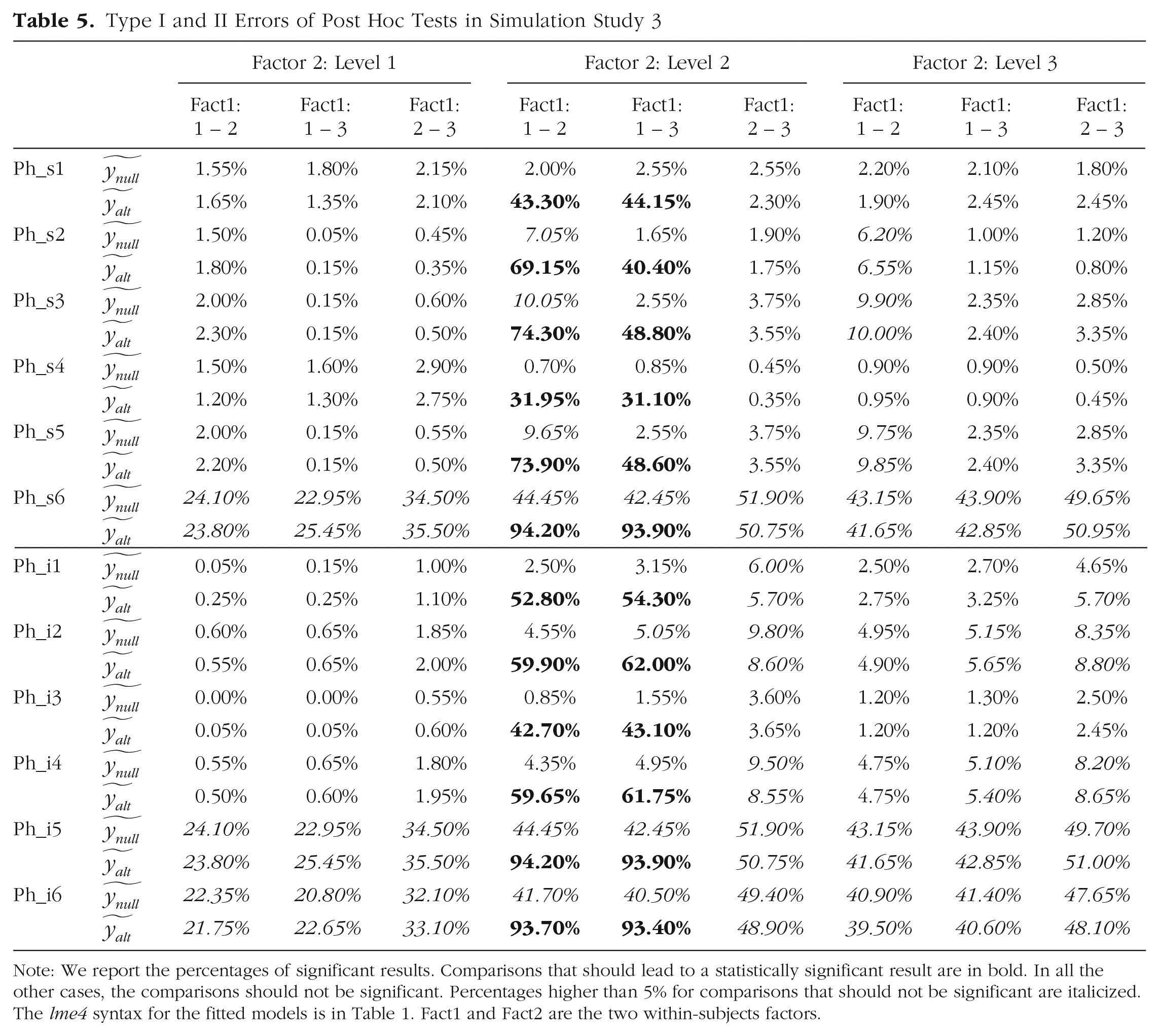
Note: We report the percentages of significant results. Comparisons that should lead to a statistically significant result are in bold. In all the other cases, the comparisons should not be significant. Percentages higher than 5% for comparisons that should not be significant are italicized. The lme4 syntax for the fitted models is in Table 1. Fact1 and Fact2 are the two within-subjects factors.

A Step-by-Step Procedure for Efficient and Reliable Random-Effects Structures

Preliminary considerations

In the previous simulations, we showed that full CRI models can lead to the presence of nonidentifiable random intercepts (i.e., a random intercept with zero variance). Nonetheless, the presence of nonidentifiable random intercepts did not affect (a) the estimation of fixed effects (see Supplementary Table in SM2 in the Supplemental Material, in which the range of the standard deviation in the estimation error is between 5.68E-15 and 3.32E-10), (b) the power of the model (see Table 2, in which the full CRI and full random-slopes models have a mean power of 88% and 66%, respectively), (c) the Type I error (see Table 2, in which the full CRI and the full random-slopes models have a Type I error mean of 6.26% and 3.58%, respectively), or (d) the Type I error on post hoc tests based on estimated marginal means (the full CRI model has only three comparisons in which the error is greater than 5% and the magnitude is equal or lower than 6%). Moreover, full CRI models showed lower singularity or convergence issues, reduced time to fit and estimate the ANOVA-like tables with Kenward-Roger degrees of freedom, and lower RAM usage than either the full random-slopes models or full random-slopes models with the correlation matrix of random effects constrained to zero (see Table 3).

Nonetheless, starting with a maximal random-slopes structure is recommended because it has the best trade-off between Type I and Type II errors. Main effects and interactions of interest varying within subjects and stimuli should be considered as fixed and random effects (Brauer & Curtin, 2018). LMM users should start with a maximal random-slopes model (Barr et al., 2013), following the best practice guidelines of these approaches, avoiding pseudoreplication and overestimation of degrees of freedom (Barr et al., 2013; Brown, 2021; Matuschek et al., 2017).

However, scholars who may obtain singularity or convergence issues after fitting an uncorrelated maximal model may be tempted to remove the highest-order random effect with the lowest estimated variance. We showed that such models dramatically increase Type I error. In other words, removing within-subjects random slopes increases the risk of overestimating the degrees of freedom and the risk of deflated errors of the fixed-effects estimates.

Here, we make a step forward to avoid the inflation of Type I errors when singularity and convergence issues may arise and propose a step-by-step rationale to select the LMM random-effects structure using CRI (Fig. 1).

Fig. 1.

The procedure to use linear mixed models and complex random intercepts. Process and decision boxes are for explanatory purposes. See the main text for full details on how to implement model reduction.

Model reduction from full CRI models

This pipeline can be applied when full random-slopes models are not feasible or when the access to adequate computational resources is not possible. Other elements of great importance, such as controlling for the normality of both model residuals and random-effects distributions, are not among the present work’s purposes. However, the scripts available online (https://osf.io/zbkdv/) provide the necessary functions to check the selected model’s appropriateness successfully.

Step 1: defining full CRI models

When random-slopes techniques fail in fitting a maximal model, a full CRI model should be considered and defined. CRIs should cover all main effects and interaction, varying within subjects and stimuli. Note that relevant covariates that may not be equally distributed among groups or participants (e.g., the scaled trial number for each observed case) may be considered as fixed effects. Although we did not simulate models with continuous covariates that change across the data, researchers may consider including covariates as random slopes of the CRI that they find the most appropriate. For example, scaled trial number may affect any experimental condition; in our examples, “1 + Trial_Number | Participants:Fact1:Fact2” if the number of the trials restarts each level of Factor 1 and Factor 2 or “1 + Trial_Number | Participant” if the number of the trials does not restart along the experiment. Obviously, it is not possible to use a continuous covariate as random intercept or grouping variable. The model should then be checked for singularity (Step 2) and convergence (Step 3).

Step 2: model singularity

The model can now be run to test for singularity. In case the model is not singular, no action is required, and you can move to Step 3. Otherwise, CRIs with the lowest variance can be removed. We suggest removing one CRI at a time. This step is executed iteratively until a nonsingular model is fitted (for further details, see the Recommendations section).

Step 3: model convergence

At this stage, you should check model convergence. If the model converges, no action is required, and you can move to Step 4. If it does not converge, an appropriate optimization algorithm should be added to the model specification (for a list of other remedies for convergence issues, see Brauer & Curtin, 2018), and the optimized model should be checked again for singularity (i.e., go back to Step 2). If convergence is not reached after the optimization procedures, a simplification of the random structure of the model may be required as outlined in Step 2, and the reduced model should be checked again for singularity (i.e., go back to Step 2).

Step 4: checking the final model

At this stage, with a nonsingular and convergent model, you need to check the distribution of the residuals of the random effects and of the final model. If residuals appear normally distributed, no action is required, and you can move to Step 5. If residuals are not normally distributed, scholars can transform their data and start the pipeline again (i.e., go back to Step 1) or achieve a normal distribution of the residuals by removing influential cases before moving to Step 5.

Step 5: computing ANOVA tables for LMMs

Now that you have the final model, you can compute the F and p values using the Kenward-Roger degrees-of-freedom approximation (especially for small sample sizes). Assuming that you had to simplify the model and given that simplifications may increase Type I error, if an effect is found to be significant but its CRI is not specified in the random structure, the scholar discussing such result should support the analyses by fitting a new LMM with the observed significant effect as CRI in the random structure. In the rare event the new LMM presents some singularity or convergence issues, we advise scholars to report both analyses and discuss discordant results. This should control for the risk of pseudoreplication because CRIs of main effects do not correct for Type I error inflation of interactions (see Models s3 and i2, in which only main effects were part of the random structure and had higher Type I error than Models s1, i1, and i3 models in Simulation Study 1).

Step 6: final model fit and post hoc analyses

After computing p values, you should compute the marginal and conditional coefficients of determination (R²) of the final model (Johnson, 2014; Nakagawa et al., 2017; Nakagawa & Schielzeth, 2013). Marginal and conditional R² values range between 0 and 1 and represent a measure of the proportion of variance accounted by the final model. Whereas the marginal R² values are associated with fixed effects, the conditional R² is associated with fixed and random effects. R² values can be computed via the MuMIn (Barton, 2020) or the performance (Lüdecke et al., 2020) packages, among others. Having a model representing the data, without exceeding in overfitting, is always important, and it becomes critical if the researcher plans to compute post hoc analysis on the model’s estimated marginal means. In other words, if the goodness of fitness is poor, then the mathematical model fitted by the LMM cannot be a good representation of the actual data. This might cause misleading results in the post hoc analysis based on estimated marginal means. Therefore, having a conditional R² greater than .6 (Faraway, 2002) might indicate a model representative of the dependent variable without overfitting and be viable for post hoc analyses on estimated model effects. If the conditional R² is low (e.g., < .6; Faraway, 2002), we advise the scholar to support further the results by performing pairwise comparisons on aggregated data and not to rely exclusively on estimated-marginal-means techniques. In both cases, multiple comparisons should be adequately corrected to reduce the risk of Type I error inflation because of multiple comparisons. Note that although we propose a range of R² values to assess model goodness, this range needs to be taken with caution. The same R² value can be interpreted as adequate or inadequate depending on the nature of the experiment, the variability of the dependent variable, and the purposes of the analysis. For example, if the dependent variable is very noisy and the number of observations is high, a low R² might be considered adequate.

Simulation Study 4: Testing the Proposed Pipeline

To test the efficacy of our proposed pipeline, we simulated data of a 3 × 3 RM design with 30 participants, a homogeneous residual standard deviation of the fixed and random effects (SDs = 60 and 7, respectively), and lowly correlated random effects (r = .2). This was necessary to increase the number of singularity or convergency issues for full CRI models (for further details about model specification, see the Supplemental Material). Each simulated data set was analyzed with a full CRI model, a minimal model with participant-only random intercept, and the reduced full CRI model following Step 2 and Step 3 of the proposed pipeline.

Table 6 shows that our setting created singularity issues (> 15%) in the full CRI model, although in both the minimal and the reduced CRI models, there were no convergence or singularity issues. Crucially, although the minimal model showed extremely large Type I error, the reduced and the full CRI models did not show Type I error inflation for main effects or the interaction.

Table 6.

Type I Error, Power, and Statistics for Each Model in Simulation Study 4

Model	Effect	Type I error	Power	Singularity	Convergence Issues
Full CRIy ≈ Fact1 × Fact2 + (1\|ID) + (1\|ID:Fact1) + (1\|ID:Fact2) + (1\|ID:Fact1:Fact2)	Fact1	5.10%
	Fact2	5.78%		16.98%	0.18%
	Fact1: Fact2	3.55%	82.15%
Reduced CRIy ≈ Fact1 × Fact2 + variable random structure	Fact1	5.10%
	Fact2	5.78%		0.00%	0.00%
	Fact1: Fact2	3.65%	82.15%
Minimal modely ≈ Fact1 × Fact2 + (1\|ID)	Fact1	21.95%
	Fact2	22.25%		0.00%	0.00%
	Fact1: Fact2	6.65%	88.85%

Note: We report the statistics for the maximum full CRI model (Model i1), the reduced full CRI model using the proposed pipeline, and the minimal model (Model Ph_i6). For each model, we report the Type I error for each fixed effect, the power for the interaction, and the percentages of singular and nonconvergent models. Fact1 and Fact2 are the two within-subjects factors. CRI = complex random intercept.

Simulation Study 5: Simulations From Matuschek et al. (2017) Scripts

To ensure that the low Type I error observed above was not a specific case of our simulated data sets, we used the scripts from Matuschek et al. (2017) and specified a two-level categorical fixed effect C with S and I as participants and items grouping factors, respectively (50 participants, 20 items). Further details concerning the simulations are available in Matuschek et al.

We simulated 2,000 data sets with the beta for the null-hypothesis and the alternative-hypothesis populations identical to the original article ( $\overset{͠}{y_{null}}$ with β = [2,000, 0], $\overset{͠}{y_{alt}}$ with β = [2,000, 25]). For each simulation, we fitted all five models as detailed in the original article, a full CRI model, and a model obtained from automatically reducing the full CRI model following our pipeline (see Table 7).

Table 7.

Type I Error, Power, Statistics for Each Model in Simulation Study 5

Model syntax	Description	Type I error	Power	Singularity	Convergence Issues
y ≈ 1 + C + (C\|S) + (C\|I)	Full-slopes model	2.10%	32.30%	79.93%	5.83%
y ≈ 1 + C + (C\|\|S) + (C\|\|I)	Full-slopes model with uncorrelated random slopes	2.35%	33.30%	75.23%	5.15%
y ≈ 1 + C + (C\|\|S) + (1\|I)	Uncorrelated random slopes for the S and only the random intercept of I	3.00%	42.10%	49.10%	4.73%
y ≈ 1 + C + (1\|S) + (C\|\|I)	Uncorrelated random slopes for the I and only the random intercept of S	2.75%	37.10%	52.88%	2.73%
y ≈ 1 + C + (1\|S) + (1\|I)	Only the random interceptsof S and I	3.85%	47.10%	0.00%	0.13%
y ≈ 1 + C + (1\|S) + (1\|S:C) + (1\|I) + (1\|I:C)	Full CRI model	2.35%	33.30%	77.50%	1.48%
y ≈ 1 + C + Variable random structure	Reduced full CRI model	2.55%	36.45%	0.00%	0.03%

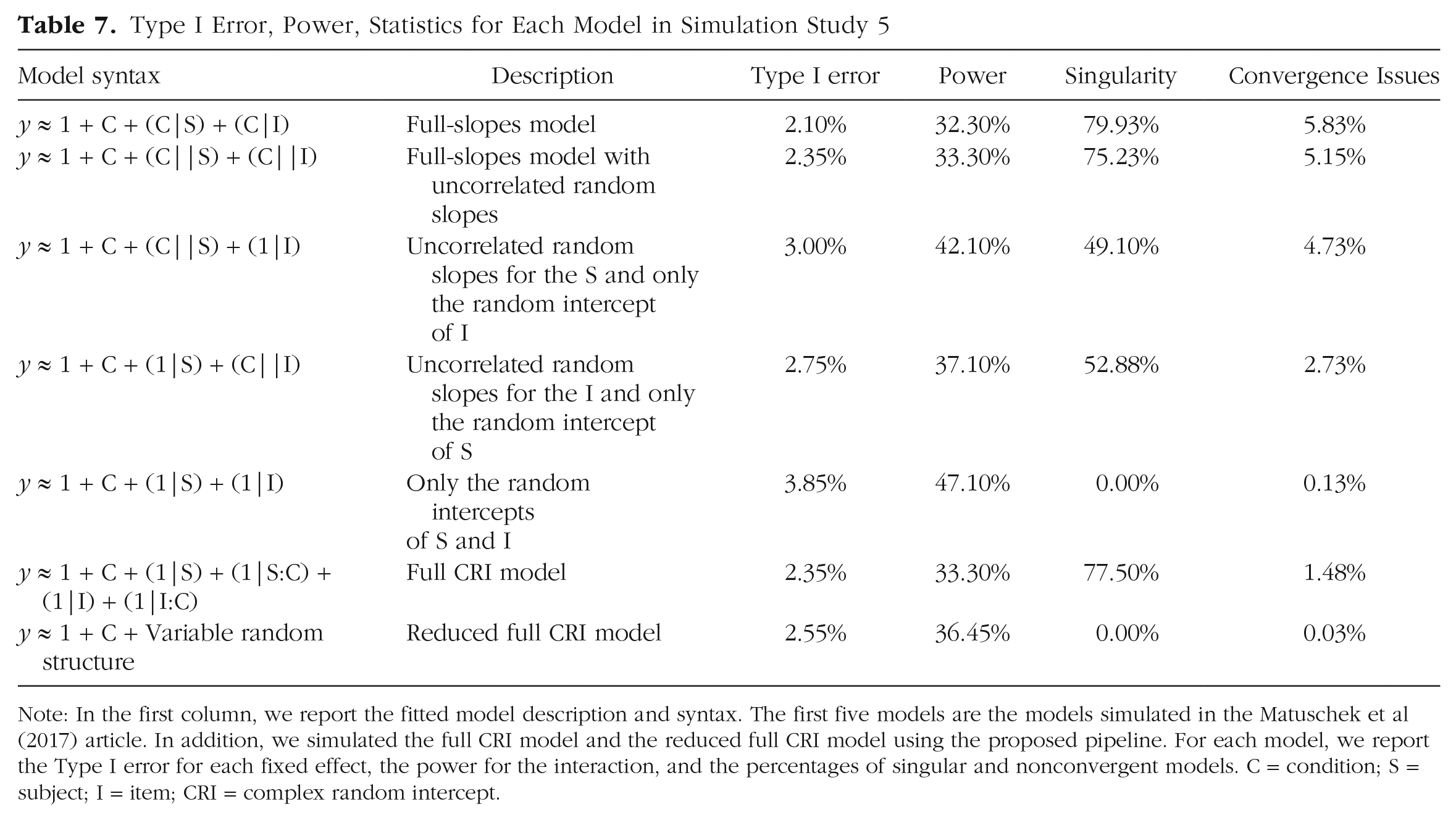
Note: In the first column, we report the fitted model description and syntax. The first five models are the models simulated in the Matuschek et al (2017) article. In addition, we simulated the full CRI model and the reduced full CRI model using the proposed pipeline. For each model, we report the Type I error for each fixed effect, the power for the interaction, and the percentages of singular and nonconvergent models. C = condition; S = subject; I = item; CRI = complex random intercept.

Results in Table 7 show that full-slope, full-slope with uncorrelated random effects, and full CRI models had the highest number of singularities and the lowest Type I error. In this case, the minimal models showed a good Type I error and power, as already shown in Matuschek et al. (2017). This is probably caused by the fact that the simulated experimental design is relatively simple (only one independent variable with two levels: a situation that barely occurs in experimental psychology and neuroscience) and that this minimal model also contains the intercept for each stimulus, an aspect that might limit the pseudoreplication effect by explaining more variability of the data.

Note that the reduced CRI model performed very well and had Type I error and power comparable with the other models and lower converge and singularity issues.

Reanalysis of Singmann and Klauer (2011, Experiment 2)

To further assess the reliability of CRIs, we reanalyzed the sk2011.2 data set available in the afex package (Singmann et al., 2020). The study was a mixed design with one between-subjects factor (instruction) and two within-subject factors (inference, type). Here, we analyzed the dependent variable response with LMM ANOVA tables (see Table 8a), and we tested models that differed in their random structure but not their fixed effects (the scripts are available in the OSF (https://osf.io/zbkdv/) “Reanalyses” folder). Specifically, we compared the results obtained by (a) the maximal model (Model s1), (b) the maximal model without correlations among random effects (Model s2), (c) the model obtained from buildmer (using the method described for Model o1), (d) a full CRI model (Model i1), (e) the model reduced using the proposed pipeline starting from the full CRI model, and (f) a participants’ random-intercept-only model.

Table 8.

ANOVA Tables and Post Hoc Analysis on Real Data

(a) Model number and model random structure
	Maximal model (Model s1)(1 + INFERENCE × TYPE \| ID)		Maximal model without correlations (Model s2)(1 + INFERENCE × TYPE \|\| ID)		Buildmer model (Model o1)(1 + INFERENCE \| ID)		Full CRI model (Model i1)(1 \| ID) + (1 \| ID:INFERENCE) + (1 \| ID:TYPE) + (1 \| ID:INFERENCE:TYPE)		Reduced model(1 \| ID:INFERENCE) + (1 \| ID:INFERENCE:TYPE)		Intercept-only model(1 \| ID)
Is the model nonsingular?					✓				✓		✓
Does the model converge?	✓		✓		✓		✓		✓		✓
ANOVA	df	p	df	p	df	p	df	p	df	p	df	p
(Intercept)	1, 61	.000*	1, 61	.000*	1, 61	.000*	1, 61	.000*	1, 122	.000*	1, 61	.000*
INSTRUCTION	1, 61	.747	1, 61	.745	1, 61	.745	1, 61	.752	1, 122	.751	1, 61	.745
INFERENCE	1, 61	.000*	1, 61	.000*	1, 61	.000*	1, 61	.000*	1, 122	.000*	1, 1061	.000*
TYPE	2, 60	.000*	2, 84.1	.000*	2, 1000	.000*	2, 122	.000*	2, 244	.000*	2, 1061	.000*
INSTRUCTION:INFERENCE	1, 61	.000*	1, 61	.000*	1, 61	.000*	1, 61	.000*	1, 122	.000*	1, 1061	.000*
INSTRUCTION:TYPE	2, 60	.063	2, 84.1	.037*	2, 1000	.033*	2, 122	.060	2, 244	.058	2, 1061	.074
INFERENCE:TYPE	2, 60	.000*	2, 83.5	.000*	2, 1000	.000*	2, 122	.000*	2, 244	.000*	2, 1061	.000*
INSTRUCTION:INFERENCE:TYPE	2, 60	.031*	2, 83.5	.017*	2, 1000	.001*	2, 122	.002*	2, 244	.002*	2, 1061	.003*
(b) Post hoc analysis of INSTRUCTION:INFERENCE:TYPE
Estimates, M ± SD	1.699 ± 29.651		1.699 ± 29.651		1.699 ± 29.651		1.699 ± 29.651		1.699 ± 29.651		1.699 ± 29.651
Estimates, SE ± SD	5.337 ± 1.130		5.225 ± 0.772		5.014 ± 1.071		5.184 ± 0.753		5.184 ± 0.753		4.300 ± 0.477
Bonferroni-corrected p < .05 out of 66 comparisons	40		39		41		39		39		42

Note (a) Each column represents a model and whether it was a nonsingular and convergent model. Each row represents a predictor of the model, and we report the degrees of freedom and p values obtained from the different linear mixed models. For simplicity, each model’s label indicates how the random-effects structure has been adapted based on Models s1, s2, o1, and i1; a reduced model using the proposed pipeline; and an intercept-only model. (b) We report a descriptive evaluation of the triple instruction:inference:type interaction for each model. We show the average of the estimates (±SD), the average standard error of the estimates (±SD), and the total number of significant Bonferroni-corrected comparisons for that model. ANOVA = analysis of variance.

p < .05.

We collected convergence and singularity issues, degree of freedom, and p-value estimates for each model. Models were fitted using afex (Version 1.1-1; Singmann et al., 2020), lme4 (Version 1.1-29; Bates et al., 2015), and buildmer (Version 2.4; Voeten, 2022). The p values were computed using Kenward-Roger degrees of freedom with the R package car (Version 3.0-13; Fox & Weisberg, 2019). All these analyses were carried out in R (Version 4.1.2; R Core Team, 2018).

All models produced similar results with few exceptions (see Table 8a). In particular, p values of the double instruction:type interaction was significant for the model without correlations and the model obtained from buildmer. Moreover, the triple interaction instruction:inference:type was significant in all models. Thus, we explored whether multiple comparisons of this interaction were affected by different random structures (see Table 8b). Results indicate that the model with the participants’ intercept only was the most anticonservative with 42 out of 66 Bonferroni-corrected paired comparisons showing a p value lower than .05, followed by the model obtained by buildmer. Note that the reduced model following our suggested pipeline had no convergence and singularity issues, and both ANOVAs and Bonferroni-corrected paired comparisons were highly similar to the full random-slopes model. Overall, these reanalyses support the importance of including significant effects as CRIs or random slopes and indirectly confirm the findings from the simulation studies.

Discussion

In a series of studies, we tested the reliability of different methods used to reduce overfitted LMMs in fully crossed experimental designs. We showed that removing correlations or random slopes to achieve nonsingular and convergent models may dramatically inflate Type I errors. We also introduced a new method for model reduction using CRI and tested its reliability for hypothesis testing using simulated and real data. Finally, we proposed and tested a pipeline to reduce arbitrary decisions when reducing an overparametrized model and to achieve nonsingular and convergent models without inflating Type I errors.

To the best of our knowledge, our work for the first to show that using CRIs can play an important role in reducing pseudoreplication and obtaining models with few convergence problems. Moreover, it also demonstrates the importance of adding CRIs of significant effects. Our pipeline can be successfully applied following six steps and a few simple criteria to obtain conservative reduced LMMs (see Fig. 1 and A Step-by-Step Procedure for Efficient and Reliable Random-Effects Structures). We combined into a single procedure many suggestions (e.g., use of maximal model, the possibility of simplifying overparametrized models by removing random slope or correlations) put forward by different scholars (Barr, 2013; Barr et al., 2013; Bates et al., 2018; Brauer & Curtin, 2018; Singmann & Kellen, 2020) and extended them by using CRIs.

Note that although we mainly based our results on simulated data for statistical inference, pseudoreplication problems might inflate Type I error also in other statistics influenced by degrees of freedom, such as the Akaike information criterion, or even in statistical procedures that can be independent from degrees of freedom, such as bootstrap techniques. The procedure set out in this article does not have the ambition to be perfect in terms of Type I error and power but, rather, to be a pragmatic approach with a clear and concise step-by-step procedure that can be used by any scholar who wants to use a method validated by simulations with clear recommendations.

Recommendations for model reduction

Scholars usually reduce maximal models to increase the power of LMMs. It is known—and shown also by our simulations—that removing random effects from the random-effects structure can dramatically increase Type I error. Henceforth, scholars who have access to adequate computational resources are recommended to start from a maximal model. In case limited computational resources do not allow computing the model, the p values, or multiple comparisons or unforeseen system errors preclude statical analyses, our pipeline provides the possibility to start from full CRI models. Using CRIs to avoid Type I error inflation also extends other approaches when these may fail to solve singularity and convergence issues (Brauer & Curtin, 2018; Singmann & Kellen, 2020). This may be crucial if the scholar cannot compute the maximal model in the first instance, precluding the possibility to assess which random effects have the lowest variance or whether the model has any singularity/convergence issue. Moreover, our pipeline suggests few clear steps (i.e., starting from a full CRI model and removing CRIs with the lowest variance one at a time) to avoid anticonservative results (e.g., by supporting main findings by also analyzing aggregated data).

Practical implications for statistical inference

In terms of Type I errors and power, the full-random-slopes models (Model s1) have the best performance. However, full CRI models (Model i1) may be a valid alternative to (non)correlated full random-slopes models. That is, scholars may start directly with a full CRI model when there is limited computing power or a small number of data points or when singularity or convergence issues arise. Conversely, the resulting models from automatic packages, such as buildmer, have the advantage to always avoid convergence and singularity issues, but unfortunately, they tend to show higher Type I error.

In this article, we presented a practical step-by-step procedure to simplify the random-effects structure of an LMM while controlling for pseudoreplication. Our approach differs from other approaches because we provide a single criterion to remove random effects (i.e., the CRI with the lowest variance), reducing the risk of arbitrary decisions (e.g., removing the highest-order effect or keeping it) and spurious results.

We tested our pipeline in three different ways: two based on data simulations and one using real data. In all cases, the reduced model never inflated Type I error. We also checked the models’ performance in post hoc analyses based on estimated marginal means by using the emmeans package, one of the most used among researchers. We showed that models with a highly reduced random-effects structure will likely increase Type I errors even after applying conservative corrections. Conversely, post hoc tests computed on the estimates of the simplified models following the suggested pipeline did not inflate Type I error and were more conservative.

However, based on our simulations, any model reduction of the random-slopes structure may increase the Type I error compared with a full-slopes maximal model. Thus, scholars should carefully discuss a fixed effect with a significant p value obtained from a reduced model and may also try to validate their findings by analyzing the data in other supportive way (e.g., adding effect sizes and/or confidence intervals). Moreover, note that post hoc testing on the estimated effects of a model with a poor conditional R² may lead to greater Type I errors and biased results. In these cases, it is recommended to compute post hoc testing with pairwise t tests, or pairwise regressions when necessary, on aggregated data and apply family-wise error corrections.

Simulation differences between this work and other studies

Our simulations adopted a frequentist approach and lead to more Type I errors and singularity and convergence issues than the reader can find in other articles based on data simulations. This is because the seminal and traditional simulative approach to validate statistical procedures is to simulate data that perfectly follow all model assumptions and to simulate simple experimental designs to have clearer insights concerning the validity of the proposed approach.

Notwithstanding these methodologies are of the utmost importance and a validation has to use one of such approaches (in this work, we used the simulation scripts from the seminal work of Matuschek et al., 2017), sometimes simulated data are different from the data obtained in real experiments. Moreover, at least from our and other colleagues’ experience, (un)correlated full random-slopes models often lead to nonconvergence or singularity issues, and traditional model-reduction methods lead to pseudoreplication issues.

For all these reasons, we lowered the number of simulated participants under the recommended level (note that we also simulated data with 50 and 30 participants in Simulation Studies 2 and 4, respectively), and we used two categorical independent variables with three levels each. We believe this approach allowed us to simulate more closely a psychology or neuroscience experimental design and allowed us to stress the difficulties in obtaining models with no singularities and convergence issues.

Conclusions

In this article, we proposed transforming random slopes into CRIs to control for Type I error inflation following model reduction. We also proposed a new and concise iterative decision process to determine the random-effects structure starting from a full CRI LMM. We demonstrated that our approach successfully reduces the risk of Type I error inflation by providing a few criteria to interpret results from reduced models. We believe this step-by-step approach can be easily implemented also by scholars and reviewers who are new to LMMs. Moreover, scholars who have not enough computational power or enough observations to start with a full random-slopes model can directly start with a full CRI model. Our step-by-step approach, together with other seminal approaches (Barr et al., 2013; Matuschek et al., 2017), may positively contribute to reduce study replication failure, and although we applied this approach to LMMs and behavioral data, we believe our pipeline may also be applied to generalized LMMs and neural data.

Supplemental Material

sj-docx-1-amp-10.1177_25152459231214454 – Supplemental material for Reliability and Feasibility of Linear Mixed Models in Fully Crossed Experimental Designs

Supplemental material, sj-docx-1-amp-10.1177_25152459231214454 for Reliability and Feasibility of Linear Mixed Models in Fully Crossed Experimental Designs by Michele Scandola and Emmanuele Tidoni in Advances in Methods and Practices in Psychological Science

Footnotes

Acknowledgements

We acknowledge the Viper High Performance Computing facility of the University of Hull and its support team (http://hpc.wordpress.hull.ac.uk/home/). We thank Richard O’Connor for his helpful insights on an earlier version of the article. The codes used for the simulations are available online ().

Transparency

Action Editor: Rogier Kievit

Editor: David A. Sbarra

Author Contributions

Authors are listed in alphabetical order. Both authors contributed equally.

Michele Scandola: Conceptualization; Data curation; Formal analysis; Investigation; Methodology; Project administration; Resources; Software; Validation; Visualization; Writing – original draft; Writing – review & editing.

Emmanuele Tidoni: Conceptualization; Data curation; Formal analysis; Investigation; Methodology; Project administration; Resources; Software; Validation; Visualization; Writing – original draft; Writing – review & editing.

ORCID iD

Emmanuele Tidoni

Supplemental Material

Additional supporting information can be found at

Notes

References

Baayen

R. H.

Davidson

D. J.

Bates

D. M.

(2008). Mixed-effects modeling with crossed random effects for subjects and items. Journal of Memory and Language, 59(4), 390–412. https://doi.org/10.1016/j.jml.2007.12.005

Barr

D. J.

(2013). Random effects structure for testing interactions in linear mixed-effects models. Frontiers in Psychology, 4, Article 328. https://doi.org/10.3389/fpsyg.2013.00328

Barr

D. J.

Levy

Scheepers

Tily

H. J.

(2013). Random effects structure for confirmatory hypothesis testing: Keep it maximal. Journal of Memory and Language, 68(3), 255–278. https://doi.org/10.1016/j.jml.2012.11.001

Barton

(2020). MuMIn: Multi-model inference (R Package Version 1.43.17). https://CRAN.R-project.org/package=MuMIn

Bates

(2010). Lme4: Mixed-effects modelling with R. https://people.math.ethz.ch/~maechler/MEMo-pages/lMMwR.pdf

Bates

Kliegl

Vasishth

Baayen

(2018). Parsimonious mixed models. ArXiv. https://doi.org/10.48550/arXiv.1506.04967

Bates

Mächler

Bolker

Walker

(2015). Fitting linear mixed-effects models using lme4. Journal of Statistical Software, 67(1), 1–51. https://doi.org/10.18637/jss.v067.i01

Brauer

Curtin

J. J.

(2018). Linear mixed-effects models and the analysis of nonindependent data: A unified framework to analyze categorical and continuous independent variables that vary within-subjects and/or within-items. Psychological Methods, 23(3), 389–411. https://doi.org/10.1037/met0000159

Brown

V. A.

(2021). An introduction to linear mixed-effects modeling in R. Advances in Methods and Practices in Psychological Science, 4(1), 2515245920960351.

10.

Brysbaert

Stevens

(2018). Power analysis and effect size in mixed effects models: A tutorial. Journal of Cognition, 1(1), Article 9. https://doi.org/10.5334/joc.10

11.

Crawley

M. J.

(2012). The R book. John Wiley. https://doi.org/10.1002/9781118448908

12.

DeBruine

L. M.

(2021). Faux: Simulation for factorial designs. Zenodo. https://doi.org/10.5281/zenodo.2669586

13.

DeBruine

L. M.

Barr

D. J.

(2021). Understanding mixed-effects models through data simulation. Advances in Methods and Practices in Psychological Science, 4(1). https://doi.org/10.1177/2515245920965119

14.

Faraway

(2002). Practical regression and ANOVA using R. http://cran.r-project.org/doc/contrib/Faraway-PRA.pdf

15.

Fox

Weisberg

(2019). An R companion to applied regression (3rd ed.). Sage.

16.

Gelman

Carlin

(2014). Beyond power calculations: Assessing Type S (Sign) and Type M (Magnitude) errors. Perspectives on Psychological Science, 9(6), 641–651. https://doi.org/10.1177/1745691614551642

17.

Gelman

Hill

(2006). Data analysis using regression and multilevel/hierarchical models. Cambridge University Press. https://doi.org/10.1017/CBO9780511790942

18.

Harrison

X. A.

Donaldson

Correa-Cano

M. E.

Evans

Fisher

D. N.

Goodwin

C. E. D.

Robinson

B. S.

Hodgson

D. J.

Inger

(2018). A brief introduction to mixed effects modelling and multi-model inference in ecology. PeerJ, 6, Article e4794. https://doi.org/10.7717/peerj.4794

19.

Hothorn

Bretz

Westfall

(2008). Simultaneous inference in general parametric models. Biometrical Journal, 50(3), 346–363. https://doi.org/10.1002/bimj.200810425

20.

Johnson

P. C. D.

(2014). Extension of Nakagawa & Schielzeth’s R 2 GLMM to random slopes models. Methods in Ecology and Evolution, 5(9), 944–946. https://doi.org/10.1111/2041-210X.12225

21.

Judd

C. M.

Westfall

Kenny

D. A.

(2012). Treating stimuli as a random factor in social psychology: A new and comprehensive solution to a pervasive but largely ignored problem. Journal of Personality and Social Psychology, 103(1), 54–69. https://doi.org/10.1037/a0028347

22.

Kuznetsova

Brockhoff

P. B.

Christensen

R. H. B.

(2017). lmerTest package: Tests in linear mixed effects models. Journal of Statistical Software, 82(13), 1–26. https://doi.org/10.18637/jss.v082.i13

23.

Lenth

(2023). emmeans: Estimated marginal means, aka least-squares means (R Package Version 1.8.9). https://cran.R-project.org/package=emmeans

24.

Lenth

Singmann

Love

Buerkner

Herve

(2020). Estimated marginal means, aka least-squares means (R Package Version 1.5.0). https://cran.r-project.org/web/packages/emmeans/emmeans.pdf

25.

Lüdecke

Makowski

Waggoner

Patil

(2020). Performance: Assessment of regression models performance (R Package Version 0.4.6). https://CRAN.R-project.org/package=performance

26.

Luke

S. G.

(2017). Evaluating significance in linear mixed-effects models in R. Behavior Research Methods, 49(4), 1494–1502. https://doi.org/10.3758/s13428-016-0809-y

27.

Matuschek

Kliegl

Vasishth

Baayen

Bates

(2017). Balancing Type I error and power in linear mixed models. Journal of Memory and Language, 94, 305–315. https://doi.org/10.1016/j.jml.2017.01.001

28.

Meteyard

Davies

R. A. I.

(2020). Best practice guidance for linear mixed-effects models in psychological science. Journal of Memory and Language, 112, Article 104092. https://doi.org/10.1016/j.jml.2020.104092

29.

Nakagawa

Johnson

P. C. D.

Schielzeth

(2017). The coefficient of determination R 2 and intra-class correlation coefficient from generalized linear mixed-effects models revisited and expanded. Journal of the Royal Society Interface, 14(134), Article 20170213. https://doi.org/10.1098/rsif.2017.0213

30.

Nakagawa

Schielzeth

(2013). A general and simple method for obtaining R 2 from generalized linear mixed-effects models. Methods in Ecology and Evolution, 4(2), 133–142. https://doi.org/10.1111/j.2041-210x.2012.00261.x

31.

Pinheiro

J. C.

Bates

D. M.

(2000). Mixed-effects models in S and S-PLUS. Springer-Verlag. https://doi.org/10.1007/b98882

32.

R Core Team. (2018). R: A language and environment for statistical computing. https://www.r-project.org/

33.

Singmann

Bolker

Westfall

Aust

Ben-Shachar

M. S.

(2020). Afex: Analysis of factorial experiments (R Package Version 0.27-2). https://CRAN.R-project.org/package=afex

34.

Singmann

Kellen

(2020). An introduction to mixed models for experimental psychology. In Spieler

Schumacher

(Eds.), New methods in cognitive psychology (pp. 4–31). Routledge. https://doi.org/10.4324/9780429318405-2

35.

Singmann

Klauer

K. C.

(2011). Deductive and inductive conditional inferences: Two modes of reasoning. Thinking & Reasoning, 17(3), 247–281. https://doi.org/10.1080/13546783.2011.572718

36.

Stroup

W. W.

(2012). Generalized linear mixed models: Modern concepts, methods and applications. CRC Press. https://doi.org/10.1201/b13151

37.

Voeten

C. C.

(2022). Buildmer: Stepwise elimination and term reordering for mixed-effects regression (R Package Version 2.3). https://CRAN.R-project.org/package=buildmer

Supplementary Material

Please find the following supplemental material available below.

For Open Access articles published under a Creative Commons License, all supplemental material carries the same license as the article it is associated with.

For non-Open Access articles published, all supplemental material carries a non-exclusive license, and permission requests for re-use of supplemental material or any part of supplemental material shall be sent directly to the copyright owner as specified in the copyright notice associated with the article.

0.00 MB

0.02 MB