Sage Journals: Discover world-class research

Abstract

Scientific theories explain phenomena using simplifying assumptions—for instance, that the speed of light does not depend on the direction in which the light is moving, or that the shape of a pea plant’s seeds depends on a small number of alleles randomly obtained from its parents. These simplifying assumptions often take the form of statistical null hypotheses; hence, supporting these simplifying assumptions with statistical evidence is crucial to scientific progress, though it might involve “accepting” a null hypothesis. We review two historical examples in which statistical evidence was used to accept a simplifying assumption (that there is no luminiferous ether and that genetic traits are passed on in discrete forms) and one in which the null hypothesis was not accepted despite repeated failures (gravitational waves), drawing lessons from each. We emphasize the role of the scientific context in acceptance of the null: Accepting a null hypothesis is never a purely statistical affair.

Keywords

hypothesis testing null hypothesis history of science philosophy of science statistics open data open materials

On a warm summer morning in 1887, Albert Michelson hunched over a heavy stone table in a basement of Western Reserve College. He peered through an eyepiece whose other end disappeared under a wooden hood covering the table. With his right hand, he slowly turned a screw to calibrate 1 of 16 mirrors fixed to the stone. Beneath the hood, beams of yellow sodium light bounced back and forth between the mirrors along two perpendicular paths that both ended at the eyepiece. By adjusting the screw, Michelson ensured that the lengths of the two paths were equal.

The stone slab sat on a piece of wood, which itself was floating in a pool of liquid mercury. Around noon, Michelson gave the table a push, causing it to spin slowly. Every 22.5° of rotation—about as many seconds—he looked through the eyepiece and scribbled down a number. That afternoon, he took more than 100 readings, stopping only to give the table a small push to keep it spinning. He came back that evening for another hundred measurements, and repeated the process again over the next 2 days.

The numbers Michelson and his colleague Edward Morley scribbled down in 1887 would eventually be among the most celebrated results in science. What they found—or rather, what they did not find—was a quandary for popular 19th-century theories of light propagation. Michelson and Morley’s (1887) result foreshadowed not one but two revolutions in physics—special relativity and quantum theory—and eventually won Michelson the Nobel Prize in physics.

It has been noted for decades that psychological science largely rests on asserting statistical differences by using null-hypothesis significance tests rather than on understanding sameness, patterns, or regularity (see, e.g., Gigerenzer, Krauss, & Vitouch, 2004; Meehl, 1978; Sterling, Rosenbaum, & Weinkam, 1995). We present three historical vignettes involving acceptance and rejection of null hypotheses in mature sciences. None of these inferences rest on significant differences in null-hypothesis significance tests, but they are nevertheless examples of scientific progress. The first vignette concerns Michelson and Morley’s null result in their experiments on the wave theory of light, the second focuses on Mendel’s famous (and controversial) genetic experiments (Fisher, 1936; Mendel, 1866/1996), and the third concerns the recent Nobel-Prize-winning findings by the Laser Interferometer Gravitational-Wave Observatory (LIGO) team. Understanding how the scientific context can support acceptance of null hypotheses is key to understanding why statistical nulls have often been ignored in psychology.

Kuhnian Paradigms and Normal Science

In The Structure of Scientific Revolutions, Kuhn (1962) offered a generally descriptive account of how all sciences appear to have changed over time. To the extent that these changes can be construed in terms of developmental progress, they follow from motivations that appear to be common among scientific enterprises: motivations to improve understanding of a wide range of phenomena and to provide increasingly specified guides for further scientific research. Kuhn illustrated this general trajectory by identifying two stages of development.

The first of these stages is termed the preparadigm stage, and it is marked by an absence of any unifying perspectives. At this stage, theories proliferate at the pace of observed effects, and these theories are little more than descriptions of phenomena (e.g., when X is placed over a flame, Y occurs). Because these theories offer little regarding underlying mechanisms, they present no clear hypotheses beyond the hypothesis that the original effect can be replicated. They are essentially tautological, reflecting little in the way of general understanding of a phenomenon, and unable to produce novel predictions.

According to Kuhn, all scientific communities eventually acknowledge this limitation and gradually make their way to a standard phase of scientific inquiry. In this normal-science phase, an underlying construct is hypothesized to manifest itself through various previously unrelated empirical phenomena (e.g., space-time or genes). This hypothesized unifying construct lies at the core of a new paradigm, a broad nest of theoretical conceits that shape predictions for future observations. Increasing specificity of the nature of these conceits—theory articulation—guides the identification of novel effects (rather than the generation of novel “theories”) and subsequent research efforts.

Kuhn’s depiction of normal-science progress does not rest on a particular epistemic school of thought. Rather, paradigms are understood to facilitate progress by motivational means, insofar as they represent progress narratives that encourage scientists to predict and accumulate paradigm-verifying effects rather than perseverate on potentially falsifying anomalies (see also the positive heuristic—Lakatos, 1970).

The motivational and verificationist realities of normal science have fundamental implications for how the “null hypothesis” is interpreted, and whether or not it is “accepted.” In a normal-science setting, multiple explanatory paradigms may offer competing accounts of demonstrated effects and differing predictions for what may be observed in the future. When hypotheses following from a given paradigm are not supported by the data, the null hypotheses can be readily accepted, as the observed “null” effects may offer support for competing paradigms and represent additional elements of accumulated knowledge. Alternatively, normal science may be dominated by a single, broad explanatory paradigm that can account for the bulk of prior findings and continues to make successful predictions for demonstrable effects. In this setting, scientists may be extremely reluctant to accept a null hypothesis because it would challenge a paradigm that must be correct, insofar as it has been otherwise verified in dozens (or even hundreds) of prior experiments, and because there are no other options, which means that the acceptance of the null could lead to a scientific crisis.

We next discuss three examples of important inferences drawn from a failure to find deviations from statistical null hypotheses, demonstrated within the paradigmatic context of normal science. The first and the third are from 19th- and 21st-century physics, respectively; the second is from 19th- and 20th-century biology. In each case, we emphasize the relationship of the statistical inference for or against a null hypothesis with the scientific inference in the context of the relevant paradigm. After presenting these examples, we contrast the situation in normal science with that in present-day psychology.

Michelson, Morley, and the Luminiferous Ether

For many centuries, there were two competing theories explaining the behavior of light. Emission theory, championed by Newton, held that light was made up of particles that moved in straight lines called rays. The opposing view, developed by Huygens, held that light was a wave. In the 18th century, the emission view was dominant. Emission theory is perhaps more consistent with everyday observations of light: Light appears to move in straight lines, as a particle would.

In the beginning of the 19th century, the wave theory of light gained the upper hand among physicists as a result of the discovery of interference phenomena. When two waves of different phases meet, they cancel and reinforce one another in complicated patterns. Light behaves this way: When light is forced through two slits, the light from one slit interferes with the light from the other, and vice versa. This forms dark and light bands where the waves cancel and reinforce one another. Interference phenomena cannot be easily explained by an emission theory.

Expectations for light waves were built on experience with other waves that people understood: waves in water or air. If light is a wave, it was reasoned, it must be a wave in some medium. Whatever this medium is, it carries starlight above the Earth and torchlight below it. This medium must be able to pass through solid matter because light moves through glass, and it must exist in a vacuum. Wave theorists gave this mysterious medium a name: the luminiferous ether.

Physicists thought that a sea of luminiferous ether existed throughout space, providing a fixed reference against which everything moved. As the Earth revolved around the Sun, it was passing through the ether. Facts known at the time ruled out the idea that the ether was dragged along with the Earth; hence, the Earth had to be moving through the ether at some speed.

But at what speed? This was the question Michelson and Morley sought to answer. Michelson had invented and refined an ingenious experimental device now known as a Michelson interferometer. The 1887 version is shown in Figure 1, in both perspective and top-down views.

Fig. 1.

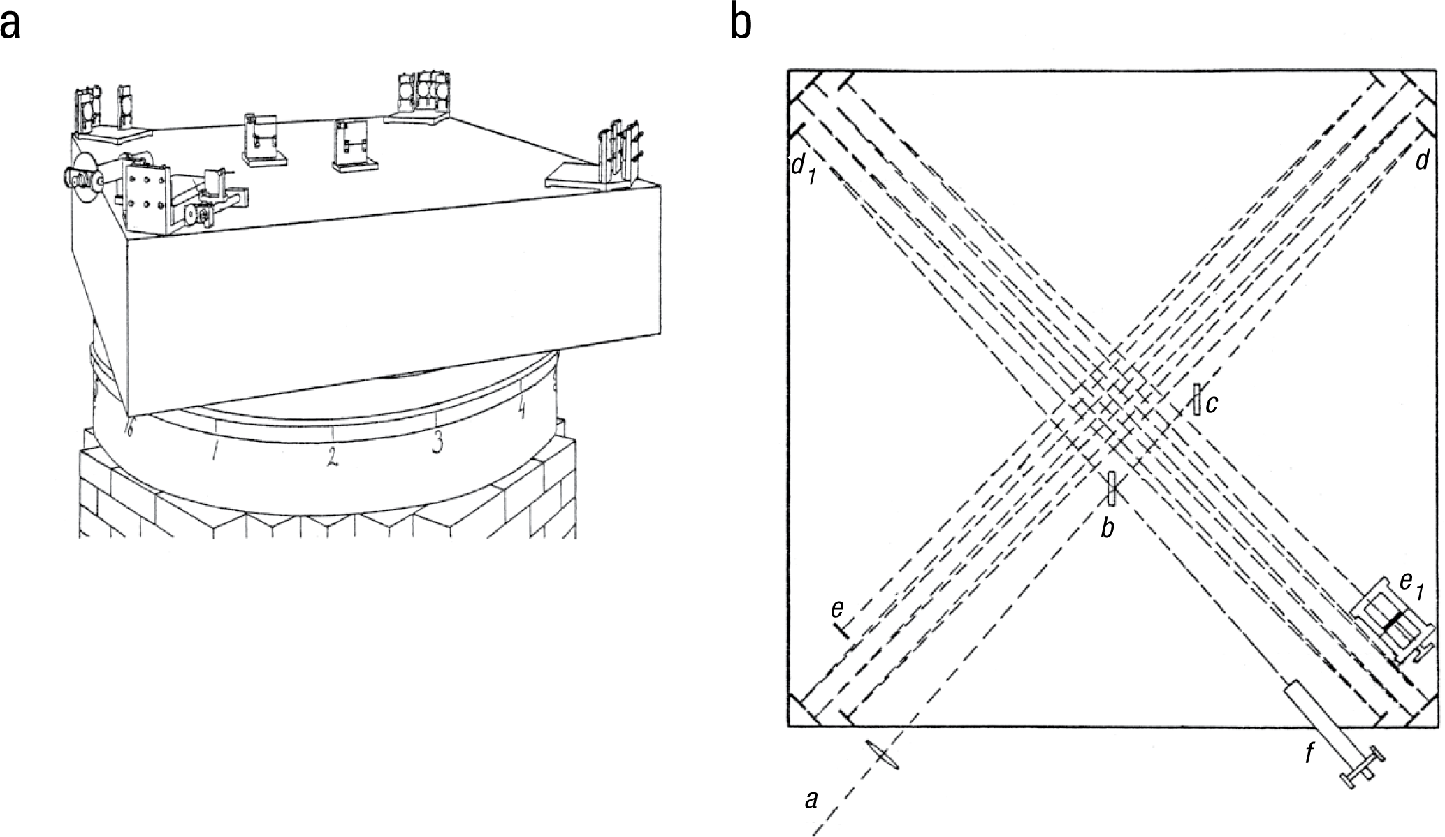
Michelson and Morley’s interferometer: (a) a perspective drawing of the 1.5-m-square device without its wooden cover and (b) a schematic of the table surface. As illustrated in (b), light emitted from the light source, a, passed through a lens and hit a beam splitter, b, which sent the light along one of two perpendicular paths. The light was then reflected back and forth by mirrors at d (first path) and d₁ (second path), until they were reflected back by mirror e (first path) or e₁. (second path). Finally, the two beams passed back though the beam splitter, and part of each beam was sent to an eyepiece, f. The mirror e₁ was finely adjustable so that the two beams could be equated in length. An extra beam splitter, c, was used to ensure that the beams in the two paths moved through the same amount of glass. These illustrations are adapted from Figures 3 and 4 in Michelson and Morley (1887) and are in the public domain.

The basic idea behind Michelson’s interferometer is that light comes from a common source and is focused by a lens. The light is then split and sent along two perpendicular paths; each beam bounces back and forth between sets of mirrors. A final mirror along each path sends each beam back the way it came. The beams are then recombined and pass to an eyepiece. The lengths of the two perpendicular paths can be made equal by carefully adjusting a mirror along one of the paths.

When Michelson looked into the eyepiece while he was sending white light into the interferometer, he saw a pattern of vertical dark and light bands, called “fringes,” formed by interference between the various components of the white light. Michelson and Morley reasoned that by rotating the stone table on which the interferometer was set, they were manipulating how the two paths of light were moving with respect to the “wind” created by the Earth’s—and thus the device’s—movement through the ether. At some point in the rotation, one path would be parallel to the direction of the wind, and the other would be perpendicular to it; at another point, the opposite relations to the wind would obtain.

The theory held that light moved with the ether, but the interferometer itself moved with the Earth. Therefore, if one path was moving parallel to the ether wind and the other was moving perpendicular to it, the light beams in the two paths moved different distances with respect to the ether. Any difference between the distances traveled by the light in the two paths would cause the interference fringes to shift to one side by an amount that depended on the speed of the Earth’s motion through the ether. Given that the speed of the Earth in its orbit is 30 km per second, Michelson and Morley expected the fringes to shift by a maximum of 0.4 fringe widths. This maximum shift would occur when one path was facing into the ether wind and the other was perpendicular to it. The minimum expected shift was 0, when the two paths faced into the ether wind at the same angle (see the schematic at the top of Fig. 2).

Fig. 2.

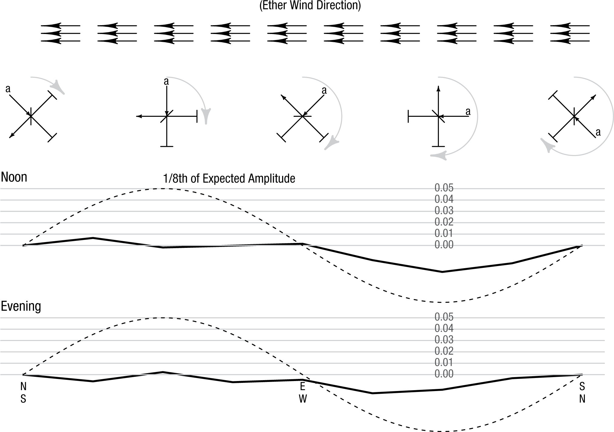
The observed fringe shift from Michelson and Morley’s experiment, as presented in their 1887 article. The data have been detrended to remove the subtle effects of temperature changes throughout the day. The top series shows the average for the noon runs, and the bottom series shows the average for the evening runs. The y-axis is the amount of shift, in fringes. Also shown (dashed curves) is the expected pattern at 1/8 the expected amplitude of 0.4. The schematic above the series shows the hypothesized direction of the ether wind and the position of the interferometer with respect to the wind at five points during each series; the point marked “a” represents the light source on the sketch of the instrument (see Fig. 1). “N,” “S,” “E,” and “W” at the bottom of the figure refer to the cardinal directions and represent where the apparatus was facing at that point in the rotation. This figure is licensed under CC BY 4.0.

Michelson (or Morley) gave the table a slow but steady spin and measured the shift at 16 rotation angles, which worked out to once every 23 s. They repeated the process consecutively five times, for a total of six rotations, at noon and then six times again in the evening, on three different days. The fringe-shift measurements were detrended to remove the effects of ambient temperature changes and then averaged. Michelson and Morley expected the data to follow a sine curve with amplitude of 0.4 fringe widths; Figure 2 shows what they found.

There does not appear to be any discernible relationship between the angle of the table’s rotation and the fringe shift. There was so little effect relative to the expected shifts that Michelson and Morley’s figure depicting their results did not show the expected effect for purposes of comparison; the maximum value in their figure was only 1/8th of the predicted value, because if the range of the y-axis had extended to the predicted value, all the variability in the data would have been hidden. Despite the smallness of the observed effect, Michelson and Morley (1887) did not directly “accept” the null hypothesis that there was no relationship between the angle and the fringe shift. Instead, they said that

The displacement to be expected was 0.4 fringe. The actual displacement was certainly less than the twentieth part of this, and probably less than the fortieth part. But since the displacement is proportional to the square of the velocity, the relative velocity of the earth and the ether is probably less than one sixth the earth’s orbital velocity, and certainly less than one-fourth. . . . It appears, from all that precedes, reasonably certain that if there be any relative motion between the earth and the luminiferous ether, it must be small. . . . (p. 341)

This conclusion was subject to continued investigation for decades, using more precise interferometers and at different times of the year. For example, a recent replication by Eisele, Nevsky, and Schiller (2009) used an interferometer 100 million times as precise as Michelson and Morley’s device. The result was still null. Michelson and Morley are remembered as having established that there is no ether, but why is their result considered convincingly null, given that they merely reported an upper bound on the possible speed of the Earth moving through the ether? We suggest that there are four reasons:

The experiment was highly sensitive: Michelson and Morley’s 1887 experiment was actually the second such experiment for which Michelson published a report. In 1881, he presented results that were similar, but obtained using a device that was 1/10th as sensitive.¹ Other researchers noted that even before accounting for a calculation mistake, “[the fringe shift] to be measured . . . was already barely beyond the limits of the errors of [the 1881] experiment” and hence “the conclusion drawn . . . might well be questioned” (Michelson & Morley, 1887, p. 335). Thankfully, the 10-fold increase in sensitivity in 1887 was made possible by a clever arrangement of mirrors. The resulting high sensitivity made for a more convincing null result.

A parametric manipulation was used: When researchers discuss null results in psychology, they often refer to a single effect that is not statistically significant. Michelson and Morley, however, were looking for a data pattern, rather than a single effect. The sine wave pattern expected to result from the rotation of the table—a parametric manipulation of the size of the expected effect—did not present itself. The test of the theory was therefore much stronger than it would have been if only one rotational angle had been considered.

The data were tested against a theoretical expectation: The speed of the Earth moving around the Sun provided a value against which the null result could be compared. Michelson and Morley admitted that it was possible that motions other than the Earth moving around the Sun—for instance, the Sun moving through the galaxy—might have come into play, but to get the null result, these motions would all have had to add up just right to cancel out. This would have been quite the coincidence, so Michelson and Morley concluded that “chances are much against it” (p. 341). They noted, however, that repeating the experiment at longer time intervals would allow testing this possibility.

Competing paradigms were available: As previously mentioned, in the 19th century, the wave theory of light was dominant, but it was not the only theory. The competing emission theory had no need for ether. Emission theory continued to be modified to account for new evidence into the late 19th and early 20th century (e.g., Ritz, 1908/1980). Additionally, neither of the two major 20th-century theories in physics required the luminiferous ether. Einstein’s (1905/2013) special theory of relativity made the ether redundant, and quantum electrodynamics (Feynman, 1985) accounted for all the wave properties of light without needing a propagation medium.

These four factors—the highly sensitive experiment, the parametric manipulation of the expected effect, a result far below a theoretical expectation, and a competing theory able to account for the effect—combined to allow the acceptance of the most important null result in the history of science. In making the luminiferous ether unnecessary, Michelson and Morley’s results allowed physics to move forward without it.

Nuller Than Null: The Case of Mendel and Fisher

Gregor Mendel, a monk of seemingly impeccable character, conducted his famous experiments on peas over the years from 1856 to 1863. The painstaking task of breeding thousands of plants and carefully classifying their offspring paid off when the resulting data provided evidence that genetic traits were passed on in discrete forms. Mendel’s evidence was the close agreement of the data from his pea plants with his theory’s predictions (Mendel, 1866/1996). In statistical terms, the agreement was a lack of deviation from a null hypothesis given by his theory.

Although Mendel’s work on inheritance filled a key gap in 19th-century biological understanding, it went largely unnoticed until the turn of the 20th century, when his results were rediscovered by several biologists (Piegorsch, 1990). The rediscovery sent ripples through the genetics community because of its theoretical importance. A small number of readers, however, noticed something else. Statistically speaking, the results were good—surprisingly good, in fact.

Should a good fit to a true theory be surprising? As Pilgrim (1984) put it, “Mendel’s results agreed with his theory. Why shouldn’t they, since his theory was correct?” (p. 501). Fisher (1936) took a different view. He believed the results were too good, and that this was evidence of data falsification possibly “contraven[ing] the weight of the evidence supplied in detail by his paper as a whole” (p. 132). This is not to say that Mendel was wrong, but that his results—which we review subsequently—were not as evidentiary as they might initially appear.

Mendel’s experiments focused on seven traits of the garden pea plant. Pea plants, as do all living things, have visible traits, called phenotypes, that are defined by genes. For instance, a pea plant’s seeds might be round or wrinkled, depending on its genes. These genes come in pairs—one from each parent—and can be of different forms, called alleles. A dominant allele can override a recessive allele such that an organism with both will have the dominant trait. The round seed shape is dominant over the wrinkled shape. This means that a seed with one of each allele—that is, a heterozygous genotype—will be round. The three possible genotypes for seed shape and their corresponding phenotypes are shown in Figure 3.

Fig. 3.

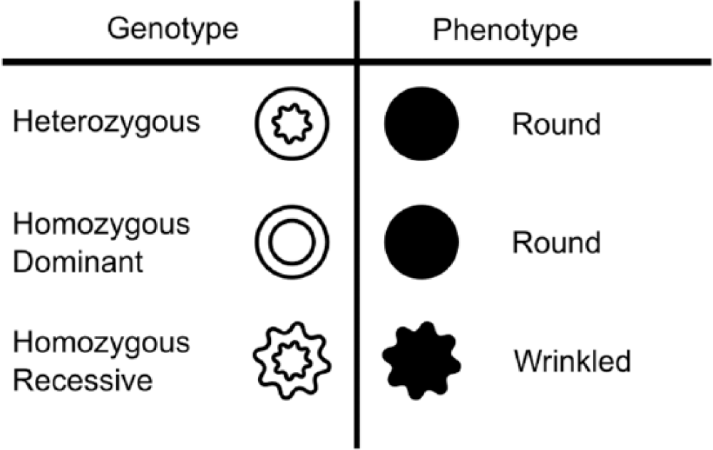
The possible genotypes and corresponding phenotypes for the garden pea’s shape trait. The gene for seed shape has two possible alleles (round and wrinkled), and the allele for round seeds is dominant. Circles denote the allele for or trait of round seeds, and stars denote the allele for or trait of wrinkled seeds. The outer shape of each icon shows the corresponding phenotype. This figure is licensed under CC BY 4.0.

Mendel theorized that there was a 50% chance of a parent passing each of its two alleles to its offspring. This theory leads to easily predictable genotypic ratios for the seed shape of offspring from two heterozygous parents (shown in Fig. 4).

Fig. 4.

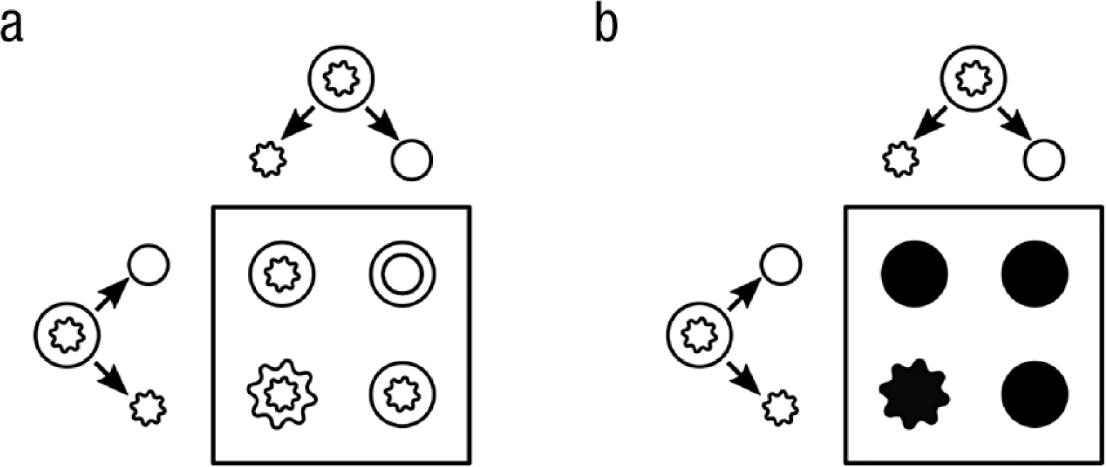
An example of Mendelian genetics with two heterozygous parents, depicted at the left and top of each square. Each parent has one allele for round seeds and one allele for wrinkled seeds, and passes along one of these alleles to each offspring. In (a), the icons inside the square denote the four genotypes that can result from the crossings of the parents’ alleles In (b), the icons inside the square denote the phenotype corresponding to each possible genotype. Circles denote the allele for the trait of round seeds, and stars denote the allele for the trait of wrinkled seeds. Although 50% of the alleles correspond to the wrinkled phenotype, only 25% of the resulting plants will have wrinkled seeds because the allele for wrinkles is recessive. This figure is licensed under CC BY 4.0.

The key to Mendel’s experiments was the ratio of phenotypes from crossings of different plants. Mendel could infer that a plant was heterozygous if it was round as a seed yet subsequently produced some wrinkled seeds. Wrinkled-seed offspring are a giveaway that the parent plant must have passed on a recessive allele, and hence must be heterozygous. As Figure 4 shows, if one crosses a heterozygous plant with itself, Mendel’s theory predicts that 75% of the seeds should be round.

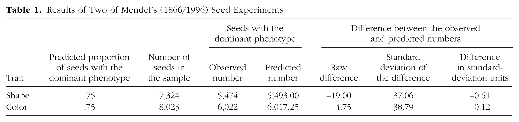
Table 1 shows Mendel’s results from crossing heterozygous plants. Of 7,324 seeds, one would expect 5,493 to be round. Mendel reported that 5,474 were round—a difference of only 19 from the number expected. Of course, the results of such experiments are variable: According to Mendel’s theory, the standard deviation of the number of round seeds in a sample of 7,324 is approximately 37 (i.e., $\sqrt{7324 \times . 75 \times . 25}$ . Thus, Mendel’s results deviated from the theoretical value by only half a standard deviation. By itself, this closeness is not enough to raise suspicion: There would be a fair chance—38%—of obtaining a closer result.

Table 1.

Results of Two of Mendel’s (1866/1996) Seed Experiments

Trait	Predicted proportion of seeds with the dominant phenotype	Number of seeds in the sample	Seeds with the dominant phenotype		Difference between the observed and predicted numbers
Trait	Predicted proportion of seeds with the dominant phenotype	Number of seeds in the sample	Observed number	Predicted number	Raw difference	Standard deviation of the difference	Difference in standard-deviation units
Shape	.75	7,324	5,474	5,493.00	−19.00	37.06	−0.51
Color	.75	8,023	6,022	6,017.25	4.75	38.79	0.12

In 1936, Fisher examined all of Mendel’s experimental outcomes. The first step was to compute each outcome’s deviation from the theoretical prediction in standard-error units. The standard error is the standard deviation of the estimated proportion and serves as a natural metric to understand how deviant observations are. Then, because Fisher was interested in the overall distance from the theoretical values, he squared every deviation and summed these values across all the experiments.

To illustrate this method, we use two experiments as examples. In the experiment on round and wrinkled seeds that we just discussed, the observed number of round seeds was 0.51 standard error below the theoretical value. In a second experiment, Mendel found that 6,022 of 8,023 seeds contained yellow, rather than green, seeds. The expected proportion was .75, or about 6,017 yellow leaves. The observed number was 5 above what was expected, a difference of a mere 0.12 standard deviation from the theoretical value (see Table 1). The theoretical value can be thought of as the bull’s-eye of a target, as shown in Figure 5a. The figure shows the standard errors as circles around the bull’s-eye. To assess how close these two experiments’ results are to the bull’s-eye, one works out the distance from the center to the point (–.51, .12), which corresponds to the number of standard errors that separate each experiment’s outcome from the theoretical value. The distance from this point to the bull’s-eye can be calculated by using the familiar Pythagorean theorem, which yields a distance of $\sqrt{. 28}$ .

Fig. 5.

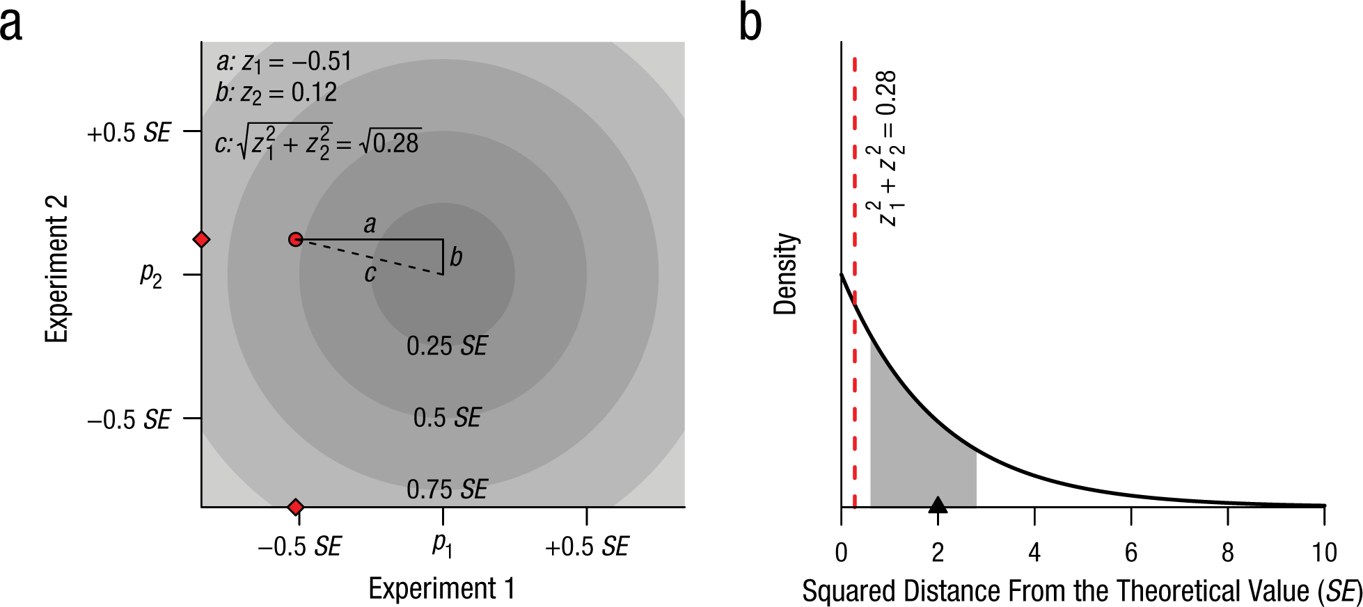
Fisher’s (1936) approach to examining whether Mendel’s results were too close to the expected values to be credible. The diagram in (a) shows how the Pythagorean theorem can be used to calculate the distance, c (in standard-error units), of the outcomes of Mendel’s seed-shape and leaf-color experiments (red circle) from the theoretical values (center of the bull’s eye, represented by p₁ and p₂). The diamonds on the axes show the individual observations in the experiments. The graph in (b) shows the distribution of the observed squared distance, assuming two experiments: a χ²(2) distribution. The expected squared distance is 2 (highlighted by the triangle on the x–axis). The probability of getting a smaller squared distance than the one observed in the two experiments in (a) is about .13, assuming Mendel’s theory is correct. The shaded region shows the middle 50% of the distribution. This figure is licensed under CC BY 4.0.

The total deviation from the theoretical value by itself does not indicate whether Mendel’s results are surprisingly close to the predictions; to determine this, Fisher (1936) compared the observed values with the sampling distribution predicted by Mendel’s theory. Sometimes the distance will be small, and other times larger, but if Mendel was right, the sum of the squared distance from the expected values along the two axes should have a χ² distribution with 2 degrees of freedom, as shown in Figure 5b. For each dimension (in this example, seed shape and seed leaf color), the outcome is expected to be somewhat off the theoretical value. The greater the number of dimensions, the greater the expected distance from the theoretical value, because each dimension contributes to the total distance. The expected squared distance for two experiments is 2. The observed squared distance for the two experiments in our example, however, is much smaller: 0.28. Specifically, the observed distance from the bull’s-eye is closer than what would be expected 87% of the time, if Mendel’s theory is correct. Although this result is far from definitive, it seems close enough to the theoretical value to cause some suspicion, because even if Mendel was right, he would rarely be expected to see observations closer. But this analysis includes only 2 of the 84 experiments reported by Mendel.

Fisher tabulated the results of all 84 of Mendel’s experiments. For clarity of presentation, in Figure 6 we have grouped the results into the 16 series suggested by Edwards (1986, Table 2, pp. 306–308).² Notice that most of the squared distances from the theoretical predictions seem to be on the low side, closer to 0 than what would be expected. Across all 84 of Mendel’s experiments, the expected average squared distance is 84. The observed squared distance is substantially less: 49.15. To illustrate how small this value is, in Figure 7 we show the χ² distribution with 84 degrees of freedom, the sampling distribution of the squared distance across all experiments assuming Mendel’s theory. The observed squared distance is so small that 99.9% of such sets of experiments would be expected to yield a larger distance. The experiments’ results are very close to the theoretical values.

Fig. 6.

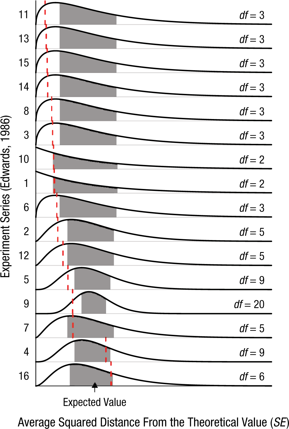
Results from Edwards’s (1986) 16 groupings of Mendel’s 84 experiments. In each of these series, the vertical dashed line indicates the observed squared distance from the theoretical value, the solid curve shows the theoretical distribution of the squared distance, and the shaded region indicates the middle 50% of the distribution. The series are ordered according to the observed deviation from the expected value and scaled by the expected value (degrees of freedom) in order for all the results to be visually aligned. This figure is licensed under CC BY 4.0.

Fig. 7.

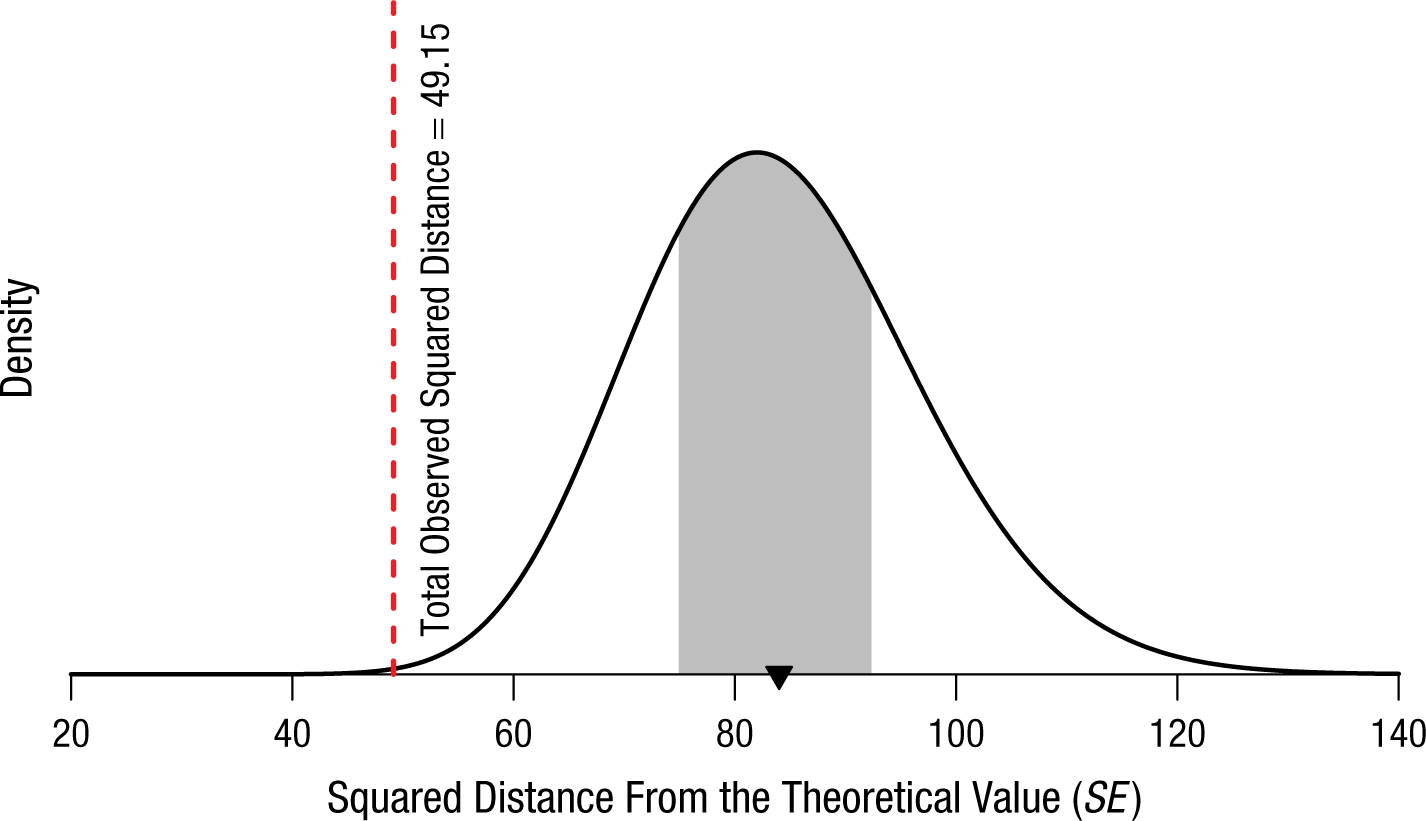
Theoretical distribution of the squared distance from the theoretical value across all 84 of Mendel’s experiments. The red line indicates the observed total squared distance of 49.15 (calculated from Edwards’s, 1986, data). There is a 99.9% chance that a random value from this distribution would be larger than 49.15. The shaded region shows the middle 50% of the distribution, and the expected value is indicated by the triangle on the x-axis. This figure is licensed under CC BY 4.0.

So what? Was Weldon (1902) right when he said that Mendel’s results were “admirably in accord with his experiment” (p. 235)? Was Pilgrim (1984) right to wonder why results that closely agreed with a theory were causing such a fuss? Or was Fisher (1936) right when he suggested that “most, if not all, of the experiments have been falsified so as to agree closely with Mendel’s expectations” (p. 132)? Do results that agree too closely with a theoretical null value actually undermine the evidence?

The last prominent statistician to weigh in on the debate was Edwards (1986), who said,

If it were just a question of having hit the bull’s eye with a single shot we might conclude . . . that Mendel was simply lucky, but when a whole succession of shots comes close to the bull’s eye we are entitled to invoke skill or some other factor. (p. 303)

Of course “skill” cannot overcome the problem of inherent random variability. Both Edwards³ and more recently Franklin (2008) suggested that Fisher’s analysis has stood the test of time: Mendel’s results are too good to be true. Yet the controversy is largely unknown outside of statistical circles. Why?

Justified suspicion that a result is tainted does not mean it is wrong: A century and a half later, we are in the lucky position of knowing that Mendel was right. Science is not always neat; biases will creep into even the most rigorous research, if only because scientific progress requires interpreting the results of experiments post hoc with incomplete information. As Dobzhansky (1967) wrote at the centennial of Mendel’s publication,

Few experimenters are lucky enough to have no mistakes or accidents happen in any of their experiments, and it is only common sense to have such failures discarded. The evident danger is ascribing to mistakes and expunging from the record perfectly authentic experimental results which do not fit one’s expectations. (p. 1588) Luckily, Mendel described his experiments in sufficient detail that they can be easily repeated. Doubt about any claim can be put to rest by rigorous replication of the procedure, provided that the theory is defined clearly enough for scientists to decide what a “replication” would be. Providing this clarity is one of the roles of a scientific paradigm.

Interpretation of results occurs in the context of scientific theory: This point seems especially obvious in the case of Mendel, given that the null value was derived from Mendel’s theory. But suppose Mendel were a fair-minded experimentalist, and one could travel back in time and confront him with Fisher’s findings? Should Mendel abandon his theory? Probably not. Although Fisher’s critique threatens the evidential force of Mendel’s experiments, Fisher (1936) himself pointed out that Mendel, or anyone else in the 19th century, could have derived genetic theory from three simple postulates (pp. 123–124); he also believed that Mendel may have done so. Fisher (1936) thought it possible that Mendel’s experiments were a “carefully planned demonstration of his conclusions” (p. 124), rather than their sole support. Mendel’s theory was strong enough to withstand Fisher’s critique of the evidence, in contrast to more recent psychological results subjected to similar scrutiny (see, e.g., Simmons & Simonsohn, 2017).

Unbelievable Null Results: LIGO and Gravity Waves

Michelson’s experiments using interferometers were not only important for their results; the Michelson interferometer is a tool that continues to be used in research. Michelson’s interferometers were about 1 m wide. Modern interferometers range from palm sized and small enough to fit in a satellite (Shepherd et al., 1993) to the immense instruments used by the LIGO project, which operates two interferometers, each with arms 4 km long.⁴

The purpose of the LIGO project is not to find evidence for the luminiferous ether; rather, the LIGO team is hunting for gravitational waves. In Einstein’s general theory of relativity, gravity is the result of changes in the geometry of space-time: A mass, such as a star, bends space-time around it. When masses accelerate in certain ways—for example, when black holes orbit one another—these distortions are supposed to cause gravitational waves that propagate away from the source.

The search for gravitational waves serves both as a test of general relativity and as new way of conducting astronomy. Scientists can use gravity waves in much the same way as they use x-rays, visible light, microwaves, and radio waves to piece together a picture of the history of the universe. Unlike light, however, gravitational waves are difficult to detect, because they involve extraordinarily subtle effects as they pass.

This is where Michelson’s interferometer plays a key role. Laser light is split, shot down two perpendicular 4-km arms, and bounced back from precisely suspended mirrors. The laser light is then recombined and passed to a detector. If the two arms are the same length, the two recombined waves cancel, and no laser light is detected. When a gravitational wave passes an interferometer, the two perpendicular arms will change in length (Fig. 8). If one arm is longer than the other, then the cancelation is imperfect, and some of the light will make it to the detector. Space-time distortion from a passing gravitational wave shows up as fluctuations in the amount of laser light at the detector.

Fig. 8.

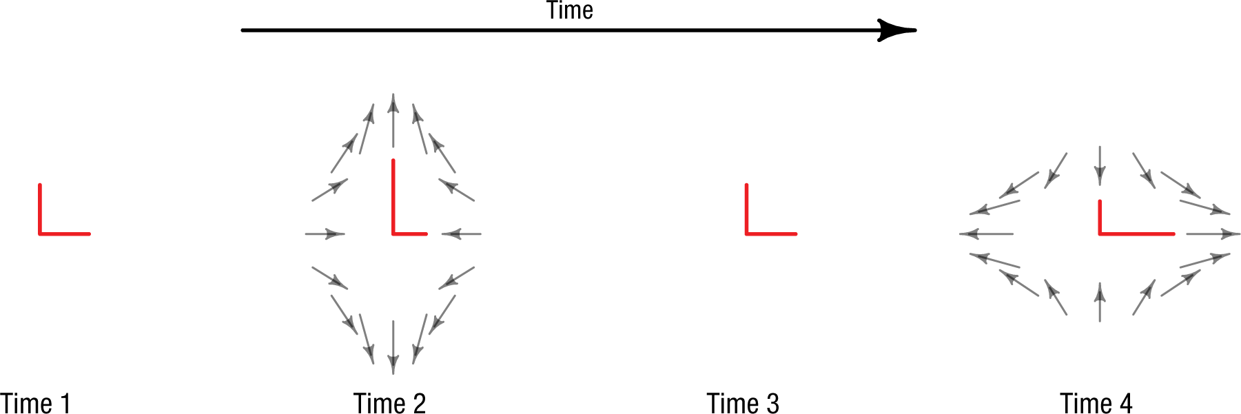
How gravitational waves distort the length of the two perpendicular arms of the Michelson interferometers operated by the Laser Interferometer Gravitational-Wave Observatory. Before the gravity wave passes (Time 1), the two arms of the interferometer are the same length. The gravity wave distorts space-time around the interferometer, lengthening one path and shortening the other (Time 2); the paths then return to their original lengths (Time 3), and the opposite lengthening and shortening occurs (Time 4). This figure is licensed under CC BY 4.0.

Because fluctuations can happen for reasons other than gravitational waves, the LIGO team uses multiple sites—one in Washington and one in Louisiana—to cross-check its results. The team also cooperates with the team operating the smaller, 3-km Virgo interferometer in Italy (Fig. 9). The LIGO team looks for “unusual” events that occur in multiple detectors. Looking for correlations across these sites allows noisy fluctuations in only one detector to be discounted.

Fig. 9.

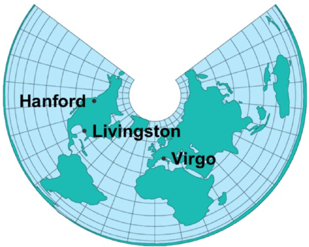
Locations of the Laser Interferometer Gravitational-Wave Observatory (LIGO) interferometers in the United States (Hanford, Washington, and Livingston, Louisiana) and the Virgo interferometer in Italy (near Pisa). This figure is licensed under CC BY 4.0.

LIGO’s first attempt at detecting gravitational waves in 2002 yielded a null result; that is, the data were deemed consistent with background noise (LIGO Scientific Collaboration, 2004). This was expected, though, because the detectors were not yet at full sensitivity. The introduction to the report on this run is worth quoting directly:

The first detection of gravitational wave bursts requires stable, well understood detectors, well-tested and robust data processing procedures, and clearly defined criteria for establishing confidence that no signal is of terrestrial origin. None of these elements were firmly in place as we began this first LIGO science run; rather, this run provided the opportunity for us to understand our detectors better, exercise and hone our data processing procedures, and build confidence in our ability to establish the detection of gravitational wave bursts in future science runs. Therefore, the goal for this analysis is to produce an upper limit on the rate for gravitational wave bursts, even if a purely statistical procedure suggests the presence of a signal above background. (LIGO Scientific Collaboration, 2004, pp. 102001–102003)

Unlike Michelson at the conclusion of his 1881 experiment, the LIGO team was unwilling to accept the null hypothesis on the basis of a noisy experiment; as did Michelson and Morley in 1887, the LIGO team stated their results in terms of placing an upper limit on a quantity of interest.⁵

From the first failure followed more. Six additional runs over more than a decade yielded no evidence—at least none the team was willing to accept as inconsistent with background noise—of gravitational waves. LIGO became “advanced LIGO” as the team improved the sensitivity of their instruments. With each failure using a more sensitive device, a new upper limit was established. The titles of the reports tell the story: “Upper Limits on Gravitational Wave Bursts in LIGO’s Second Science Run” (LIGO Scientific Collaboration, 2005), “Upper Limits on Gravitational Wave Emission From 78 Radio Pulsars” (LIGO Scientific Collaboration, 2007), and “Improved Upper Limits on the Stochastic Gravitational-Wave Background from 2009-2010 LIGO and Virgo Data” (LIGO and Virgo Collaboration, 2014). From 2004 through 2016, this work spawned about 100 publications that characterized the instruments, algorithms, and their improvements or presented data from science runs.

Finally, in 2016, the team published a report announcing the detection of gravitational waves from the merger of two black holes (LIGO Scientific Collaboration and Virgo Collaboration, 2016). But what happened in the years before this detection is of greater interest for present purposes. Why were the LIGO team unwilling to accept the null results and hence the possibility that there were no gravitational waves? What was the difference between Michelson and Morley’s situation in the late 19th century and the LIGO team’s situation in the early 21st? We believe there were several differences:

The prospect of more sensitive experiments: The LIGO team was constantly improving their instruments and knew that more sensitive tests were just around the corner.

Strong theoretical expectations and low sensitivity: The LIGO team knew early on that their instruments were not sensitive enough to detect many gravitational-wave events of interest, should they exist. Unlike Michelson and Morley’s null result, the LIGO team’s null results were not unexpected from the theory.

No theoretical rival: Einstein’s general theory of relativity has withstood numerous tests over the past century. There is no rival to the theory that could take its place should gravitational waves not exist. Plunging a field into crisis is not something to be taken lightly, particularly at the expense of such a well-established theory.

These three conditions made the acceptance of the null hypothesis difficult, even on the basis of multiple “failed” LIGO runs. Luckily, the persistence paid off. Since the 2016 detection, the team has made several new detections. The ability to consistently detect and characterize gravitational waves has the potential to usher in a new era of gravitational-wave astronomy, which would not have happened if the team had accepted the null hypothesis and given up.

Conclusion

In each of these three examples, a type of statistical null was rejected or accepted in accordance with pragmatic considerations of what would facilitate the accumulation of scientific knowledge. Michelson and Morley’s null result, for instance, appeared compelling because an alternative to wave theory could account for it. On the other hand, there is no alternative to the theory of general relativity, so accepting the null hypothesis that there are no gravitational waves would throw physics into crisis, and indeed the LIGO team did not accept the null hypothesis. Fisher noted that Mendel could have derived his predictions from three simpler theoretical postulates, rather than from the data themselves. The evidential force of Mendel’s too-small deviations from theoretical predictions was considered in a broader scientific context. In all three cases, the evidential value of the data was considered along with higher-level theoretical concerns within a theoretical paradigm. The experiments were not meant to show an isolated effect, or lack thereof; rather, they were tests or demonstrations of aspects of a broad theory.

In contrast, paradigmatic research programs—with concordant null hypotheses—have become scarce in the contemporary field of psychology. The paradigmatic progress exemplified by these three examples would not be possible within psychology’s current research landscape, which closely aligns with the Kuhnian description of a preparadigm science. This was not always true; in the mid 20th century, psychological theorizing had coalesced into several broad paradigmatic perspectives (e.g., cognitive dissonance theory—Festinger, 1957). However, the subsequent decades saw psychology transform back into a discipline more clearly characterized by a preparadigm population of microtheories. Often, these microtheories have consisted solely of the described effect, followed by the word theory or model, and thus have been empty restatements. Insofar as they can be construed as unfalsifiable, one might call them pseudotheories (Fiedler, 2004). To the extent that these descriptive theories are arrived at entirely post hoc, they can constitute entire pseudoscience disciplines (Lakatos, 1970).

Consider the facial feedback hypothesis (Strack, Martin, & Stepper, 1988), according to which feedback from the face modulates emotion. Wagenmakers et al. (2016) recently attempted to replicate the original study, obtaining a null result across several labs and thousands of participants. In normal science, this might lead to a paradigmatic crisis or new boundary conditions, either of which could be construed as progress. Instead, Wagenmakers et al. simply claimed a failure to replicate the original result, leaving Strack (2016) to offer a series of post hoc reasons why it might not have been replicated. It is not clear what was learned from the episode, because the facial feedback hypothesis is not strongly linked to a broader paradigm positing boundary conditions and mechanisms; it is a label for an effect. When an effect stands on its own, rather than in relation to a paradigm, the implications a null result has for the progress of psychological science are unclear.⁶

On the surface, psychology espouses the same standards of hypothesis testing as most mature sciences: a Popperian (1935/2002) emphasis on falsificationism predicated on hypotheses derived from explanatory paradigms. These hypotheses typically constitute clear predictions that distinguish the underlying explanatory accounts of distinct paradigms, allowing for the specification and testing of theoretical boundary conditions that illuminate the cases in which a particular paradigm may be more or less explanatory compared with its rivals (McGuire, 2013). Within the context of current psychology, theoretical boundary conditions necessarily take on a different character, given that “theories” are often little more than descriptions of phenomena, with “boundaries” that cannot extend beyond descriptions of individual effects.

When falsification can no longer be tethered to the boundary conditions of explanatory paradigms, Popperian null-hypothesis testing shifts to testing the reliability of individual effects; if an effect is not replicated as predicted, it has been “falsified” (Ferguson & Heene, 2012). Accordingly, the historical emphasis on theory-framed hypothesis testing has been replaced by an emphasis on the statistical significance of hypothesized effects (e.g., Benjamin et al., 2018; Open Science Collaboration, 2012, 2015; Simmons, Nelson, & Simonsohn, 2011), and these predictions are increasingly tested against a preregistered hypothesis derived from previous outcomes. In a normal-science setting, experimental hypotheses follow from predictions that themselves follow from well-developed theories, so there is no need for preregistering the hypotheses. Moreover, replacing paradigmatic falsifiability with replicability of effects discourages researchers from attending to the paradigmatic principles that allow for contextualized assessments of the evidential value of a given replication “failure” (Stroebe & Strack, 2014). This further entrenches, rather than opposes, the preparadigm nature of much of psychological science today (also see Fiedler, Kutzner, & Krueger, 2012).

Acting within normal science, all the experimenters we have highlighted—Michelson and Morley, Mendel, and the LIGO team—are celebrated for their careful experimentation. Michelson invented multiple iterations of his device to reduce the noise in his measurements. Mendel grew thousands of pea plants across 84 experiments to demonstrate his theory. The LIGO team invested a decade honing their experimental skills before finding a single gravitational wave. This attention to detail is possible when scientific progress is not defined by arguments over individual effects and statistical significance, but rather is guided by work within, or opposing, a broad paradigm. Only if psychology reasserts itself as a normal science will it become a field unified by wide-ranging theoretical perspectives and a field in which evidence for statistical regularities is valued at least as much as significant differences.

Supplementary Material

Open Practices Disclosure, MoreyAMPPSOpenPracticesDisclosure-v1-0 – Beyond Statistics: Accepting the Null Hypothesis in Mature Sciences

Open Practices Disclosure, MoreyAMPPSOpenPracticesDisclosure-v1-0 for Beyond Statistics: Accepting the Null Hypothesis in Mature Sciences by Richard D. Morey, Saskia Homer, and Travis Proulx in Advances in Methods and Practices in Psychological Science

Footnotes

Action Editor

Daniel J. Simons served as action editor for this article.

Author Contributions

The main concept of this article is due to R. D. Morey, as are the two physics examples; S. Homer contributed the majority of the genetics examples. Both R. D. Morey and S. Homer developed the commentary on these examples. T. Proulx contributed the philosophy-of-science elements.

ORCID iD

Saskia Homer

Declaration of Conflicting Interests

The author(s) declared that there were no conflicts of interest with respect to the authorship or the publication of this article.

Open Practices

All data and materials, including the code for generating the analyses and figures and data from Michelson and Morley (1887) and Mendel (1866/1996), have been made publicly available via GitHub and can be accessed at https://github.com/richarddmorey/nullHistoryAMPPS. The complete Open Practices Disclosure for this article can be found at http://journals.sagepub.com/doi/suppl/10.1177/2515245918776023. This article has received badges for Open Data and Open Materials. More information about the Open Practices badges can be found at .

Notes

References

Benjamin

D. J.

Berger

Johannesson

Nosek

B. A.

Wagenmakers

E.-J.

Berk

. . . Johnson

(2018). Redefine statistical significance. Nature Human Behaviour, 2, 6–10.

Dobzhansky

(1967). Looking back at Mendel’s discovery. Science, 156, 1588–1589.

Edwards

A. W. F.

(1986). Are Mendel’s results really too close? Biological Reviews, 61, 295–312.

Einstein

(2013). On the electrodynamics of moving bodies ( Saha

Trans.). Retrieved from https://en.wikisource.org/wiki/On_the_Electrodynamics_of_Moving_Bodies_(1920_edition) (Original work published 1905)

Eisele

Nevsky

A. Y.

Schiller

(2009). Laboratory test of the isotropy of light propagation at the 10⁻¹⁷ level. Physical Review Letters, 103, Article 090401. doi:10.1103/PhysRevLett.103.090401

Ferguson

C. J.

Heene

(2012). A vast graveyard of undead theories: Publication bias and psychological science’s aversion to the null. Perspectives on Psychological Science, 7, 555–561. doi:10.1177/1745691612459059

Festinger

(1957). A theory of cognitive dissonance. Stanford, CA: Stanford University Press.

Feynman

R. P.

(1985). QED: The strange theory of light and matter. Princeton, NJ: Princeton University Press.

Fiedler

(2004). Tools, toys, truisms, and theories: Some thoughts on the creative cycle of theory formation. Personality and Social Psychology Review, 8, 123–131. doi:10.1207/s15327957pspr0802_5

10.

Fiedler

Kutzner

Krueger

J. I.

(2012). The long way from α-error control to validity proper: Problems with a short-sighted false-positive debate. Perspectives on Psychological Science, 7, 661–669. doi:10.1177/1745691612462587

11.

Fisher

R. A.

(1936). Has Mendel’s work been rediscovered? Annals of Science, 1, 115–137. doi:10.1080/00033793600200111

12.

Franklin

(2008). The Mendel-Fisher controversy: An overview. In Franklin

Edwards

A. W. F.

Fairbanks

D. J.

Hartl

D. L.

Seidenfeld

(Eds.), Ending the Mendel-Fisher controversy (pp. 1–77). Pittsburgh, PA: University of Pittsburgh Press.

13.

Gigerenzer

Krauss

Vitouch

(2004). The null ritual: What you always wanted to know about significance testing but were afraid to ask. In Kaplan

(Ed.), The Sage handbook of quantitative methodology for the social sciences (pp. 391–408). Thousand Oaks, CA: Sage.

14.

Kuhn

T. S.

(1962). The structure of scientific revolutions. Chicago, IL: University of Chicago Press.

15.

Lakatos

(1970). History of science and its rational reconstructions. In Proceedings of the biennial meeting of the Philosophy of Science Association, 1970, 91–136.

16.

LIGO and Virgo Collaboration. (2014). Improved upper limits on the stochastic gravitational-wave background from 2009-2010 LIGO and Virgo data. Physical Review Letters, 113, Article 231101. doi:10.1103/PhysRevLett.113.231101

17.

LIGO Scientific Collaboration. (2004). First upper limits from LIGO on gravitational wave bursts. Physical Review D, 69, Article 102001. doi:10.1103/PhysRevD.69.102001

18.

LIGO Scientific Collaboration. (2005). Upper limits on gravitational wave bursts in LIGO’s second science run. Physical Review D, 72, Article 062001. doi:10.1103/PhysRevD.72.062001

19.

LIGO Scientific Collaboration. (2007). Upper limits on gravitational wave emission from 78 radio pulsars. Physical Review D, 76, Article 042001. doi:10.1103/PhysRevD.76.042001

20.

LIGO Scientific Collaboration and Virgo Collaboration. (2016). Observation of gravitational waves from a binary black hole merger. Physical Review Letters, 116, Article 061102. doi:10.1103/PhysRevLett.116.061102

21.

McGuire

W. J.

(2013). An additional future for psychological science. Perspectives on Psychological Science, 8, 414–423. doi:10.1177/1745691613491270

22.

Meehl

P. E.

(1978). Theoretical risks and tabular asterisks: Sir Karl, Sir Ronald, and the slow progress of soft psychology. Journal of Consulting and Clinical Psychology, 46, 806–834.

23.

Mendel

(1996). Experiments in plant hybridization ( Bateson

Trans.). Retrieved from http://www.esp.org/foundations/genetics/classical/gm-65.pdf (Original work published 1866)

24.

Michelson

A. A.

(1881). The relative motion of the Earth and the luminiferous ether. American Journal of Science, 22, 120–129.

25.

Michelson

A. A.

Morley

E. W.

(1887). On the relative motion of the Earth and the luminiferous ether. American Journal of Science, 34, 333–345.

26.

Open Science Collaboration. (2012). An open, large-scale, collaborative effort to estimate the reproducibility of psychological science. Perspectives on Psychological Science, 7, 652–655.

27.

Open Science Collaboration. (2015). Estimating the reproducibility of psychological science. Science, 349, Article aac4716. doi:10.1126/science.aac4716

28.

Piegorsch

W. W.

(1990). Fisher’s contributions to genetics and heredity, with special emphasis on the Gregor Mendel controversy. Biometrics, 46, 915–924.

29.

Pilgrim

(1984). The too-good-to-be-true paradox and Gregor Mendel. Journal of Heredity, 75, 501–502.

30.

Popper

(2002). Logic of scientific discovery. London, England: Routledge Classics. (Original work published 1935)

31.

Ritz

(1980). Critical researches on general electrodynamics ( Lucier

Trans.). Retrieved from Mitchell Memorial Library, Mississippi State University, Mississippi State, MS. (Original work published 1908)

32.

Shepherd

G. G.

Thuillier

Gault

W. A.

Solheim

B. H.

Hersom

Alunni

J. M.

. . . Wimperis

(1993). WINDII, the wind imaging interferometer on the Upper Atmo-sphere Research Satellite. Journal of Geophysical Re-search: Atmospheres, 98, 10725–10750. doi:10.1029/93JD00227

33.

Simmons

J. P.

Nelson

L. D.

Simonsohn

(2011). False-positive psychology: Undisclosed flexibility in data collection and analysis allows presenting anything as significant. Psychological Science, 22, 1359–1366. doi:10.1177/0956797611417632

34.

Simmons

J. P.

Simonsohn

(2017). Power posing: P-curving the evidence. Psychological Science, 28, 687–693. doi:10.1177/0956797616658563

35.

Sterling

T. D.

Rosenbaum

W. L.

Weinkam

J. J.

(1995). Publication decisions revisited: The effect of the outcome of statistical tests on the decision to publish and vice versa. The American Statistician, 49, 108–112. doi:10.1080/00031305.1995.10476125

36.

Strack

(2016). Reflection on the smiling Registered Replication Report. Perspectives on Psychological Science, 11, 929–930. doi:10.1177/1745691616674460

37.

Strack

Martin

L. L.

Stepper

(1988). Inhibiting and facilitating conditions of the human smile: A nonobtrusive test of the facial feedback hypothesis. Journal of Personality and Social Psychology, 54, 768–777.

38.

Stroebe

Strack

(2014). The alleged crisis and the illusion of exact replication. Perspectives on Psychological Science, 9, 59–71. doi:10.1177/1745691613514450

39.

Wagenmakers

E.-J.

Beek

Dijkhoff

Gronau

Q. F.

Acosta

Adams

R. B.

Jr. . . . Zwaan

R. A.

(2016). Registered Replication Report: Strack, Martin, & Stepper (1988). Perspectives on Psychological Science, 11, 917–928. doi:10.1177/1745691616674458

40.

Weldon

W. F. R.

(1902). Mendel’s laws of alternative inheritance in peas. Biometrika, 1, 228–254.

Supplementary Material

Please find the following supplemental material available below.

For Open Access articles published under a Creative Commons License, all supplemental material carries the same license as the article it is associated with.

For non-Open Access articles published, all supplemental material carries a non-exclusive license, and permission requests for re-use of supplemental material or any part of supplemental material shall be sent directly to the copyright owner as specified in the copyright notice associated with the article.

0.00 MB

0.29 MB