Sage Journals: Discover world-class research

Abstract

The recent field-wide emphasis on power has brought the number of participants used in psychological experiments into focus. Social psychology typically follows a tradition in which many participants perform a small number of trials each; in psychophysics, the tradition is to include only a few participants, who perform many trials each; and the tradition in cognitive psychology falls in between, balancing the number of participants and trials. We ask whether it is better to add trials or to add participants if one wishes to increase power. The answer is straightforward—greatest power is achieved by using more people, and the gain from adding people is greater than the gain from adding trials. In light of these results, the design parameters in the social psychology tradition seem ideal. Yet there are conditions in which one may trade people for trials with only a minor decrement in power. Under these conditions, the limiting factor is the trial-to-trial variability rather than the variability across people in the population. These conditions are highly plausible, and we present a theoretical argument as to why. We think that most cognitive effects are characterized by stochastic dominance; that is, everyone’s true effect is in the same direction. For example, it is plausible that when performing the Stroop task, all people truly identify congruent colors faster than incongruent ones. When dominance holds, small mean effects imply a small degree of variability across the population. It is this degree of homogeneity, the consequence of dominance, that licenses the design parameters of the cognitive psychology and psychophysics traditions.

Keywords

power within-participants designs open materials

The practice of psychological science is going through a period of rapid transition during which methodological concerns are front and center. One long-standing, salient concern is that too many experiments are underpowered (Cohen, 1962; Maxwell, 2004; Szucs & Ioannidis, 2017). There are two consequences of underpowered designs. First, if a design is underpowered, then there is an increased chance of failing to detect an effect. When this failure happens, the interpretation of the results is muddied, as it is unclear if the failure reflects a lack of power or a truly null effect. Second, and perhaps more perniciously, the prevalence of underpowered studies as a whole is taken as a signal that the literature is not trustworthy. Indeed, it is an indicator that researchers may be massaging variability to produce significance (Button et al., 2013; Gelman & Loken, 2014; Ioannidis, 2005).

One solution to the problem of underpowered designs is simply to add more participants. As Baumeister (2016) noted, typical sample sizes have risen over the decades from 10 to 20 to 50, and now to more. Indeed, if one takes power seriously, then experiments for typically small effects should have several hundred observations. Table 1 provides the minimum sample sizes per group needed for .80 power to detect small, moderate, and large effects (Cohen, 1988) with independent- and paired-samples t tests, given a .05 α level. Should experimental psychologists be running hundreds of participants in every experiment?

Table 1.

Minimum Sample Sizes per Group for Independent- and Paired-Samples t Tests to Detect Small, Medium, and Large Effects

	Effect size
Design	Small (d = 0.2)	Medium (d = 0.5)	Large (d = 0.8)
Two independent samples	394	64	26
Paired samples	199	34	15

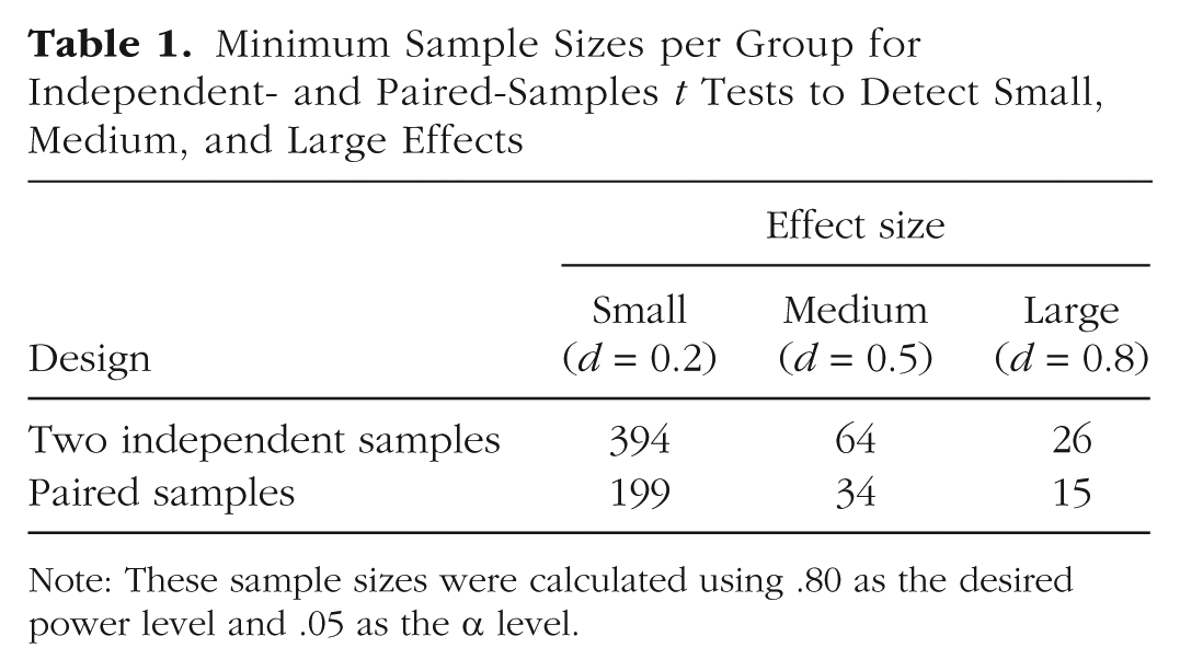
Note: These sample sizes were calculated using .80 as the desired power level and .05 as the α level.

One of the most fruitful traditions in psychology is the psychophysics tradition. Consider, for example, Blakemore and Campbell’s (1969) classic adaptation experiment that first showed orientation- and frequency-selective neural responses. There were only 2 participants, C. B. and F. W. C., who maybe not so surprisingly have the same initials as the authors. Logan and Cowan’s (1984) classic stop-process article, the one that launched a subfield of action control, had only 3 participants (including G. L.). The first author of the current article has twice published reports on experiments with only 3 people (Ratcliff & Rouder, 1998; Rouder, Morey, Cowan, & Pfaltz, 2004).

The typical experimental design in the psychophysics tradition may be described by three properties: (a) the use of very small numbers of participants, (b) the use of within-participants manipulations, and (c) the use of very large numbers of trials per participant. This tradition may be compared with two others. Experiments in the cognitive tradition usually include moderate numbers of participants (e.g., 20), use both within-participants and between-participants manipulations but more typically the former, and include moderate numbers of trials per participant (e.g., 10–100). In the social psychology tradition, experiments include a great many participants, often use between-participants groupings, and have a handful of observations per participant.

In this article, we explore these traditions’ overall power to detect effects in within-participants designs. Suppose, for example, that one wishes to partition 2,000 observations across two conditions. The psychophysics-design option might be to run 2 participants for 1,000 trials each, dividing those 1,000 trials evenly between the two conditions. The cognitive-design option might be to run 20 participants with 50 observations in each of the two conditions. The social psychology–design option might be to run 1,000 people, each of whom completes a single trial in each condition. In the formal analysis that follows, we seek the option that has the highest power to detect an effect across the two conditions at a fixed level of Type I error. There are other criteria for assessing the usefulness of design options, of course, but the criterion of highest power seems like a good start.

Disclosures

The integrated LaTeX and R code that produced the authors’ version of this article has been made publicly available at GitHub (https://github.com/PerceptionAndCognitionLab/stat-sampsize). This code typesets the text and equations, performs the evaluation and simulation of power, and draws the figures.

Which Design Tradition Leads to the Highest Power?

Our approach to evaluating the trade-off between the number of trials per participant and the number of participants is as follows: We suppose that participants provide continuously valued observations in two conditions, generically called the treatment and control conditions. An example might be a priming experiment in which primed and unprimed stimuli are presented in the treatment and control conditions, respectively. We assume that each of I participants provides K observations in each condition. Our goal is to compute power as a function of I, the number of participants, and K, the number of observations per participant per condition.

The derivation is a bit long and provided in the appendix at the end of this article. The key expression for computing power is the noncentrality parameter of the test. In brief, this parameter describes where the t is centered. The greater the value of the noncentrality parameter, the larger the expected t values and the greater the power. So, by studying the expression for noncentrality, we can gain insight into whether it is better to increase the number of participants or the number of trials per participant.

The noncentrality parameter, denoted λ, is defined as follows:

λ = \sqrt{μ^{2} \times \frac{I K}{K σ_{β}^{2} + 2 σ^{2}}} .

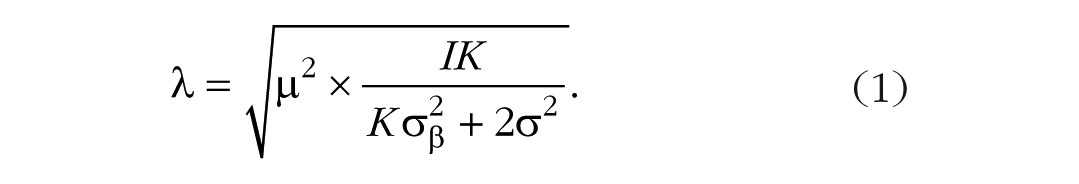
The value of the noncentrality parameter depends on three quantities besides I and K. One is µ, which is the size of the effect. It is a population mean—the true average effect across all individuals in the population. There are also two variabilities represented in Equation 1: σ² is the variability for replicates, that is, for different observations from a given person within one of the conditions; $σ_{β}^{2}$ is the variability of the true effect across people. These quantities are defined formally in the appendix.

From Equation 1, we reach a preliminary answer to the question of whether adding more people or adding more trials better powers experiments. The equation shows that increasing the number of people, I, always results in greater power than increasing the number of replicates, K, because although both I and K enter into the numerator, K also enters into the denominator. Hence, noncentrality must increase at a greater rate with I than with K. Adding more people results in a more powerful design than adding more trials. The design parameters in the social psychology tradition are best from a power perspective.

Unfortunately, these design parameters are not as appealing as those in the cognitive psychology and psychophysics tradition. The reason is the cost in money and time of running the experiment. The marginal cost of adding more trials—say, asking each participant to stay an additional few minutes—is often far less than the marginal cost of recruiting more participants. Before adopting the social psychology trade-off, it is wise to understand how much power is gained with that approach.

We show here that for some cases, the gain in power from adding participants rather than adding trials is marginal. Our approach is to pick reasonable values for the inputs in Equation 1 and examine how power changes as the numbers of people and trials are varied. Consider a typical priming effect with primed and unprimed (control) stimuli. The dependent measure is response time (RT), and, overall, responses are relatively accurate and fast (e.g., RT < 1 s). In tasks that are performed quickly and accurately, there is often a fair amount of variation across trials, and it is not uncommon to see responses as fast as 250 ms and as slow as 1,500 ms. In this case, 300 is a reasonable value of σ, the variability across repeated trials for the same participant in the same condition. Priming effects can be quite subtle, and means are on the order of 40 ms, so we use that value for µ. The remaining setting is for σ_β, which denotes how variable the effect is across people. Consider the case in which σ_β is 28 ms, which is reasonable for a 40-ms effect.

The trade-off for this case is shown in Figure 1a. Power to detect this 40-ms effect is plotted as a function of the number of trials per condition (K), separately for each of four different numbers of participants (I). The critical question is about what happens when I is traded for K. The plotted points show power for the values of I and K that result in a total of 1,000 observations (i.e., I × K = 1,000). These points form an iso-sample-size power curve, and they show that it is better to have large numbers of people and smaller numbers of trials per participant. The size of this effect is relatively minor in Figure 1a; I and K trade off fairly well. If recruiting additional people is resource expensive, then in this case, it makes sense to forgo these additional people and instead run additional trials.

Fig. 1.

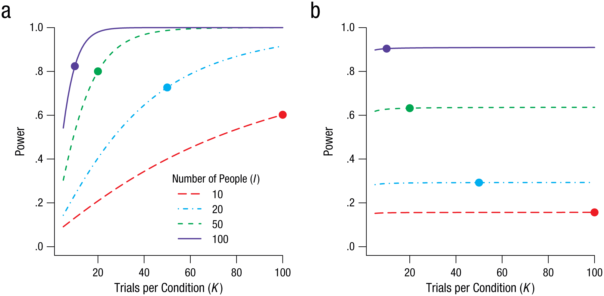
Illustration of how power changes as a function of I, the number of participants, and K, the number of observations per condition per participant. The graph in (a) shows the trade-off between these two design parameters when population variability (σ_β = 28 ms) is small relative to trial variability (σ = 300 ms). The graph in (b) shows the trade-off when population variability (σ_β = 3) is large relative to trial variability (σ = 1). The plotted point on each curve indicates the values of I and K that provide 1,000 observations.

Yet there are cases in which the power achieved using design parameters typical in the social psychology tradition is dramatically better than the power achieved with the design parameters typical in the cognitive psychology and psychophysics traditions. In these cases, researchers cannot overcome the limitations of testing a small number of people by using large numbers of trials. Consider a preference-ratings task used to assess whether caffeine in soft drinks serves as a flavor enhancer. We take decaffeinated Coke as a standard, and to make a well-controlled caffeinated version, we add anhydrous caffeine in sufficient amounts to make the flavor noticeably more bitter. Then we ask people to judge how well they like a series of samples, some of which are the decaffeinated Coke and others of which are the caffeinated Coke. The dependent variable is a Likert rating on a 5-point scale, and we assume that repeated ratings for the same person and same beverage have a relatively small variability, say, a standard deviation of 1 point on the Likert scale (σ = 1). We also assume that, overall, people prefer the sweeter Coke, and the decaffeinated version receives an average rating that is 1 point higher than the caffeinated version (µ = 1). Finally, and critically, we assume that tastes vary; some people prefer the sweetness of the decaffeinated version, others do not have a preference, and still some others prefer the more bitter, caffeinated version. Therefore, the range of effects of adding the anhydrous caffeine may be large, and we set $σ_{β}^{2}$ to 3. Figure 1b captures this case, and as it shows, trading people for trials will not be a useful strategy. Even with large numbers of trials, one must use a large number of people to gain sufficient power.

The key quantity for determining whether people can safely be traded for trials is the variability of the effect in the population, $σ_{β}^{2}$ , relative to the trial-by-trial variability, σ². When this ratio is small, as it is for the priming example, people may be traded safely for trials. When this ratio is large, however, as it is for the beverage-preference example, lowering the number of people results in degraded power.

The Dominance Constraint in Action

Our discussion thus far shows the appeal of the design tradition in social psychology, in which there are many participants per experiment. Adding observations by adding people, rather than trials, results in better accounting of variability across people. We suspect that this dynamic may not be known to many cognitive psychologists.

Fortunately, the loss in power for the design parameters in the cognitive psychology and psychophysics traditions is marginal when there is little variability in the effect across people relative to the trial-by-trial variability. Given the appeal of these traditions when it comes to cost, when designing an experiment, it is helpful to know whether people can be safely traded for trials, that is, whether the variability of the effect in the population is small relative to the trial-by-trial variability. In the remainder of this article, we provide a theoretical argument why we think this is very often the case.

Dominance defined

We start by noting that for most effects, there is an anticipated, or positive, direction. For example, we would expect more intense startle responses the stronger the stimuli used to provoke them. In fact, perhaps there are no individuals who respond with more intensity to weaker than to stronger startle stimuli. We use the term dominance to refer to this condition in which the ordering of responses is the same for all people. In the case of startle responses, for every person, the distribution of responses for stronger stimuli dominates that for weaker stimuli.

This dominance constraint may well be a hallmark of many tasks. For example, we suspect that dominance holds when stimuli differ in strength, say, in perception and memory tasks. We also suspect that it holds in priming and context tasks. Take, for example, the Stroop task. It is plausible that all individuals truly respond more quickly to congruent than to incongruent items, and that no individual truly responds quicker to incongruent than to congruent items.

Let β_i denote the true effect of the ith individual. Dominance means that β_i, is positive for all people. In the Stroop task, for example, if β_i is greater than 0, we say that the ith person identifies incongruent colors truly more slowly than congruent ones. Note that dominance applies to true values rather than to sample values. True values are latent, but they would be observed with unlimited numbers of trials. We may observe a few sample effects that are negative because of noise, but if dominance holds, sample effects tend to be positive more often than negative. Once sample noise is modeled, the resulting latent true values are all positive.

Dominance and power

Our main theoretical result is that if dominance holds, then the experimenter can trade people for trials while maintaining power. Figure 2 shows how. In Figure 2a, two possible (candidate) distributions for β are shown. One is a normal distribution with a mean of 40 ms and a standard deviation of 30 ms. Although normal distributions are popular in linear models, they imply indominance. In the case of the Stroop task, for example, this distribution would indicate that for many people, β_i is greater than 0; they obey the usual constraint, responding more slowly to incongruent stimuli than to congruent ones. But for other people, a minority for sure, the ordering is the opposite! These people are Stroop anomalous in the sense that they truly respond quicker to incongruent than to congruent items.

Fig. 2.

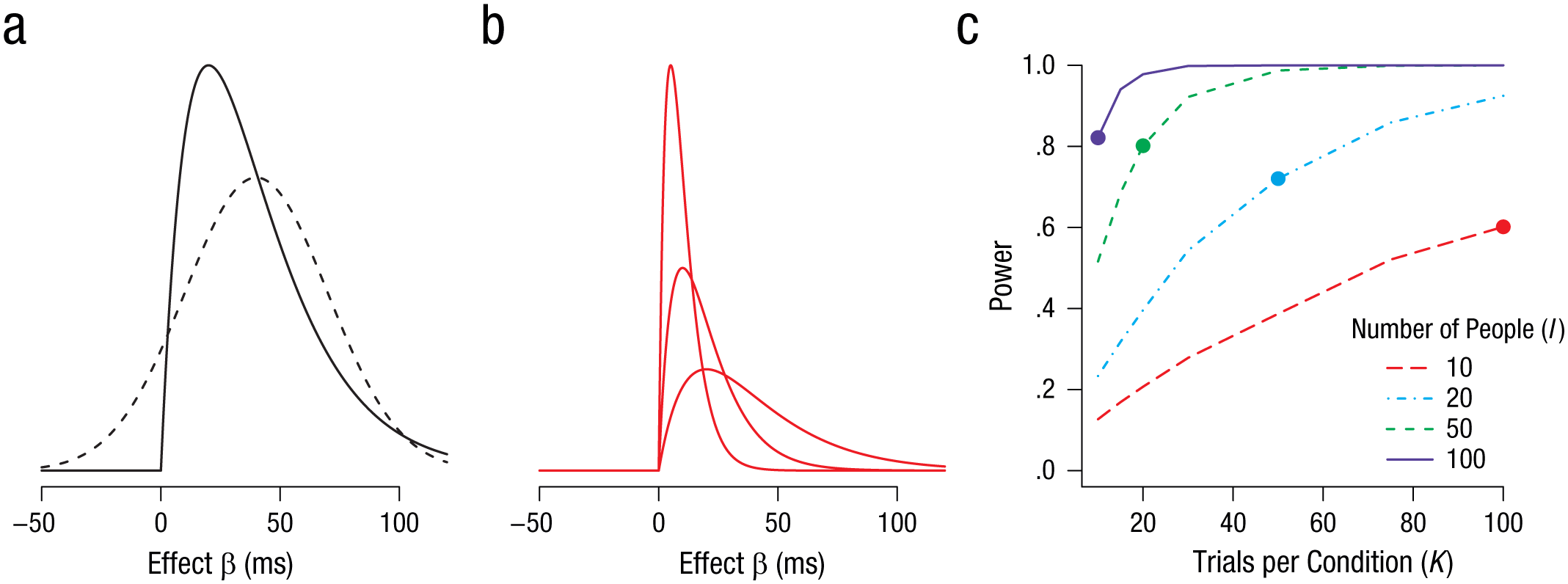
Stochastic dominance and power. The graph in (a) shows two possible distributions for true individual effects. The normal distribution (dashed line) indicates indominance, as its range includes both positive and negative effects. The skewed distribution (solid line) indicates dominance because there are no individuals with true negative effects. In some skewed distributions, the mean and standard deviation are proportional, so small means correspond to small standard deviations. This is the case, for example, for the gamma distributions shown in (b). The graph in (c) illustrates power as a function of trials per condition (K), given the skewed distribution in (a), separately for each of four numbers of participants (I). The plotted point on each curve indicates the values of I and K that provide 1,000 observations. In this dominance situation, researchers may trade people for trials.

Figure 2a also shows an alternative distribution that we find far more reasonable for many tasks. This skewed distribution for β_i is constrained to be positive for all people. One of the key differences between the two distributions in Figure 2a is the relationship between mean and variance. With normal distributions, there is no relationship. The variability and the mean are both statistically and conceptually independent. This independence does not hold for the skewed distributions shown in Figure 2b. In these cases, the mean and the variability are positively related. As the effect becomes smaller, not only does the mean decrease, but so too does the variability. The dominance constraint implies that it is impossible to have small effects with big variances. Most effects in psychological sciences are relatively small compared with the trial-by-trial variability. The dominance principle implies that the variation across people is relatively small as well. And in that case, researchers may be able to trade people for trials. Figure 2c shows the corresponding power for the skewed distribution in Figure 2a as a function of the number of trials, for four different sample sizes. The values shown come from simulations of 10,000 iterations per combination of number of participants and number of trials per condition. The graph shows that trading people for trials results in just a marginal reduction of power.

Indominance

Dominance need not always hold, of course. There may be tasks in which some people engage in a different strategy than others, or in which some people have different sets of preferences than others. Consider the previous beverage-preference example; indominance is plausible, as some people will truly prefer the added bitterness of caffeine whereas others will not. Strict dominance is not needed to safely trade people for trials. Indeed, the same basic result holds even in cases of indominance as long as the effect is relatively homogeneous across people.

Discussion

In this article, we have addressed whether the main feature of the traditional experimental designs in cognitive psychology and psychophysics—using a limited number of people who perform many trials—leads to well-powered experiments. The answer to this question is nuanced. Adding people always leads to higher power than adding trials. Yet there are conditions under which this gain is marginal and researchers can safely use fewer people performing more trials. The key, not too surprisingly, is homogeneity. When people are not too different from one another, trading people for trials is reasonable. In such cases, the limiting factor is trial variability rather than variability across participants.

We had made a theoretical argument about why trial variability might be the limiting factor. We started with the concept of dominance. Dominance can be framed as a “does everyone?” question. For example, does everyone truly respond more quickly to bright flashes than to dim ones? We think that for large classes of effects, this “everyone does” constraint holds. In such cases, all people have a true positive effect, and the consequence of this restriction is that the variance across people cannot be arbitrarily large for small average effects. This limit, a lower limit on the population effect size, implies in turn that trial variability rather than population variability is the limiting factor for detecting typically small effects. And it is precisely in these cases that researchers can safely use the design parameters typical of the cognitive psychology and psychophysics traditions.

We think the concept of dominance is more than just a handy assumption to support trading people for trials. It helps shape the scientific inquiry. If dominance holds, the mean effect captures roughly what all people do, and the focus can remain on this mean. If dominance does not hold, however, the mean becomes less useful: Different people are affected qualitatively differently by the manipulation, and the critical question is why.

We think psychologists have a pretty good idea about whether particular effects are dominant or not. Some effects, such as effects of stimulus strength, are plausibly dominant. Other effects, such as preference effects, are plausibly indominant. These observations lead to a rule of thumb. When dominance is likely, for example, in priming and Stroop tasks, researchers can safely trade people for trials. When dominance is not likely, many people need to be run in an experiment.

Assessing dominance formally is not easy. It requires many trials and many people. Even with sufficient data, assessing many order constraints simultaneously is difficult in classical frameworks (Silvapulle & Sen, 2011). Fortunately, it is convenient in the Bayesian framework (Gelfand, Smith, & Lee, 1992), and in a previous article (Haaf & Rouder, 2017), we provided a Bayes factor solution for the examples considered here. We hope a focus on dominance becomes more timely and topical in experimental psychological science.

In this article, we have focused on the frequentist notion of power. Yet, in most of our work, we have recommended Bayesian inference (e.g., Rouder, Morey, & Wagenmakers, 2016). We have used the frequentist notion of power in a limited sense, however. Our main analysis hinges on the noncentrality parameter, and this parameter plays the same role in Bayesian and frequentist analysis. The results we have presented here hold regardless of whether one uses Bayesian or frequentist inference; these results are about how design parameters affect the resolution of effects.

Footnotes

Appendix

To derive expressions for noncentrality, we start with a statistical model on observations. Let Y_ijk denote the kth replicate for the ith participant in the jth condition. We model Y_ijk as

Y_{i j k} \sim Normal (ν_{i j}, σ^{2}) .

We refer to σ² as trial variability—the variability across replicate trials from the same condition for the same participant.We follow an approach similar to analysis of variance. The true cell means ν_ij can be expressed as follows:

ν_{i 1} = α_{i} - \frac{β_{i}}{2}

ν_{i 2} = α_{i} + \frac{β_{i}}{2} .

Here, α_i is the true participant-specific overall mean across both conditions; β_i is the true participant-specific effect, which is the main target of interest. We treat α_i and β_i as random effects that are normally distributed:

α_{i} \sim Normal (μ_{α}, σ_{α}^{2})

β_{i} \sim Normal (μ, σ_{β}^{2}) .

The term µ is the true population effect. It is the population mean of effects across individuals. The term $σ_{β}^{2}$ is the population variability—the variability of true effects across people.

With these specifications, conditional sampling distributions on an individual’s sample means may be derived:

{\bar{Y}}_{i 1} | α_{i}, β_{i} \sim Normal (α_{i} - \frac{β_{i}}{2}, \frac{σ^{2}}{K})

{\bar{Y}}_{i 2} | α_{i}, β_{i} \sim Normal (α_{i} + \frac{β_{i}}{2}, \frac{σ^{2}}{K})

The difference, d_i, may be defined as $d_{i} = {\bar{Y}}_{i 2} - {\bar{Y}}_{i 1} .$ Conditional on α_i and β_i, the difference is $d_{i} | α_{i}, β_{i} \sim Normal (β_{i}, 2 σ^{2} / K)$ . Note that the dependence on α_i has dropped out. Marginalizing this random variable across β_i yields

d_{i} \sim Normal (μ, σ_{β}^{2} + \frac{2 σ^{2}}{K}) .

The resulting t value of the paired-samples t test is distributed as

t \sim T (I - 1, \frac{\sqrt{I} μ}{\sqrt{σ_{β}^{2} + 2 σ^{2} / K}}) .

The critical quantity, the noncentrality parameter, is

λ = \frac{\sqrt{I} μ}{\sqrt{σ_{β}^{2} + 2 σ^{2} / K}} . .

Readers more familiar with the regression approach to analysis of variance may wonder why there is no reference to the correlation in this derivation. The answer is that there are many ways to skin a cat, and whether correlation is treated as a parameter or derived from the primary parameters is a matter of choice. We parameterize the noncentrality parameter directly by decomposing cells ( ${\bar{Y}}_{i 1}, {\bar{Y}}_{i 2})$ into a common component, α_i, and an effect component, β_i. Noncentrality is based on the effect, and the common component, α_i, drops out. Hence, one needs as inputs only the mean effect (µ), the variance of the effect across people ( $σ_{β}^{2}$ ), and the trial noise of the sample mean (σ²/K).

In the regression framework, however, cells are not decomposed this way. A different parameterization is chosen, and the sample means are modeled generically, as follows:

(\begin{matrix} {\bar{Y}}_{i 1} \\ {\bar{Y}}_{i 2} \end{matrix}) \sim N_{2} [(\begin{matrix} μ_{1} \\ μ_{2} \end{matrix}), (\begin{matrix} σ_{1}^{2} & ρ σ_{1} σ_{2} \\ ρ σ_{1} σ_{2} & σ_{2}^{2} \end{matrix})]

where N₂ is a bivariate normal. In this formulation, parameters µ₁, µ₂, σ₁, σ₂, and ρ serve as inputs. To derive noncentrality, one must compute the mean and standard deviation of the difference, $d_{i} = {\bar{Y}}_{i 2} - {\bar{Y}}_{i 1},$ from these inputs, and the resulting expression is as follows: $S D (d_{i}) = \sqrt{σ_{1}^{2} + σ_{2}^{2} + 2 ρ σ_{1} σ_{2}}$ .

We can place our analysis-of-variance parameterization in this regression framework as well:

(\begin{matrix} {\bar{Y}}_{i 1} \\ {\bar{Y}}_{i 2} \end{matrix}) \sim N_{2} [(\begin{matrix} μ_{α} - \frac{μ}{2} \\ μ_{α} - \frac{μ}{2} \end{matrix}), (\begin{matrix} \frac{σ^{2}}{K} + σ_{α}^{2} + \frac{σ_{β}^{2}}{4} & σ_{α}^{2} - \frac{σ_{β}^{2}}{4} \\ σ_{α}^{2} - \frac{σ_{β}^{2}}{4} & \frac{σ^{2}}{K} + σ_{α}^{2} + \frac{σ_{β}^{2}}{4} \end{matrix})] .

Here, there is correlation, but rather than being primary, it is derived as a function of the parameters:

ρ = \frac{σ_{α}^{2} - \frac{σ_{β}^{2}}{4}}{\frac{σ^{2}}{K} + σ_{α}^{2} + \frac{σ_{β}^{2}}{4}}

The choice between two different parameterizations is reflected in G*Power (Faul, Erdfelder, Lang, & Buchner, 2007) as well. G*Power has two different input methods for calculating the power of a paired-samples t test. The first, based on differences, corresponds to our parameterization. It does not require the correlation as input. The second, based on a regression parameterization, requires the correlation as input, and this correlation is used to compute the variability of the difference between sample means.

We prefer our parameterization not only because it is more direct, but also because it is easier to reason with. We have strong intuitions about the input parameters: the size of trial variation (σ²), the size of effects (µ), and the variability of these effects across people ( $σ_{β}^{2}$ ). We have almost no intuition about the inputs in the regression framework and feel that they are difficult to reason with.

Action Editor

Daniel J. Simons served as action editor for this article.

Author Contributions

J. N. Rouder and J. M. Haaf conceptualized the project, de-rived the expressions, and wrote the manuscript.

Declaration of Conflicting Interests

The author(s) declared that there were no conflicts of interest with respect to the authorship or the publication of this article.

Open Practices

All materials have been made publicly available via GitHub and can be accessed at https://github.com/PerceptionAndCognitionLab/stat-sampsize. The complete Open Practices Disclosure for this article can be found at http://journals.sagepub.com/doi/suppl/10.1177/2515245917745058. This article has received the badge for Open Materials. More information about the Open Practices badges can be found at .

References

Baumeister

R. F.

(2016). Charting the future of social psychology on stormy seas: Winners, losers, and recommendations. Journal of Experimental Social Psychology, 66, 153–158.

Blakemore

Campbell

F. W.

(1969). On the existence of neurones in the human visual system selectively sensitive to the orientation and size of retinal images. The Journal of Physiology, 203, 237–260.

Button

K. S.

Ioannidis

J. P. A.

Mokrysz

Nosek

B. A.

Flint

Robinson

E. S. J.

Munafò

M. R.

(2013). Power failure: Why small sample size undermines the reliability of neuroscience. Nature Reviews Neuroscience, 14, 365–376. doi:10.1038/nrn3475

Cohen

(1962). The statistical power of abnormal-social psychological research: A review. The Journal of Abnormal and Social Psychology, 65, 145–153.

Cohen

(1988). Statistical power analysis for the behavioral sciences (2nd ed.). Hillsdale, NJ: Erlbaum.

Faul

Erdfelder

Lang

A.-G.

Buchner

(2007). G*Power3: A flexible statistical power analysis program for the social, behavioral, and biomedical sciences. Behavioral Research Methods, 39, 175–191.

Gelfand

A. E.

Smith

A. F. M.

Lee

T.-M.

(1992). Bayesian analysis of constrained parameter and truncated data problems using Gibbs sampling. Journal of the American Statistical Association, 87, 523–532.

Gelman

Loken

(2014). The statistical crisis in science. American Scientist, 102, 460. doi:10.1511/2014.111.460

Haaf

J. M.

Rouder

J. N.

(2017). Developing constraint in Bayesian mixed models. Psychological Methods, 22, 779–798.

10.

Ioannidis

J. P. A.

(2005). Why most published research findings are false. PLOS Medicine, 2(8), Article e124. doi:10.1371/journal.pmed.0020124

11.

Logan

G. D.

Cowan

W. B.

(1984). On the ability to inhibit thought and action: A theory of an act of control. Psychological Review, 91, 295–327.

12.

Maxwell

S. E.

(2004). The persistence of underpowered studies in psychological research: Causes, consequences, and remedies. Psychological Methods, 9, 147–163.

13.

Ratcliff

Rouder

J. N.

(1998). Modeling response times for decisions between two choices. Psychological Science, 9, 347–356.

14.

Rouder

J. N.

Morey

R. D.

Cowan

Pfaltz

(2004). Learning in a unidimensional absolute identification task. Psychonomic Bulletin & Review, 11, 938–944.

15.

Rouder

J. N.

Morey

R. D.

Wagenmakers

E.-J.

(2016). The interplay between subjectivity, statistical practice, and psychological science. Collabra, 2, Article 6. doi:10.1525/collabra.28

16.

Silvapulle

M. J.

Sen

P. K.

(2011). Constrained statistical inference: Order, inequality, and shape constraints. Hoboken, NJ: John Wiley & Sons.

17.

Szucs

Ioannidis

J. P. A.

(2017). Empirical assessment of published effect sizes and power in the recent cognitive neuroscience and psychology literature. PLOS Biology, 15(3), Article e2000797. doi:10.1371/journal.pbio.2000797

Supplementary Material

Please find the following supplemental material available below.

For Open Access articles published under a Creative Commons License, all supplemental material carries the same license as the article it is associated with.

For non-Open Access articles published, all supplemental material carries a non-exclusive license, and permission requests for re-use of supplemental material or any part of supplemental material shall be sent directly to the copyright owner as specified in the copyright notice associated with the article.

0.00 MB

0.09 MB

Power,Dominance,and Constraint: A Note on the Appeal of Different Design Traditions

Abstract

Keywords

Disclosures

Which Design Tradition Leads to the Highest Power?

The Dominance Constraint in Action

Dominance defined

Dominance and power

Indominance

Discussion

Footnotes

Appendix

Action Editor

Author Contributions

Declaration of Conflicting Interests

Open Practices

References

Supplementary Material