Flexible Fitting of PROTAC Concentration–Response Curves with Changepoint Gaussian Processes

Abstract

A proteolysis-targeting chimera (PROTAC) is a new technology that marks proteins for degradation in a highly specific manner. During screening, PROTAC compounds are tested in concentration–response (CR) assays to determine their potency, and parameters such as the half-maximal degradation concentration (DC₅₀) are estimated from the fitted CR curves. These parameters are used to rank compounds, with lower DC₅₀ values indicating greater potency. However, PROTAC data often exhibit biphasic and polyphasic relationships, making standard sigmoidal CR models inappropriate. A common solution includes manual omitting of points (the so-called masking step), allowing standard models to be used on the reduced data sets. Due to its manual and subjective nature, masking becomes a costly and nonreproducible procedure. We therefore used a Bayesian changepoint Gaussian processes model that can flexibly fit both nonsigmoidal and sigmoidal CR curves without user input. Parameters such as the DC₅₀, maximum effect D_max, and point of departure (PoD) are estimated from the fitted curves. We then rank compounds based on one or more parameters and propagate the parameter uncertainty into the rankings, enabling us to confidently state if one compound is better than another. Hence, we used a flexible and automated procedure for PROTAC screening experiments. By minimizing subjective decisions, our approach reduces time and cost and ensures reproducibility of the compound-ranking procedure. The code and data are provided on GitHub (https://github.com/elizavetasemenova/gp_concentration_response).

Introduction

A proteolysis-targeting chimera (PROTAC) is a new drug modality that induces degradation of disease-causing proteins. It is a molecule composed of two active domains and a linker and forms a complex consisting of the target, an E3 ligase, and the PROTAC molecule. PROTAC molecules ubiquitinate their target proteins, thereby tagging them for degradation by the proteasome. Factors to consider when designing PROTACs include which E3 ligase to target, the required binding affinities between the target protein and E3 ligase, the target protein basal turnover rate, and the E3 ligase expression level in the relevant tissue. Small molecules typically inhibit protein activity, but PROTACs completely remove the protein from cells. As the PROTAC molecule itself is not consumed during proteasomal degradation, it can be recycled and used many times. Catalytic knockdown of proteins in vivo has been shown in some studies. ¹ Precisely estimating parameters of concentration–response (CR) curves, such as potency and efficacy, is essential for robust drug development.

Traditional small-molecule screening for inhibitors typically yields sigmoidal monotonic CR curves, characterized by a plateau at high drug concentrations. In contrast, PROTAC CR curves can have a distinct profile, marked by a loss of efficacy at higher doses. Accounting for such a “hook effect” in data analysis is essential to understand the underlying mechanism. A mathematical framework has been developed to understand the ternary complex equilibria: ² it explains that the CR behavior of such a complex should form a hook. The theoretical model predicts a symmetric curve with respect to the point of the maximal effect. However, experimental data frequently display nonsymmetric patterns. A common solution includes manually omitting points (the so-called masking step), allowing standard models to be used on the reduced data sets. This approach has several drawbacks. Due to its manual and subjective nature, it is time-consuming and may vary from scientist to scientist. Furthermore, even the same scientist at different time points might judge differently (due to their increasing expertise or more random factors). As a result, manual masking becomes a costly and nonreproducible procedure. There is therefore an unmet need for an automated method to fit models to experimental data allowing for nonsigmoidal shapes. Such a method should minimize subjectivity, increase reproducibility, and provide uncertainty quantification to the ranking of compounds.

The challenge of nonsigmoidal fits can be addressed in several ways—either by adjusting parametric models or by nonparametric modeling. Parametric models are widely used in drug discovery as a tool to fit CR curves. They have a predefined functional form, such as a linear, exponential decay, ³ or Hill model. ⁴ The parameters governing these models often have a straightforward interpretation, such as the slope and intercept for a linear model, or the concentration that gives the half-maximal degradation (DC₅₀) and the maximal effect (D_max) for a sigmoidal model. Parametric models reduce an unknown and potentially complicated true function to a simple form with few parameters. Such models can produce consistent results when observations follow a predefined class of shapes but may not fit the data well when a pattern exhibited by data does not fall into that class. Then the simplicity of a parametric model might lead to erroneous estimates. Another price to pay for the simplicity of parametric models is their global behavior; that is, a change in one parameter can change the shape of the whole curve.

Nonparametric models such as LOESS (locally estimated scatterplot smoothing), splines, and Gaussian processes (GPs) are more flexible and learn the shape of a curve from data. GPs have certain advantages over their nonparametric counterparts: the LOESS method is known to require fairly large amounts of data, while GPs can deal with small data sets, and splines can be viewed as a special case of GP regression. ⁵ Additionally, the parameters of most nonparametric models are not directly interpretable, while such models are usually more computationally intensive and harder to implement. GPs are able to carry more interpretable information than their nonparametric counterparts. For instance, their changepoint kernel can incorporate interpretable parameters, such as point of departure (PoD). PoD has been proposed as an alternative to DC₅₀ for measuring the potency of compounds. A few definitions of POD have been proposed in the literature. ⁶ Here we define it as the changepoint in the changepoint GP model, that is, the concentration at which the curve changes shape from flat to flexible. DC₅₀ measures half degradation, and POD measures the concentration where degradation starts. In addition, some parts of a curve can be fixed, while others modeled more flexibility. A parametric framework offers two approaches to fitting when the shape of a curve is not known in advance: model averaging ⁷ and model selection. Both approaches start with a set of parametric models and then undergo two stages. At the first stage, models are fit to the data. At the second stage, either the models are averaged or one model is selected as the best. Both methods would not work well if the initial set does not contain a realistic model for the given data. Nonparametric approaches can avoid the two-stage process, while the necessary decision-influencing parameters can still be derived from the fitted curves.

Established methods for estimating parameters of a sigmoidal CR curve are based on minimization of least squares or maximization of the likelihood via such optimization algorithms as gradient descent, Gauss–Newton, and Marquardt–Levenberg. ⁸ These methods produce results in the form of point estimates of parameters. Classical statistical models can communicate uncertainty in the form of confidence intervals (CIs). However, they do not inform which values within the CIs are more or less probable, as they only show the range of values. On the contrary, in Bayesian inference, parameters are described by probability distributions. Bayesian credible intervals (BCIs) can also be extracted, but each value within BCI is also supplied with information about how probable it is. Additionally, the Bayesian inference method allows us to incorporate prior beliefs and take several sources of uncertainty into account. These features make the method a powerful and attractive tool to capture, model, and communicate uncertainty. Uncertainty in model parameters can be incorporated and propagated into the estimates of derived quantities. The Bayesian approach to dose–response curve fitting has started to gain recognition in the analysis of in vivo data.

The aim of this work is threefold: (1) to provide an automatic method for fitting curves of nonstandard shapes to reduce subjectivity and improve reproducibility, (2) to supply parameter estimates and final ranking with uncertainty quantification, and (3) to demonstrate the usefulness of a Bayesian changepoint GP model for fitting PROTAC CR curves. The changepoint GP kernel can infer a PoD. It captures the biology such as a flat (negligible) effect at concentrations up to the PoD, and more flexibility at higher concentrations to capture the behavior of interest. An advantage of a Bayesian framework is that the model can account for several sources of uncertainty and represents the parameter uncertainty in the form of a distribution, which is propagated to the uncertainty of the compound ranks. By minimizing the number of subjective decisions, our approach reduces time and cost and ensures reproducibility of the compound-ranking procedure. The process of compound ranking is summarized in Supplemental Figure S1 .

Materials and Methods

Data

The data were collected in a set of two experiments for nine compounds as follows: 384-well plates (PE cell carrier ultra, PerkinElmer, Waltham, MA, USA, 6057308) containing 12,000 cells per well in RPMI1640 medium (Sigma, R7638) supplemented with glutamine (Gibco, 25030) and 10% fetal calf serum [FCS] were dosed with an Echo 555 (Labcyte) at the indicated doses. Maximum effect and neutral control DMSO were also used. After 1 day of incubation, cells were fixed with paraformaldehyde (4% final concentration) for approximately 20 min, washed (3× phosphate-buffered saline [PBS] by using a BioTek plate washer), and subsequently stained with primary followed by secondary antibody for target detection and DRAQ5 (Abcam, Ab108410). Each staining step was followed by a washing protocol described above. The signal for the target antibody stain per well was measured by automated microscopy (Cellinsight, Thermo). Data were normalized by Genedata Screener software using controls distributed at several positions across the plate to 0% (DMSO, neutral control) and –100% (maximal effect compound). The core formula for normalization is the expression (x – <cr>)/(<sr> – <cr>), where x is the measured raw signal value of a well, <cr> is the median of the neutral controls, and <sr> is the median of the measured maximal effect control compound.

Model

Bayesian Inference

The Bayesian model formulation consists of two parts: preliminary information, expressed as prior distributions, and a likelihood. Inference is made by updating the prior distributions of the parameters according to the data via the likelihood. The likelihood reflects the assumptions about the data-generating process and allows a model to be evaluated against the observed data. In the process of inference, samples of parameters are drawn from posterior distributions. These samples can be consequently used to quantify the uncertainty of parameter estimates in the form of distributions, as well as to derive statistics.

The logic of the subsequent sections is as follows. First, we explain the likelihood of the model and how to account for different sources of variation in the “Measurement Model and Likelihood” section. After that, we give a brief introduction to the GP class of models and build on the kernel proposed in the literature ⁹ by generalizing it to a wider family of changepoint kernels in the “Changepoint Gaussian Processes” section. We round up the model formulation by explaining our prior choices in the “Priors for Model Parameters” section.

Measurement Model and Likelihood

We assume that data for both treatments and controls are available. Data for controls consist of N_control measurements of the response, corresponding to the same (0) concentration. These measurements therefore can be denoted as pairs (x₀, y_control^c), where c = 1, . . ., N_control. Treatment data are available for each concentration x_i (i = 1, . . ., N) in several measurements. We denote such data as y_rep,i^r (r = 1, . . ., N_rep), where index i corresponds to one of N concentrations and index r corresponds to the replicate number. The aim of modeling is to build a curve y that captures the data trend in the best way. At this point, we do not need to make any assumption about the exact functional form of y ; that is, it can be either parametric or nonparametric. Subsequently, we call y the “mean predicted curve.” The observed points, however, will not lie on curve y exactly. This observation can be attributed to the present sources of uncertainty. The model takes two sources of variation into account: curve uncertainty σ and replicate-to-replicate variation σ_rep. Curve uncertainty explains why all observations do not lie exactly on the mean predicted curve, and replicate uncertainty explains why measurements at the same concentration do not coincide with each other. These sources of variation are presented graphically in Figure 1 . When only one replicate is available, the treatment observations could be described as y_i = y _i + ε_i, where ε_i ~ N(0, σ²). Hence, it holds for y itself that it is distributed normally, is centered at y , and has standard deviation σ. Using vector notation (y is a vector with components y_i, i = 1, . . ., N) we get

$$y~N(\underset{\_}{y},{\sigma }^{2}I).$$

Figure 1.

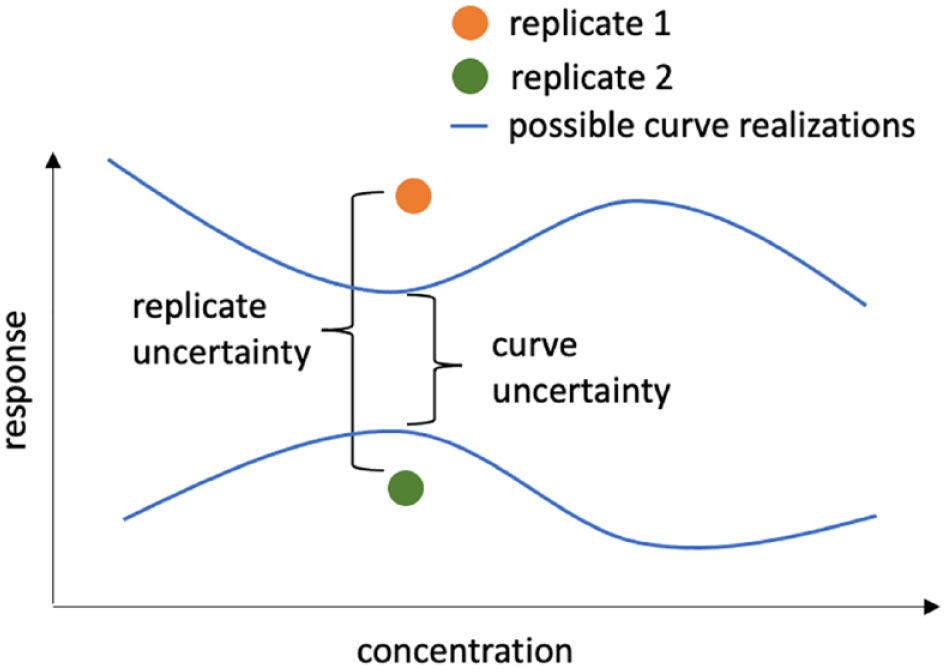
Sources of variation: curve uncertainty and replicate-to-replicate uncertainty.

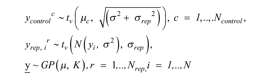
Variability in replicates for the same concentration y_{rep, i}^r, r = 1, . . ., N_rep, is modeled with a Student t distribution with degrees of freedom v, centered on the mean response and replicate-to-replicate scale σ _rep : y_{rep, i}^r ∼ t_v (y_i, σ_rep), where r = 1, . . ., N_rep. In vector notation this becomes

$$y_{rep}\sim t_v\left(y,{\sigma }_{rep}\right),$$

Here v is a parameter that is inferred from the data. The Student t distribution has heavier tails than the normal distribution and hence allows for more extreme observations. This choice makes the model less sensitive to outliers. The higher the estimate of v, the closer is the distribution to normal. Hence, the estimates of this parameter can diagnose the presence or absence of outliers in the data. To summarize, treatment data are distributed as

$$y_{rep}~t_v(N(\underset{\_}{y},{\sigma }^{2}I),{\sigma }_{rep}).$$

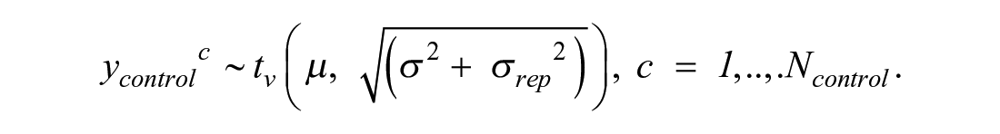
It would be hard to derive the analytical form of this distribution. However, to fit a Bayesian model, the analytical form of the distribution is also not needed. What we can notice is that the total variation of the replicates approximately equals σ² + σ_rep². Data for controls y_control^c, where c = 1, . . ., N_control, have mean µ and the same two sources of variation: curve uncertainty and replicate-to-replicate uncertainty. That is why, to match the amount of modeled uncertainty in the treatments, heuristically, the likelihood for controls is derived as

$$y_{control}{}^c\sim t_v\left(\mu ,\sqrt{\left({\sigma }^2+{\sigma }_{rep}{}^2\right)}\right),c=1,..,.N_{control}.$$

Distributions for y_rep and y_control define the likelihood of the model. The computational graph, summarizing this logic, is presented in Supplemental Figure S2 .

Changepoint Gaussian Processes

The trend y as the dependence of the outcome variable (protein degradation) on the concentration is modeled using a GP with a changepoint kernel. A composite GP kernel has been proposed in the context of dose–response curve fitting in Hatherell et al. ⁹ The proposed covariance structure is a special case of a changepoint GP. Here we present a more general framework of the changepoint kernel modeling and explain how Hatherell et al ⁹ fits into it.

A GP defines a probability distribution over functions; that is, each sample from a GP is an entire function, indexed by a set of coordinates (concentrations). Evaluated at a set of given concentrations, a GP f is uniquely specified by its mean vector µ and covariance matrix K and follows a multivariate normal distribution: f ~ N( µ , K ). Each element of the covariance matrix K_i,j is obtained as an evaluation of the covariance kernel—a function of two arguments k(., .) at a pair of points x_i and x_j. The kernel controls variance–covariance structure: its value at a set of two points k(x_i, x_j) quantifies the covariance of two random variables, f(x_i) and f(x_j). Kernel design is crucial for GP modeling since it describes the class of possible functions that can be captured: both the global shape and local properties, such as smoothness. ¹⁰ Most commonly used kernels, such as exponential η²exp(–d/ρ), squared exponential η²exp(–d²/ρ²), or Matern C_v,ρ(d), depend on the distance d = ||x_i – x_j|| between two points and hence are stationary. They are inappropriate for modeling CR curves and surfaces (e.g., drug–drug interaction), which might display different behavior across the observed concentrations. Kernels derived from exponential and squared exponential kernels would have smooth shapes, while Matern kernels, under certain values of ν, result in curves with more local fluctuations and less smoothness. The length scale ρ, common for many kernels, governs the flexibility of the curves. Smaller length scales induce correlations between points at smaller distances and hence more oscillatory behavior; such behavior, when exaggerated, can lead to overfitting. Too large length scales, on the other hand, make curve fits too inflexible and may lead to underfitting the data. The amplitude η, frequently applied to kernels as a constant multiplier, controls the expected variation in the output. The amplitude controls how strong the functions fluctuate and the length scale controls how rapidly they fluctuate. The dependence of the standard kernels on their parameters can be visually inspected in Görtler et al. ¹¹ The choice of priors of the GP parameters plays a big role in their identifiability.

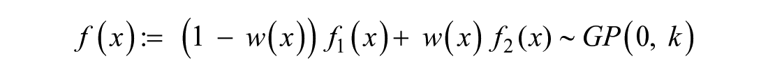
Covariance functions can be scaled, multiplied, summed with each other, and further modified to achieve a desired effect. For instance, if it is known that a curve behaves differently before and after concentration θ, a changepoint kernel can be used to provide a reasonable model. If the curve before θ can be described by

$$f_1(x)\sim GP\left(0,k_1\right),$$

and the curve after θ can be described by

$$f_2(x)\sim GP\left(0,k_2\right),$$

then the desired global GP can be constructed as a weighted average of the two local models,

$$f\left(x\right):=\left(1-w\left(x\right)\right)f_1\left(x\right)+w\left(x\right)f_2(x)\sim GP\left(0,k\right)$$

and its kernel function can be composed as

$$\begin{array}{l}k\left(x,x’\right)=\left(1-w_{\theta }\left(x\right)\right)k_1(x,x’)\left(1-w_{\theta }\left(x’\right)\right)\\ +w_{\theta }\left(x\right)k_2\left(x,x’\right)w_{\theta }\left(x’\right),\end{array}$$

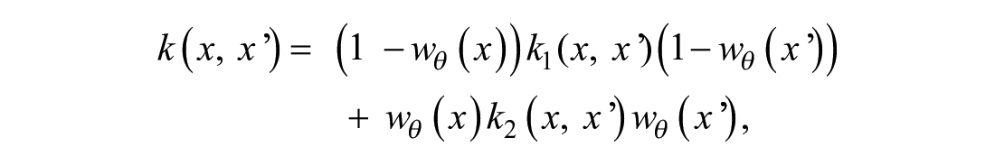
where w_θ(x) is a function with values between 0 and 1. The farther away is x from θ to the left, the closer is w_θ(x) to 0 (hence, k₁ will dominate in that region). The farther away is x from θ to the right, the closer is w_θ(x) to 1, and hence k₂ will dominate there. The standard choice of the weighting function is the sigmoidal w₀(x) = σ(x), providing a smooth transition from f₁ to f₂, centered around 0. However, the weighting function can be modified to shift the transition point from 0 to θ, w₀(x) = σ(x) → w_θ(x) = σ(x − θ), or make the transition more rapid, w_θ(x) → w_θ,g(x) = σ(g*(x – θ)) (g > 1), or slower (g < 1). If parameter g is a very large number, the transition function can be substituted with a step function s_θ(x) = 0 if x < θ and s_θ(x) = 1 otherwise. In practice, if one opts to use the step function as a weight w_θ(x), it is easier to formulate the changepoint kernel via an if–else statement. In our model formulation, g is a parameter and is estimated from data. The dependence of GPs with standard kernels (exponential, squared exponential, Matern, linear) on the values of their parameters is well understood. The novelty of the proposed kernel is in parameter g. A qualitative change of behavior of a curve, depending on the value of g, is presented in Supplemental Figure S3 . The figure shows how the values of g affect the shape of possible curves under such a kernel.

In the context of CR curve fitting, the data can be represented as a set of pairs (x_i, y _i ), where i = 1, . . ., N. Here x = x_i is the value of the unique input coordinate (concentration), y = y _i is the corresponding mean response, and N is the number of unique concentrations ( Fig. 2 ). For PROTACs, it is assumed that the expected response is constant at low concentrations up to a threshold concentration θ (the concentration threshold at which a chemical induces an effect, i.e., PoD). A linear kernel with no slope is appropriate to model such behavior (k₁ = 0) of the model to the left from θ. For concentrations above θ, the expected response is assumed to vary smoothly as a function of concentration, and it can either grow or decline. Hence, exponential or squared exponential kernels would make a reasonable choice for concentrations above θ. The kernel k₂ = η²(x_i – θ)²(x_j – θ)²exp(–(x_i – x_j)²/ρ²), defining the function to the right side of the threshold, is a product of the Gaussian and squared linear kernels. The Gaussian kernel η²exp(–(x_i – x_j)²/ρ²) provides smoothness, and a squared linear kernel (x_i − θ)²(x_j − θ)² allows the range of plausible values to increase together with the distance from the PoD θ.

Figure 2.

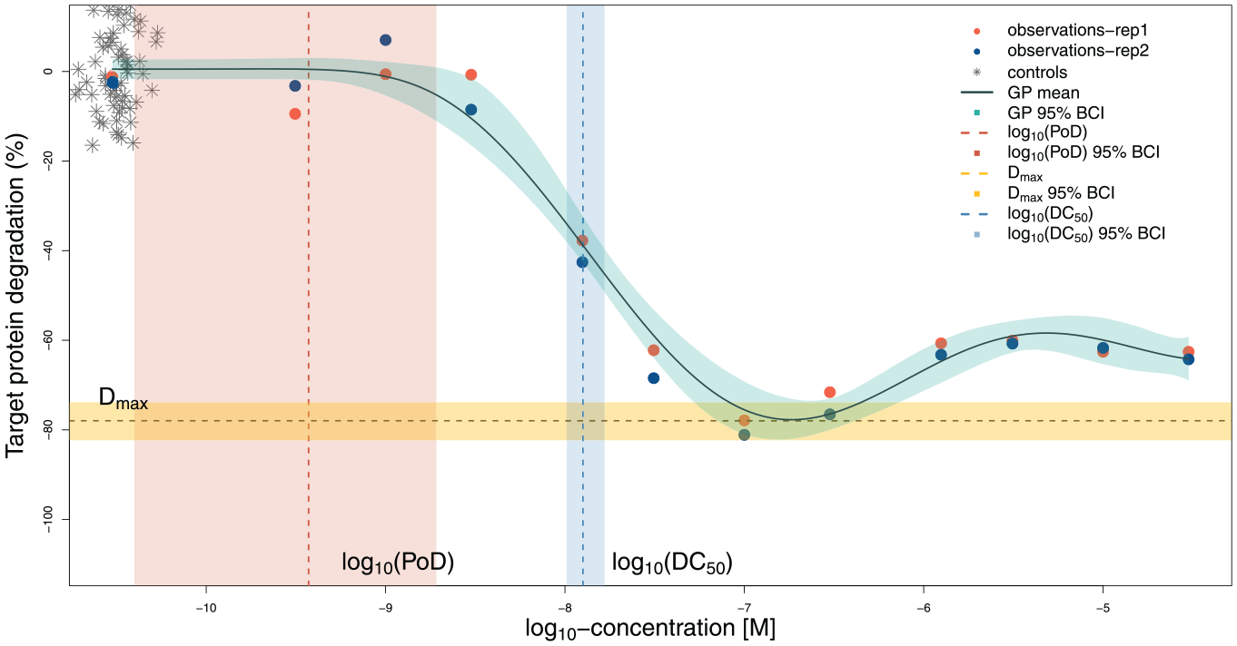
Prediction for one compound. The predicted curve, calculated estimates, and uncertainty intervals are shown. The PoD is estimated less precisely compared with the DC₅₀ and D_max. Controls are graphically overlaid at the lowest available concentration for treatments.

As the weighting function, we use w_θ,g(x) = σ(g*(x − θ)), where parameter g is inferred from data. Note that the kernel used in Hatherell et al. ⁹ is the special case of the above-described kernel, as the weighting function chosen there equals s_θ(x). By allowing g to be a parameter of the model, we allow more flexibility in the curve shapes.

GP Predictions

Only evaluations of the GP at measured concentrations x_i = x_obs,i are used for inference, but we are interested in finding continuous curves. To calculate curve trajectories, we define a grid of points (concentrations) at which we want to make predictions and calculate the values of f at the selected locations x_pred,i, where i = 1, . . ., N_pred. Jointly, observed and unobserved values are distributed as a multivariate normal:

$$\left(\begin{array}{c}{f}_{obs}\\ f_{pred}\end{array}\right)~N(\left(\begin{array}{c}{\mu }_{obs}\\ {\mu }_{pred}\end{array}\right),\left(\begin{array}{cc}{K}_{obs}& K_{obs,pred}\\ K_{obs,pred}& K_{pred}\end{array}\right)).$$

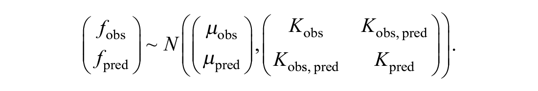
Due to the properties of the multivariate normal distribution, the distribution for the unobserved values given the observed values is given by N(m, Σ), with m = µ_pred + (K_obs,pred)^T*(K_obs)⁻¹*(f_obs − µ_obs) and Σ = K_pred − (K_obs,pred)^T*(K_obs)⁻¹*K_obs,pred. Here µ_pred = µ*[1, . . ., 1]^T is a constant vector, K_obs is the covariance matrix evaluated at observed locations, K_pred is the covariance matrix evaluated at locations for predictions, and K_obs,pred is the covariance matrix evaluated at the pairs of observed and prediction locations.

Priors for Model Parameters

Full Bayesian model formulation requires specification of prior distributions for parameters µ, σ, σ_rep, η, ρ, and θ. Baseline response µ is assigned the weakly informative prior µ ∼ N(0, 0.1). Scale σ, governing the concentration-to-concentration variation, is assigned the inverse gamma prior σ ∼ InverseGamma(1,2), implying a mode of 1. Scale σ_rep, governing the replicate-to-replicate variation, is assigned the inverse gamma prior σ_rep ∼ InverseGamma(1,0.1), implying a mode of 0.05. In this way, we express our belief that replicate-to-replicate variation for the same concentration is smaller than the deviation of measurements from the mean curve. The length scale, ρ, should not be smaller than the minimal distance between concentrations (about 0.5 on the log₁₀ concentration scale), and not larger than the range of concentrations (about 6 on the log₁₀ concentration scale). We use a gamma prior ρ ∼ Gamma(50,20) which does respect the constraints and has a mode of approximately 2.5. This implies that for log₁₀ concentrations between –10.5 and –4.5, correlations are nonnegligible at distances of about 40% of the total length of the concentration interval. For the amplitude η, we use a normal prior, η ∼ N(1, 1), and for the threshold θ, a uniform distribution between the lowest and highest concentrations, θ ∼ U(x_min, x_max). For degrees of freedom of the Student t distribution v, we use Gamma(2, 0.1). This prior has been proposed in Juárez and Steel ¹² and is now widely adopted by the Stan community. With a mean of 20 and variance of 200, it provides room for a wide range of values for v. Our prior for g is Gamma(10, 1), which has a mean of 10 and a variance of 10, and hence specifies a plausible range of values as informed by Supplemental Figure S3 .

Different Baselines for Treatments and Controls

The data normalization procedure includes the transformation x → (x – <cr>), where x is the raw measured response and <cr> is the median value for controls. As the mean and median of controls may not coincide, the difference between them can be nonzero. That is why we keep the parameter µ in the model, even if we expect its estimates to be close to 0. In data sets, where a lot of measurements of controls and only few measurements for each treatment dose are available, it can happen that µ would represent the mean of controls stronger than the treatment. In cases when the observed treatment response at low concentrations is not close to the mean of the controls, using µ as a baseline (value at low concentrations) for treatments may bias the response curve in the low-concentration area. To avoid such an effect, modification of the model can be used, where the base level of the treatment is estimated by the parameter µ and the mean of controls is estimated by a different parameter, µ_c. In that case, the likelihood of the model takes the form

$$\begin{array}{l}{y}_{control}{}^c\sim t_v\left({\mu }_c,\sqrt{\left({\sigma }^2+{\sigma }_{rep}{}^2\right)}\right),c=1,..,.N_{control},\\ y_{rep,i}{}^r\sim t_v\left(N\left(y_i,{\sigma }^2\right),{\sigma }_{rep}\right),\\ \underset{\_}{\mathrm{y}}~GP\left(\mu ,K\right),r=1,..,N_{rep,}i=1,..,N\end{array}$$

Usually, there will not be many controls available, and the model with µ_c = µ would be more appropriate. If this is not the case, however, we suggest using the baseline for treatment different from that of the mean of controls. For this version of the model, we suggest keeping the prior for µ_c as a normal distribution with mean 0 and standard deviation 0.1, and to choose the prior for µ as a normal distribution with mean 0 and standard deviation 0.2.

Calculating Biologically Relevant Parameters and Ranks

In the process of Bayesian inference, we collect samples of the model parameters and the mean GP curve, which form the posterior distribution. If N_iter draws (i.e., Markov chain Monte Carlo [MCMC] samples) have been saved, each of the curves can be used to derive further statistics, such as biologically meaningful quantities: DC₅₀, D_max, or PoD. We perform the computations based on each drawn GP to create a sampling distribution of the quantities. These distributions reflect uncertainty of the estimates. A PoD is directly represented in the model by its parameter θ; D_max is calculated as the maximal amount of degradation, that is, the minimal value on the y axis, and DC₅₀ is calculated as the abscissa of the half-maximal degradation point. To find DC₅₀ numerically, we first compute its ordinate y_DC50 and then search for a point with the lowest x value on the predictive grid with the minimal difference between the GP and y_DC50.

For each saved MCMC iteration i in this process, we create a ranking of compounds based on the magnitude of DC₅₀. If (DC₅₀)ⁱ _j is an estimate obtained from iteration i, i ∈ (1, N_iter) for compound j, j ∈ (1, N_cpds) (here N_cpds is the total number of compounds), then for a fixed i, the N_cpds estimates can be sorted. The order of the sorting yields the ranking of compounds, and the final rank of a compound is its most frequent rank of this compound across all iterations. This procedure is graphically presented in Figure 3 . Fitting of the Bayesian model for each compound is taking place independently from other compounds. In the presence of a large number of compounds that need to be compared, this step can be parallelized and will not lead to increased computation time. Once all posterior samples have been collected, the sorting step is applied to each iteration i independently and, again, can be parallelized.

Figure 3.

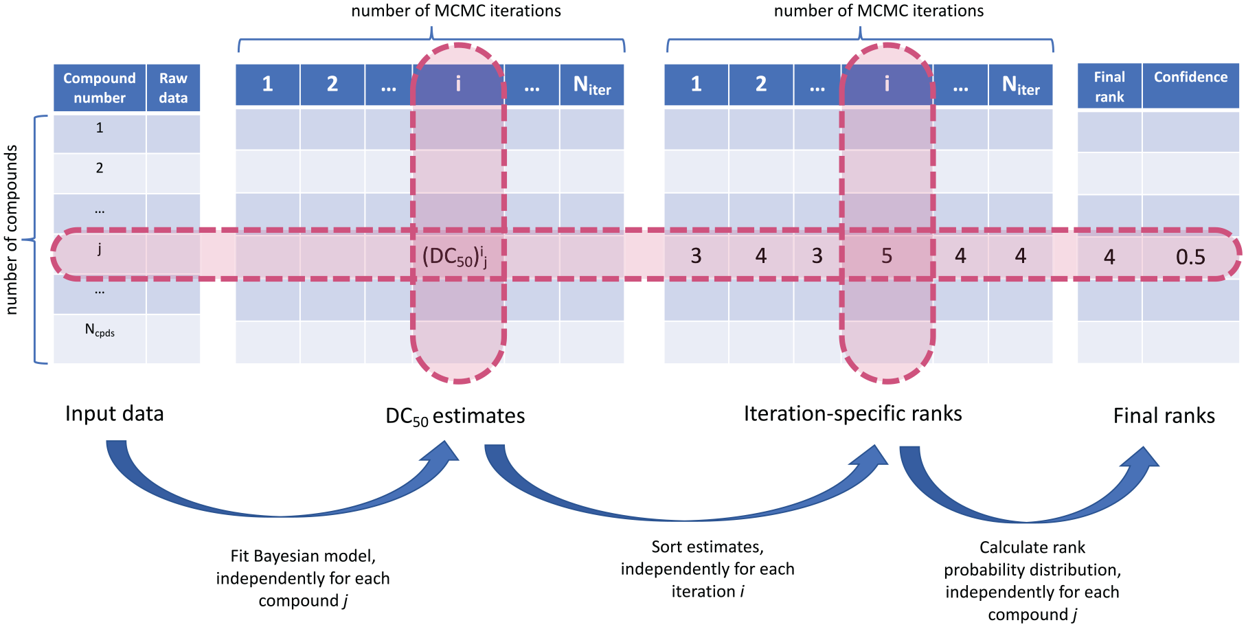
From raw data to compound ranks.

Software

The model was fit in Stan, ¹³ which uses a Hamiltonian Monte Carlo sampler. We used RStudio ¹⁴ to process the data and interface with Stan. The Bayesplot ¹⁵ library was used to visualize convergence statistics. We used four chains of 10,000 steps each to produce draws from the posterior. Convergence has been evaluated numerically using R-hat and effective sample size statistics. R-hat compares within-chain variation and between-chain variation, and effective sample size is an estimate of the number of independent draws from the posterior distribution. There are no strict thresholds for both statistics, but general guidance is that R-hat should be close to 1 and an effective sample size should not be too small as compared with the total number of samples. Visual inspection of posterior distributions of model parameters ( Suppl. Fig. S4 shows results for one compound) also demonstrated convergence as posterior distributions from different chains agree well. The mean elapsed CPU time (on a laptop with 2.3 GHz Intel Core i5 and 8 GB memory) for four chains was 9.23 s with a standard deviation of 1.22 s. Estimates of model parameters for one compound are presented in Supplemental Table S1 . Predictions were made on a regular grid of N_pred = 1000 points spaced between the minimal and maximal concentrations. Produced estimates of biologically relevant parameters are presented in Supplemental Table S2 . The code for fitting the data to one compound using the logistic function as a weight function, w_θ,g(x) = logit⁻¹(g*(x – θ)), is available on GitHub: https://github.com/elizavetasemenova/gp_concentration_response.

Results

First, we fit the model to one compound with 12 concentrations (the dosage currently used in practice) and two replicates and discuss the results in detail. Next, we analyze nine compounds with 18 concentrations. Data of the two experiments were available, and each experiment contained two replicates. In this way, the combined data set provides four replicates per concentration for each of the nine compounds. We demonstrate uncertainty in the produced ranking based on DC₅₀ and suggest extending this metric to also include D_max. Finally, we fit the alternative model with different baselines for treatments and controls to all nine compounds.

Example of One Compound

This data set contains 12 concentrations with two replicates per compound. Figure 2 shows the mean prediction, which closely follows the main trend in the data, and the quantile-based (95%) BCI ¹⁶ (shaded region around the curve). Despite the nonsigmoidal shape, the model accurately detects the lowest part of the curve, which indicates the maximal effect (D_max). In addition, the model automatically estimates a sensible value for the DC₅₀—similar to where a person might draw a vertical line. The PoD is estimated with less precision but covers the range of concentrations where the curve is largely flat.

Uncertainty in Ranking of Compounds

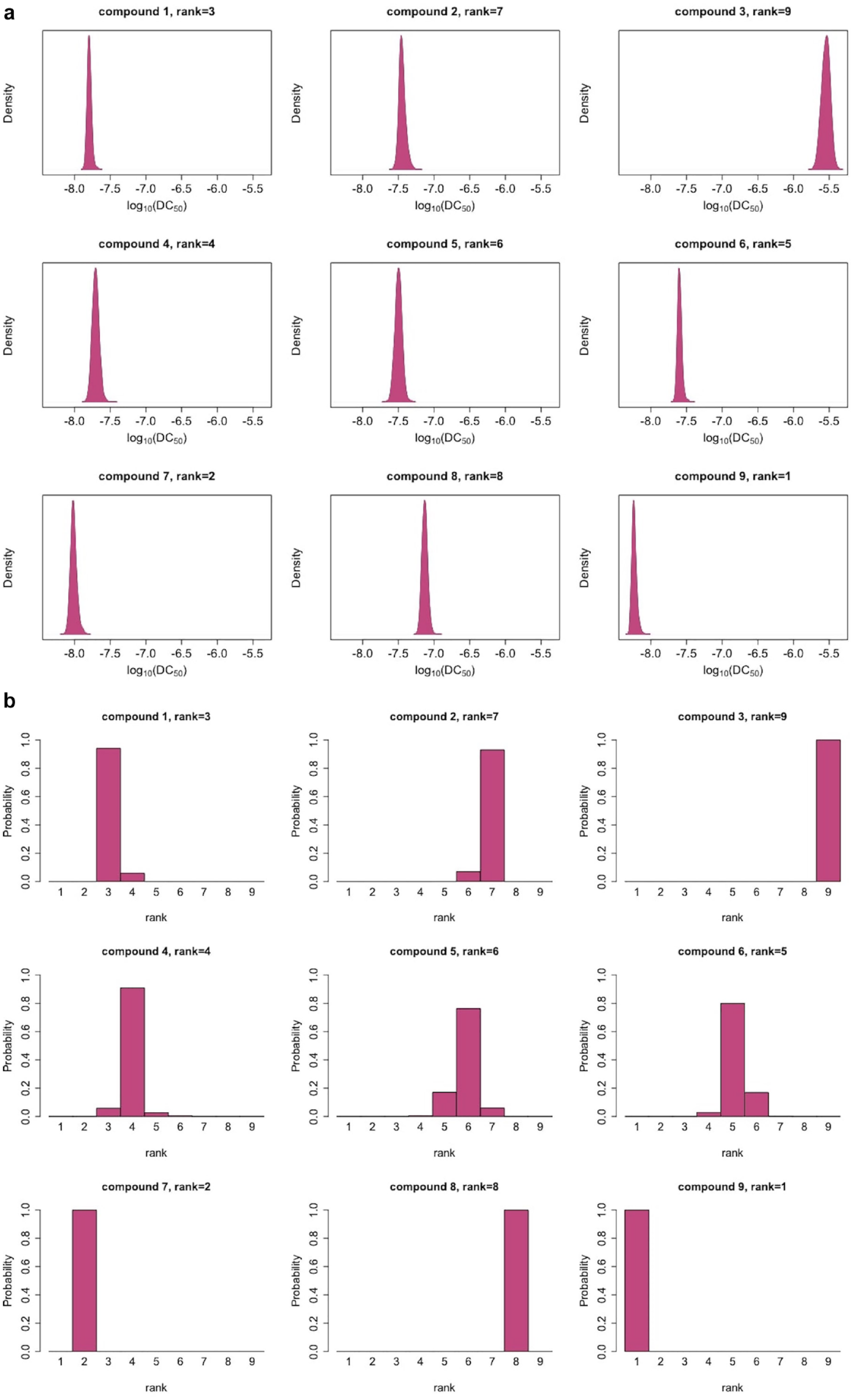
The data in Figure 4 are from two experiments at 18 concentrations and with two replicates per experiment. This is a very high resolution and would be rarely available in a screening process, and hence they yield tight uncertainty bounds for log₁₀(DC₅₀). However, even low uncertainty in the estimates translates into uncertainty of the rankings for many compounds. Figure 5a displays posterior distributions for the log₁₀(DC₅₀) values, and Figure 5b displays the resulting ranks and their uncertainty. Figure 4 shows that for most of the compounds the model provides sensible fits. Compounds 2 and 5 display a similar pattern: there is a discontinuity in the trend of the data. The fitted curve does not exactly fit the points at lower concentrations or points at about –8.2 concentrations (on the log₁₀ scale), but rather finds an average trend between the two extremes. While the model does not overfit, discontinuity in the data is reflected in the uncertainty of the curve estimates in the neighborhood of this concentration. Furthermore, the model behaves robustly with respect to the outlier of compound 2 (at log₁₀ concentration of 6). Compounds ranked as the best (ranks 1 and 2) and the worst (ranks 9 and 8) are very distinct, while uncertainty in the ranks is higher for the other compounds.

Figure 4.

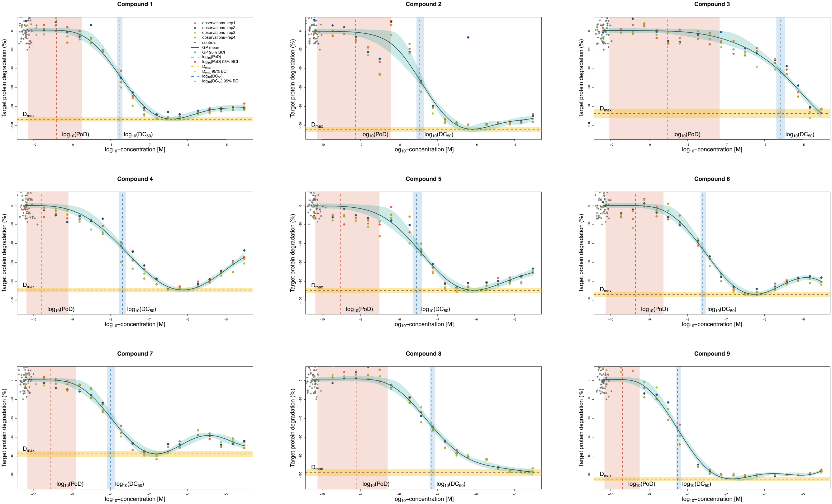
GP model fits of nine compounds, with four replicates each. The flexibility of the model allows it to fit a variety of CR relationships, and despite some nonsigmoidal shapes, the estimated DC₅₀ and D_max values correspond to what a person might draw by hand. Controls are graphically overlaid at the lowest available concentration for treatments.

Figure 5.

(a) Posterior draws of log₁₀(DC₅₀) values. (b) Resulting ranks of compounds together with their uncertainty.

Decisions made solely on DC₅₀ might overlook other important properties. Other estimated parameters of the model or the derived biologically meaningful quantities can be used for ranking. For instance, the maximal degradation D_max carries important information about a compound. There is a multitude of ways to choose a ranking measure. Here we present how the combination of DC₅₀ and D_max can be used. Figure 6 displays the estimates and BCIs for both parameters. Compounds in the bottom left quadrant are preferable. This agrees well with the ranking of compound 9—it has the lowest log₁₀(DC₅₀) and log₁₀(D_max); however, compound 7, confidently ranked second according to log₁₀(DC₅₀), shows less maximal degradation and potentially would be de-prioritized if more information was taken into account. We suggest using a weighted combination of log₁₀(DC₅₀) and log₁₀(D_max): D_comb $=\alpha {\stackrel{\sim }{DC}}_{50}+(1-\alpha )\stackrel{\sim }{D_{\max }}.$ Here ${\stackrel{\sim }{DC}}_{50}$ and $\stackrel{\sim }{D_{\max }}$ are log₁₀(DC₅₀) and log₁₀(D_max) rescaled to the [0, 1] range, and α ∈ [0, 1] is the weighting coefficient, which can be chosen by a scientist to give more preference to DC₅₀ (α close to 1), weight DC₅₀ and D_max equally (α = 1/2), or prioritize D_max (α close to 0). Using the weighted metric, we recalculate ranks of the nine compounds according to different values of α ( Table 1 ). We have performed the scaling by subtracting the minimal value of all samples and dividing by the difference between minimal and maximal values of all samples.

Figure 6.

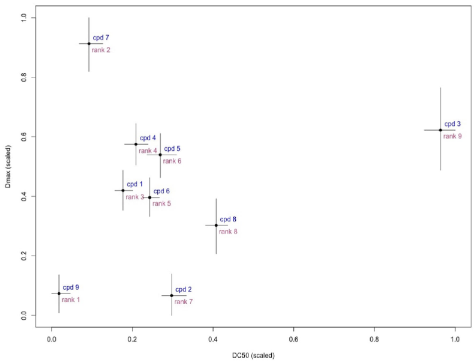
Two or more parameters can be used to rank compounds: compounds with low values of $\stackrel{\sim }{D{C}_{50}}$ (scaled log₁₀(DC₅₀)) and $\stackrel{\sim }{D_{\max }}$ (scaled D_max) are desirable as they indicate high potency and large effects. Compound 9 is distinguished as the best by these criteria. Error bars are 95% BCI.

Table 1.

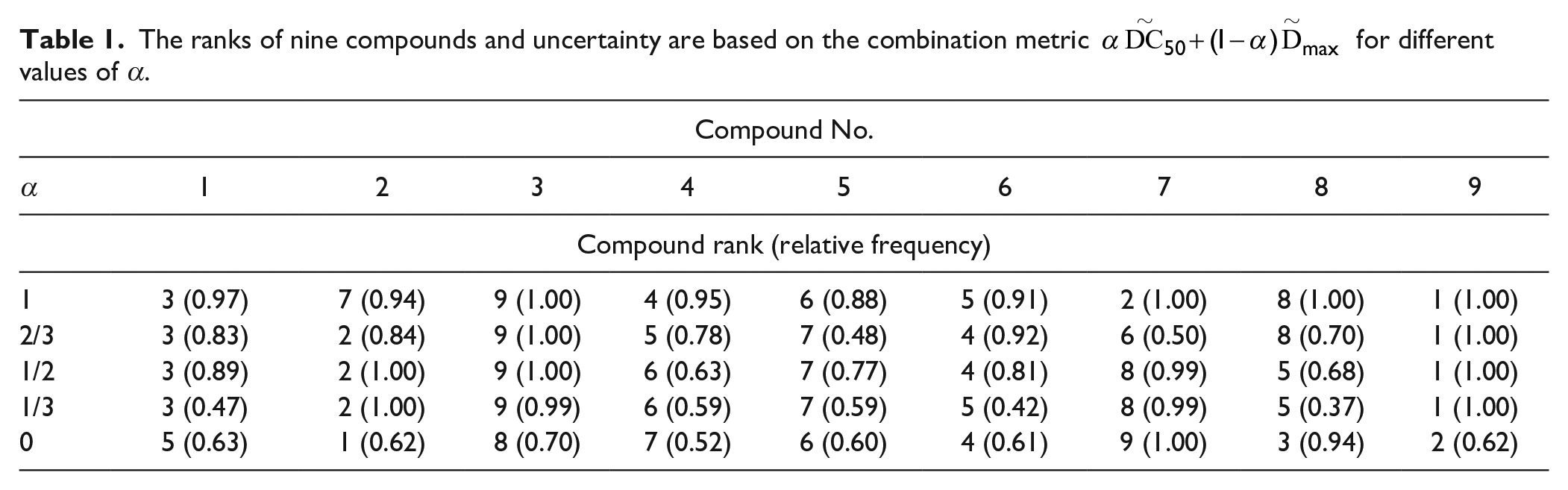
The ranks of nine compounds and uncertainty are based on the combination metric $\alpha \stackrel{\sim }{D{C}_{50}}+(1-\alpha )\stackrel{\sim }{D_{\max }}$ for different values of α.

Compound No.
α	1	2	3	4	5	6	7	8	9
Compound rank (relative frequency)
1	3 (0.97)	7 (0.94)	9 (1.00)	4 (0.95)	6 (0.88)	5 (0.91)	2 (1.00)	8 (1.00)	1 (1.00)
2/3	3 (0.83)	2 (0.84)	9 (1.00)	5 (0.78)	7 (0.48)	4 (0.92)	6 (0.50)	8 (0.70)	1 (1.00)
1/2	3 (0.89)	2 (1.00)	9 (1.00)	6 (0.63)	7 (0.77)	4 (0.81)	8 (0.99)	5 (0.68)	1 (1.00)
1/3	3 (0.47)	2 (1.00)	9 (0.99)	6 (0.59)	7 (0.59)	5 (0.42)	8 (0.99)	5 (0.37)	1 (1.00)
0	5 (0.63)	1 (0.62)	8 (0.70)	7 (0.52)	6 (0.60)	4 (0.61)	9 (1.00)	3 (0.94)	2 (0.62)

All nine compounds presented in Figure 4 are active compounds, that is, they respond to the increasing concentration in a significant way. We have tested our model on simulated “flat” data to verify that it would deal with inactive compounds appropriately. For this, we have simulated responses with a mean equal to the mean of controls and a standard deviation that equals 1.1 standard deviation of controls. Supplemental Figure S5 displays the fits of the Bayesian Hill model and the changepoint GP model to such data. Changepoint GP produces a nearly flat fit with D_max estimates close to the mean of the simulated data.

Results of the model with different baselines for treatments and controls are presented in Supplemental Figure S6 . Uncertainty in µ_c is higher than in the model with equal baselines due to both a wider prior for µ and less data available for its estimation.

Discussion

We have used a changepoint GP CR model, coupled with Bayesian inference of its parameters, to flexibly fit PROTAC CR curves. A Bayesian approach is advantageous for small amounts of data and can represent uncertainty of the parameters and derived estimates in the form of distributions. A GP model does not require strong assumptions on curve shapes, as parametric models do. The model is stable to outliers due to use of a Student distribution. The presence of outliers can be diagnosed using the estimates of the parameter v. Nonidentifiability is a frequent problem for GPs; often, only one of the length scale or amplitude parameters can be identified, while the other parameter needs to be fixed for the analysis. We have used an informative prior for length scale and have not encountered problems under the specified settings.

We have demonstrated how uncertainty in the estimates of DC₅₀ influences uncertainty in ranks and have proposed a single metric to capture both DC₅₀ and D_max. This metric involves a weighting parameter that allows a scientist to choose their decision-making approach and tackle ranking in a quantified manner. We have demonstrated that the ranks of the worst (rank = 9) and the best (rank = 1) compounds are fairly stable with respect to the varying weighting coefficient, while the ranks of less clear leaders (e.g., compounds 2 and 7) may change their ordering. Currently, decisions are mainly made based on DC₅₀, which corresponds to α = 1. The weighting can be extended to more parameters, for example, DC₅₀, D_max, and θ, if they all represent interest for screening; the combination metric would weight all three estimates ${\alpha }_1{\stackrel{\sim }{DC}}_{50}+{\alpha }_2\stackrel{\sim }{D_{\max }}+{\alpha }_3\stackrel{\sim }{\theta }$ with α₁ + α₂ + α₃ = 1, α_k ∈ (0,1).

For parametric models, such as a sigmoidal or double sigmoidal, the area under the curve (AUC) can be used as a single measure of a compound’s potency. This approach, however, is less applicable to GP fits since such curves might experience local fluctuations. These fluctuations would have little influence on the estimates of parameters such as DC₅₀, but cumulatively might contribute nonnegligible amounts of AUC, leading to erroneous conclusions. A potential solution could be computing AUC for GPs only in the domain between the minimal concentration and the first concentration where the maximal effect D_max is achieved. In our example, we have mapped DC₅₀ and D_max by scaling. Alternative approaches can be used, such as desirability functions. ¹⁷

The proposed model has been used internally to answer a set of experimental design questions, such as “Is it better to have more concentrations or more replicates?” A series of comparisons has been done between four, three, two, and one replicate for 18 concentrations, and between different numbers of concentrations (9 and 18) for the same number of replicates. An example of 18 and 9 concentrations (two replicates each), for the same compound as shown in Figure 2 , is shown in Supplemental Figure S2 . The plot shows slightly more uncertainty in the model fit produced using nine concentrations, while the general shape of the fit and DC₅₀ estimate remain close. Model fits based on four, three, and two replicates for the same compound are presented in Supplemental Figure S8 . Both the curve shapes and amount of uncertainty are similar for all three fits. Our conclusion from this exercise, evaluating the trade-off between number of replicates and number of concentrations, was that more concentrations is preferred to more replicates, and that 12 concentrations with one replicate is sufficient to produce a robust ranking.

The changepoint kernel, used in this work, fits a flat curve to the data to the left side of the PoD and does not use the mechanistic understanding of the model otherwise. As a result of that, some GP fits might display minor local fluctuations at higher concentrations, which a parametric model would not do. Nevertheless, these fluctuations would not have a major impact on the estimates of the estimated parameters and ranking. If it is important to capture more mechanics in the curve-fitting step, it can be done by further expansion of the changepoint kernel. For instance, in the case of PROTACs, one would expect the curve to flatten out after the hook. The changepoint kernel, in this case, would have three GP components (flat linear, smooth, and flat linear) and two inflexion points, θ₁ and θ₂. Derivations of the kernel in this case are provided in the Supplement. Another solution to the local fluctuations at high concentrations could be provided by a concentration-dependent length scale, such as ρ²(1 + (x_i −θ)²)(1 + (x_j − θ)²). ¹⁸

GP models are computationally more involved than parametric models. Running MCMC samplers might take longer than applying traditional (frequentist) parametric methods. As a result, incorporating Bayesian GP models into workflows might be less straightforward. However, as computational tools evolve, this limitation will be gradually diminished. Furthermore, frequentist optimization techniques have their own difficulties, such as subjective choice of initial values, and might have convergence issues.

The most time-consuming steps in the compound-ranking process are fitting of the Bayesian model and predicting the amount of degradation at unobserved concentrations. As the model can be fit to each of the compounds independently, it takes the same amount of time to fit all compounds as it takes to fit one compound. Fitting of one compound on our machine takes, on average, 9 s (with a standard deviation of 1.2 s between four chains). As the model is fit to the data for each compound independently, the process can be parallelized without additional time cost. The sorting procedure that provides the ranks is not specific to Bayesian methods and would be needed in a standard ranking procedure as well. The overall computation time is a trade-off with the number of iterations for Bayesian model fitting and the number of concentrations at which the response needs to be predicted.

Among the nine presented compounds, one of them (compound 3) could not have reached its D_max. The estimates produced by the changepoint GP model reflect the uncertainty in a wider BCI as compared with other compounds. The fit of compound 3 does not have an asymptote at higher concentrations, as values at these concentrations keep declining monotonically. This is an issue of the range of observed concentrations, and not of the model. The width of the uncertainty interval for D_max here is wider than for other presented compounds fitted by the changepoint GP model. For comparison, we have also produced Bayesian fits of the four-parameter (4PL) model to the data, accounting for the same source variation as described above, and the mean curve modeled as y = d + (a – d)/(1 + exp(–b(x – c))), where d denotes the amount of degradation at 0 concentration; a denotes D_max,c, which stands for log₁₀(DC₅₀); x is log₁₀ dose; and b is the Hill slope. More details and produced fits for all nine compounds are available in Supplemental Figure S9 . For compound 3, the BCI of D_max produced by the 4PL model is (–90.11, –85.93) and has the width 4.18; the BCI produced by the changepoint GP model is (–91.66, –82.49) and has the width 9.17; non-Bayesian fit of the 4PL model (obtained using the drc R-package ¹⁹ ) produces a CI of (–309.2, –67.86) of width 242. While the width of the BCI by the changepoint model might be narrower than intuitively expected, the CI by the frequentist model is too wide: its upper limit of approximately –67 is much higher than the observed degradation at high concentrations (below –80). Additional quantities can be calculated to resolve this issue and verify whether D_max has been attained. The derivative of the function approaching D_max should be nearing 0, and hence the absolute value of the slope of the curve should be small. The magnitude of this derivative can be incorporated into the estimation of uncertainty of D_max. In this work, we have used data preprocessed by GeneData via the normalization step. The shift x – <cr> moves raw data x up or down by the mean of the controls to make all curves start at the value of approximately 0. The distribution of neutral controls is tight, and its mean and median are not far from each other. The estimates of parameter µ confirm that this is a very small number (see Suppl. Table S1 ) and its credible interval includes 0. The entire transformation (x – <cr>)/(<sr> – <cr>) ensures that all data points lie approximately between 0 and –100. Hence, normalization affects curve-to-curve range and enables comparability of curves and produced estimates. For the case when treatment response at low concentrations is not close to the median of controls, we have suggested an alternative model with different baselines of treatments and controls. For compounds with lower base level µ than in a model with equal baselines, for example, compounds 2 and 5, POD has shifted to the right; on the contrary, the POD of compounds with higher µ, for example, compounds 8 and 9, POD has shifted to the left.

Unlike parametric models, it is more difficult to link GPs to a mechanistic understanding. And sometimes models might display minor local fluctuations, which a parametric model would not have. Nevertheless, these fluctuations would not have a major impact on the parameter estimates and ranking. We believe that this approach has a lot of potential and can be used by pharmaceutical companies by taking steps toward its automation. If the assumption about possible curve shapes holds, important choices to make are the priors and the degrees of freedom in the Student t distribution.

Supplemental Material

sj-pdf-1-jbx-10.1177_24725552211028142 – Supplemental material for Flexible Fitting of PROTAC Concentration–Response Curves with Changepoint Gaussian Processes

Supplemental material, sj-pdf-1-jbx-10.1177_24725552211028142 for Flexible Fitting of PROTAC Concentration–Response Curves with Changepoint Gaussian Processes by Elizaveta Semenova, Maria Luisa Guerriero, Bairu Zhang, Andreas Hock, Philip Hopcroft, Ganesh Kadamur, Avid M. Afzal and Stanley E. Lazic in SLAS Discovery